Laser stimulated deexcitation of Rydberg antihydrogen atoms Preprint: APS/123-QED
Abstract
Antihydrogen atoms are routinely formed at CERN in a broad range of Rydberg states. Ground-state anti-atoms, those useful for precision measurements, are eventually produced through spontaneous decay. However given the long lifetime of Rydberg states the number of ground-state antihydrogen atoms usable is small, in particular for experiments relying on the production of a beam of antihydrogen atoms. Therefore, it is of high interest to efficiently stimulate the decay in order to retain a higher fraction of ground-state atoms for measurements. We propose a method that optimally mixes the high angular momentum states with low ones enabling to stimulate, using a broadband frequency laser, the deexcitation toward low-lying states, which then spontaneously decay to ground-state. We evaluated the method in realistic antihydrogen experimental conditions. For instance, starting with an initial distribution of atoms within the manifolds, as formed through charge exchange mechanism, we show that more than 80% of antihydrogen atoms will be deexcited to the ground-state within 100 ns using a laser producing 2 J at 828 nm.
I Introduction
Recent breakthroughs were achieved in spectroscopy measurements on antihydrogen atoms which led to stringent tests of the CPT symmetry, the combination of the charge conjugation, parity and time reversal symmetries ALP182; ahmadi2016improved; 2017Natur.548…66A. These measurements were all performed on magnetically trapped ground-state antihydrogen atoms which is currently the only method succeeding in accumulating enough ground-state atoms for measurements. Indeed, antihydrogen atoms formed at CERN, using three-body recombination or charge exchange processes, are produced in a broad range of Rydberg states including all possible angular momentum states ROB08; RAD14. The highly excited atoms must first decay before a precision measurement can be performed. Trapped atoms can be held on for hours ALP172 so that the produced Rydberg atoms have ample time to decay. In beam experiments however, the spontaneous lifetimes of the Rydberg states are hindering a fast enough ground-state population MAL18. Neglecting first the effect of external fields on the spontaneous lifetime of a () state (where ), the lifetime can be approximated by 2003PhRvA..68c0502F:
This result is also confirmed in a magnetic field environment. For instance Ref. Topccu2006 shows that within the 1-5 Tesla field present in antihydrogen experiments and for the three-body recombination formation mechanism, only 10% of the population with reach the ground-state in 100 s. A much longer time (2 ms) is required to have 50% of the population reaching the ground-state due to the large proportion of states with high angular momentum. Because antihydrogen atoms are typically formed with velocities of (corresponding to the mean velocity of a Maxwell-Boltzmann distribution at 50 K), if they are not trapped, they will hit the walls of the formation apparatus and annihilate long before any spontaneous deexcitation to ground-state can occur.
It is therefore of high interest to enhance the decay. It has been suggested that coupling or mixing high angular momentum states with low ones may accelerate the decay 2011JPhB…44n5003H. The main idea of the present article is to mix all angular momenta using an electric field added to the already present 1-5 Tesla magnetic field of the antihydrogen experiments and use a laser to stimulate the decay from high-lying states to a deep-lying one with a short spontaneous lifetime. The principle of the proposed scheme is sketched in Fig. 1.

We first estimate the feasibility of the method using a simple model assuming a fully mixed system and confirm that the laser power required is compatible with existing lasers and that photoionization can be drastically reduced by choosing a low enough manifold. We then discuss the validity of the first order treatment in the electric and magnetic fields and show that an optimal configuration of fields can lead to a large mixing of the states. Finally using this optimal configuration of fields we study in more details the effect of the laser power and polarization.
II General considerations assuming fully mixed states
For the sake of simplicity we focus here on antihydrogen formed in a pulsed charge exchange process 2016PhRvA..94b2714K.
The other formation mechanism used by the antihydrogen experiments is based on “continuous” three-body recombination of positrons and antiprotons (lasting as long as the antiproton and positron clouds can be kept in interaction, typically several hundreds of milli-seconds) producing typically
ROB08; RAD14.
This “continuous” production mode will be the focus of another publication where we will show that THz light can be efficiently used to stimulate the decay COM18. Consequently, we assume an initial distribution of states with full degeneracy in and as planned to be produced in the AEgIS experiment 2016PhRvA..94b2714K.
Before studying in detail the mixing mechanism in §III let’s first assume the presence of an electric and magnetic field resulting in a perfect state mixing. We can already see that such hypothesis is likely to be valid by estimating the first order Zeeman and Stark effects (see §III.1) which indicate that for (with ) an electric field of the order of 100 V/cm is sufficient to produce a Stark effect bigger than the spacing between Zeeman sublevels leading to a strong mixing of the (Zeeman) states as expected.
The assumption of perfect state mixing will allow us to evaluate the laser properties needed to stimulate the decay. The first obvious requirement is that the laser has to be broadband: in order to cover all Rydberg states we need a laser linewidth on the order of 2 5000 GHz. Note, that with such bandwidth we can also cover .
II.1 Fully mixed states hypothesis
We assume a fully mixed initial state that is coupled to the lower manifold thanks to a (spectrally Lorentzian) laser of FWHM and of central wavelength . We first consider an isotropic polarization of the light. We can then calculate the stimulated emission and photoionization rates for a given laser intensity .
II.1.1 Stimulated emission and photoionization rates
The stimulated emission rate under an unpolarized light is given by the sum over all polarizations and over all final states : , with where is the radial overlap given in Eq. (9) of the appendix.
Similarly, using the extra photon energy above the ionization threshold given by , we find the photoionization cross section: , where is the photoionization cross section from to given by: . is the radial overlap given by Eqs. (13) and (14) in the appendix.
Finally, the photoionization rate is and, because the cross section (and also the value) does not vary significantly over the laser spectral bandwidth we have
II.1.2 Saturation energy required
In order to have an efficient transfer toward the ground-state we need to transfer the population in a time scale compatible with the laser pulse and the spontaneous emission lifetime of the levels.
We study two extreme cases. The first one assumes a short nanosecond (10 ns) laser pulse for which we calculate the saturated intensity such that the stimulated decay rate is . In the second case we simply require a pulse duration comparable to the spontaneous emission lifetime of the manifold and calculate the saturated intensity such that the stimulated decay rate is 1/. Obviously , but we find useful to indicate both values.
For this first study we choose that is
the
average decay rate (over all levels) of the manifold.
It is calculated using where is the spontaneous emission rate from an state toward all sub-levels ( is the transition energy).
| (nm) | (ns) | (mJ) | (10 ns) (mJ) | |||
| 30 | 10 | 10 250 | 1908 | 0.0043 | 0.82 | 0.78 |
| 20 | 10 | 12 150 | 1908 | 0.00029 | 0.056 | 0.78 |
| 30 | 5 | 2343 | 86.5 | 4.4 | 38.5 | 6.0 |
| 20 | 5 | 2430 | 86.5 | 0.51 | 4.4 | 6.0 |
| 30 | 4 | 1484 | 33 | 37 | 124 | 11.4 |
| 20 | 4 | 1518.8 | 33 | 4.5 | 14.9 | 11.4 |
| 30 | 3 | 828.4 | 10 | 548 | 548 | 26.3 |
| 20 | 3 | 839.0 | 10 | 68.7 | 68.7 | 26.3 |
| 30 | 2 | 366.1 | 2.1 | 20 708 | 4405 | 84.6 |
| 20 | 2 | 368.2 | 2.1 | 2670 | 568 | 84.6 |
The results on the required saturation energy, assuming a laser waist of 1 mm (similar to the typical antiproton plasma size, see e.g. AGH18), as well as the ratio , are shown in table 1 and in Fig. 2.
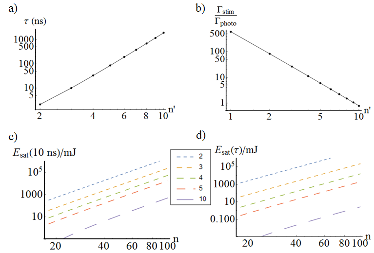
We first see that the competing effect of the photoionization toward the continuum is relatively weak especially for low values. This is due to the fact that the photoionization cross section drops quickly for high angular momentum states which are the most numerous states and that lower implies shorter laser wavelength that also reduces the photoionization effect.
Obviously, the power required to deexcite increases with decreasing due to the scaling of the dipole matrix element and to the fact that fewer angular momenta () exist and can be coupled to the initial ones.
Based on these results we see that several laser choices are possible.
Toward , power in the Watt range is enough and some CO2 lasers exist that can even allow a continuous deexcitation scheme for high values wan1985study; gupta1990various.
But lower are better to minimize photoionization. Deexcitation toward seems feasible using a laser similar to the one used by AEgIS to excite positronium (a bound state of electron and positron) to Rydberg states AGH16. However the use of a nanosecond laser with a pulse much shorter than the spontaneous emission lifetime of the states will limit the transfer by equalizing population between upper and lower levels.
Therefore, targeting a lower state, like , will improve the deexcitation efficiency. Furthermore intense lasers that have a long pulse duration (100 ns) in the Joule range exist at this wavelength. This is the case for the alexandrite WAL85 which can reach through heating of the medium KUP90.
III Mixing in electric and magnetic fields
For the next study we therefore restrict ourselves to , but most of the results will be valid for any other case.
Here we study in more detail the mixing produced by an electric and a magnetic field. We neglect the spins because Stark and Zeeman effects in the Rydberg manifold usually dominate the fine or hyperfine effects.
III.1 First order Stark and Zeeman effects
Considering a given manifold, we have the following Hamiltonian:
| (1) |
Atomic units will be assumed in this section.
Here, we use perturbation theory in the field values (not to be confused with the standard state perturbation theory). To the first order in the fields’ values we simply have to deal with the perturbation . We can indeed neglect the second order term since it is of the order of in atomic units (so for and ) solovev1983second; PhysRevA.57.1149; braun1993discrete. Thus, the second order becomes comparable to the first order (that is of the order of ) for and for a 1-5 Tesla field. Therefore, in our configuration, the first order should be accurate enough to extract the required fields values and laser energy.
The Hamiltonian (1) has been studied by Pauli who showed that, for a given manifold, , where is the Runge-Lenz vector. So in this manifold we can define new angular momenta and that commute and verify . We will use the basis where the eigenvalues (on a given axis) take the values . We define and such that . That is trivial to diagonalize using the basis. This notation indicates that is the projection of on the axis. So the first order perturbation theory gives
| (2) |
where .
For a pure electric field we restore the pure Stark effect with a clear relation to the parabolic basis linked to eigenvalues: and demkov1970energy; solovev1983second.
In a pure magnetic field we restore the standard Zeeman shift where because .
Using and the standard sum of the two angular momenta leads to or where the subscript B indicates that the quantization axis is along .
If we define and as the angles between the magnetic field axis and the vectors and respectively by the use of the Wigner rotation matrix, we have demkov1970energy (Eq. 1.4 (35) of varshalovich1987quantum) :
So by combining the equations (we use real Clesch-Gordan and real Wigner (small) -matrix ) we get:
| (3) | |||||
| (4) |
where we have written to stress that the angles depend on and not only on the fields’ values. Similarly . And we have the closure expression .
We can note that using such a () formalism the states will always be given in a parabolic basis not in a spherical basis, so even in a pure magnetic field the eigenstates will not correspond to the ones: is mixed in the basis.
III.2 Laser transitions under combined electric and magnetic fields
In order to choose the electric field which most optimally mixes the states, we need to calculate all transitions dipole moments from a given toward each states of the manifold. The Zeeman and Stark effect being small for we use the basis. So the stimulated emission rate, for a polarization, from an state toward all the manifolds is given by :
that can be calculated using Eq. (8) of the appendix and (4) in III.1.
The laser driven evolution of these states may be quite complex with levels coupled to ones (and to the continuum). Rate equations is sufficient to treat the problem assuming that the broadband laser used to stimulate the deexcitation is incoherent (which is likely to be the case). Furthermore, because we have chosen the with a fast spontaneous emission lifetime, the population of the levels will be small and the re-excitation process from to the manifold will not be severe. We can therefore consider that the levels are isolated from each other and thus simplify the picture to a 4 levels rate equation system as shown in Fig. 1:
| (5) | |||||
Cumbersome analytical solution exists for , the transfer of a given state to ground-state, and we use them throughout this article. However in this section we can simplify the solution because, as seen in table 1 and Fig. 2) we can safely neglect the photoionisation. We can also assume an instantaneous spontaneous emission from to ground-state if the laser pulse duration is much longer than the spontaneous emission lifetime of 10 ns (which can be considered the case for a e.g. 100 ns-long laser pulse as is the case for the alexandrite for example). In this case, the model becomes a simple two levels model, and the transfer of a given state to ground-state, after the application of the laser of polarization and of duration , is given by

Assuming an equidistribution of the
initial states we sum over these states to get
the total amount of atoms reaching ground-state. Results
are given in Fig. 3 as a function of and for different laser polarizations. We have used, in cartesian coordinates with , the result
.
The calculation has been performed for with a laser energy of 150 mJ and a pulse of 100 ns (but similar results hold for other states or other laser power values).
The first important result is that it is possible to efficiently mix the states by adding an electric field to a magnetic field validating the assumption taken in the previous section. The transfer efficiency is very high for several values and orientations of the electric field. As expected, an un-favourable configuration is that where the fields are orthogonal to each other or in the case of a too small electric field. A typical favourable configuration is when the electric field axis is oriented with a small angle with respect to the magnetic field axis and has a value such that in atomic units. So for instance, for , in a 1 Tesla magnetic field, a 280 V/cm electric field with 160 degree angle (corresponding to , ) is a good choice to efficiently mix the states as shown by the dashed lines in Fig. 3 c). These magnetic and electric field values are small enough to allow the use of the first order perturbation theory approach. This is indicated by the contour of the values in Fig. 3 a) that should be smaller than to avoid large second order effects.
IV Decay in the optimized fields configuration
We now choose the values of , marked in Fig. 3 c) to study more precisely the deexcitation mechanism. Before doing so we stress that the choice of the initial states created by the addition of the electric field is not obvious. It is beyond the scope of this letter to study in detail the dynamical behaviour of the states mixing during the application of the electric field. We can nevertheless mention that, in order to fully mix the levels, it should not be switched on too fast (meaning in a fully diabatic manner). In the case of our real and non-oscillating Hamiltonian, the adiabaticity criterion to stay in the eigenstates , is the standard criterion (with simplified obvious notations) Comparat2009. It can be estimated using simple classical vector arguments lutwak1997circular: the rotation rate of must always be slow compared to the precession rate (for ). Such estimation leads to a rate in the high range of V/cm per ns. Thus a rising time less than should be safe to ensure adiabaticity. Because initially antihydrogen are formed in all states we will assume adiabaticity and so an equidistribution of the states before the application of laser deexcitation.

As before, we assume an abrupt application of a laser of duration . The total population transfer toward the ground-state is plotted in Fig. 4 as a function of the laser power for two initial -manifold ( and ) and 3 laser polarizations: or isotropic. More precisely the total population transfer is calculated as the sum of the population transfer of the initially populated levels: . being calculated using equations (5) with the stimulated decay rate , the photoionization rate of the levels to the states of energy in the continuum (determined by the laser central wavelength) and the spontaneous emission rate .
For to , an efficient transfer of nearly is obtained for a 2 J laser energy. For the case the transfer requires, as expected, less laser energy because of the larger transition dipole moment. But despite the fact that the field configuration is not optimal for (in that case we would have to choose and ), we still obtain around transfer. In order to study the validity of our assumptions we perform the exact diagonalization of the Hamiltonian using the Flexible Atomic Code (FAC: a software package for the calculation of various atomic processes gu2008flexible) for the same field configuration and including all states in the manifolds as well as the photoionization to the continuum. The code takes into account the fine structure and the full Stark and Zeeman effects (including the quadratic Zeeman effect). We compare in Fig. 4 a) those results to our first order calculation. A relatively good agreement is found. Interestingly, FAC predicts an even better mixing (which might be due to the quadratic Zeeman effect) showing that our estimated deexcitation efficiencies are probably slightly under-estimated.
V Conclusion
We find that adding an electric field to the magnetic field already present in the antihydrogen apparatus will allow to very efficiently stimulate the decay of Rydberg states toward the ground-state. A continuous deexcitation might be possible using an intense CO2 laser (that could also be used to directly create the antihydrogen atoms through stimulated radiative recombination wolf1993laser; muller1997production; amoretti2006search). A pulsed deexcitation toward can be achieved using a heated alexandrite laser or toward using an amplified OPG laser. For narrower distribution, the laser power requirement will be more favorable because a smaller bandwidth will be required and thus less laser power would be needed to drive the transitions; the photoionization would also be reduced in the same ratio. In order to further reduce the laser power we could also consider modifying the electric field strength during the laser pulse in order to more efficiently mix all levels. It may also be possible to mix the states using a radio-frequency field resonant to magnetic transitions or to add THz sources to stimulate the transitions between Rydberg states COM18.
Once in ground-state the atoms can be manipulated and reexcited to a well-defined state for targeted manipulations. The presented method will thus be very useful in mechanisms which envision the creation of an intense antihydrogen beam via well-controlled Stark acceleration AEG07 or magnetic focusing ASA05. It can also allow a better trapping efficiency if a subsequent excitation is done in a state with a high magnetic moment (this will be the subject of an upcoming publication COM18). We therefore think that our proposal opens exciting future prospects to enhance the production of useful antihydrogen atoms.
VI Appendix
We find useful to recall here some basic formulas to calculate hydrogen properties especially because overlap of the radial wavefunctions of hydrogen, if well known gordon1929berechnung, are often misprint in several articles (Eq. (25-27) of burgess1965tables, (2.34) of storey1991fast and (27) of gordon1929berechnung) and textbook (Eq. (3.17) of bethe2012quantum).
VI.1 Radial wavefunction
We use calligraphic notation ( or ) for SI units and usual typography ( or ) for atomic units.
The wavefunction of hydrogen atoms for bound states of energy where ( is the Rydberg energy, is given by with , and
| (6) | |||||
The functions are normalized : .
For continuum states
with energy .
Several normalizations (in energy, wavenumber, ,…) are possible landau1977quantum. We choose here
the energy normalization :
.
So with
we have the normalization through
(so with a factor different compared to Ref. burgess1965tables). We have (up to a phase factor)
| (7) | |||||
The wavefunctions are similar to the bound state ones (through the modification due to the energy definition) landau1977quantum; blaive2009comparison.
VI.2 Reduced dipole matrix element
The Wigner-Eckart theorem indicates that (bound-bound or bound-continuum) dipole matrix elements between and states (or with in place of for continuum states) are given by:
| (8) | |||||
The overlap is directly the atomic unit value:
| (9) | |||||
One common case is when the atoms are evenly distributed among all possible initial states. Using the sum rule we see that for unpolarized light (intensity 1/3 for , 1/3 for , 1/3 for transition) the probability transition is independent on the initial state. Another useful sum rule is .
VI.3 Spontaneous system
The spontaneous emission rate between an and level with photon angular frequency is given by
| (10) |
So when summed over the final states the spontaneous emission rate between an level and (all) levels is given by that does not depend on and can be noted the spontaneous emission rate from an toward all levels. Using we find:
| (11) | |||||
VI.4 Stimulated emission rate
The stimulated emission rate between an excited and level can be calculated in the same way. The general formula for 2 levels and (separated in energy by , a dipole transition and a laser polarization vector ) is
where is the Lorentzian spectral spectrum for the spontaneous emission and is the laser irradiance spectral distribution (throughout the article we use improperly the word intensity).
For example for a Lorentzian spectrum ( is the full laser irradiance so the laser electric field is ), we have , where is the Rabi frequency.
For a broadband laser, where , the final rate at resonance is
| (12) |
Therefore an average rate for a fully mixed state under an isotropic (unpolarized) light is given by the sum over all transition rates and so is .
VI.5 Photoionization cross section
Using , the photoionization cross section from to is given by:
It is the cross section assuming that the atoms are evenly distributed among all possible initial states. So, for a light of given polarization : , where is the photoionization cross section from to given by
is given for and for by:
| (13) | |||||
| (14) | |||||
We do not treat here the continuum-continuum transition (they are given in gordon1929berechnung).
References
- [1] C. J. Baker W. Bertsche A. Capra C. Carruth C. L. Cesar M. Charlton S. Cohen R. Collister S. Eriksson A. Evans N. Evetts J. Fajans T. Friesen M. C. Fujiwara D. R. Gill J. S. Hangst W. N. Hardy M. E. Hayden C. A. Isaac M. A. Johnson J. M. Jones S. A. Jones S. Jonsell A. Khramov P. Knapp L. Kurchaninov N. Madsen D. Maxwell J. T. K. McKenna S. Menary T. Momose J. J. Munich K. Olchanski A. Olin P. Pusa C. Ø. Rasmussen F. Robicheaux R. L. Sacramento M. Sameed E. Sarid D. M. Silveira G. Stutter C. So T. D. Tharp R. I. Thompson D. P. van der Werf J. S. Wurtele M. Ahmadi, B. X. R. Alves. Characterization of the 1S2S transition in antihydrogen. Nature, 557:71–75, 2018.
- [2] M Ahmadi, M Baquero-Ruiz, W Bertsche, E Butler, A Capra, C Carruth, CL Cesar, M Charlton, AE Charman, S Eriksson, et al. An improved limit on the charge of antihydrogen from stochastic acceleration. Nature, 529(7586):373, 2016.
- [3] M. Ahmadi, B. X. R. Alves, C. J. Baker, W. Bertsche, E. Butler, A. Capra, C. Carruth, C. L. Cesar, M. Charlton, S. Cohen, R. Collister, S. Eriksson, A. Evans, N. Evetts, J. Fajans, T. Friesen, M. C. Fujiwara, D. R. Gill, A. Gutierrez, J. S. Hangst, W. N. Hardy, M. E. Hayden, C. A. Isaac, A. Ishida, M. A. Johnson, S. A. Jones, S. Jonsell, L. Kurchaninov, N. Madsen, M. Mathers, D. Maxwell, J. T. K. McKenna, S. Menary, J. M. Michan, T. Momose, J. J. Munich, P. Nolan, K. Olchanski, A. Olin, P. Pusa, C. Ø. Rasmussen, F. Robicheaux, R. L. Sacramento, M. Sameed, E. Sarid, D. M. Silveira, S. Stracka, G. Stutter, C. So, T. D. Tharp, J. E. Thompson, R. I. Thompson, D. P. van der Werf, and J. S. Wurtele. Observation of the hyperfine spectrum of antihydrogen. Nature (London), 548:66–69, August 2017.
- [4] F Robicheaux. Atomic processes in antihydrogen experiments: a theoretical and computational perspective. Journal of Physics B: Atomic, Molecular and Optical Physics, 41(19):192001, 2008.
- [5] B. Radics, D. J. Murtagh, Y. Yamazaki, and F. Robicheaux. Scaling behavior of the ground-state antihydrogen yield as a function of positron density and temperature from classical-trajectory monte carlo simulations. Phys. Rev. A, 90:032704, Sep 2014.
- [6] M. Ahmadi, B. X. R. Alves, C. J. Baker, W. Bertsche, E. Butler, A. Capra, C. Carruth, C. L. Cesar, M. Charlton, S. Cohen, R. Collister, S. Eriksson, A. Evans, N. Evetts, J. Fajans, T. Friesen, M. C. Fujiwara, D. R. Gill, A. Gutierrez, J. S. Hangst, W. N. Hardy, M. E. Hayden, C. A. Isaac, A. Ishida, M. A. Johnson, S. A. Jones, S. Jonsell, L. Kurchaninov, N. Madsen, M. Mathers, D. Maxwell, J. T. K. McKenna, S. Menary, J. M. Michan, T. Momose, J. J. Munich, P. Nolan, K. Olchanski, A. Olin, P. Pusa, C. Ø. Rasmussen, F. Robicheaux, R. L. Sacramento, M. Sameed, E. Sarid, D. M. Silveira, S. Stracka, G. Stutter, C. So, T. D. Tharp, J. E. Thompson, R. I. Thompson, D. P. van der Werf, and J. S. Wurtele. Antihydrogen accumulation for fundamental symmetry tests. Nature Communications, 8(1):681, 2017.
- [7] C. Malbrunot, C. Amsler, S. Arguedas Cuendis, H. Breuker, P. Dupre, M. Fleck, H. Higaki, Y. Kanai, B. Kolbinger, N. Kuroda, M. Leali, V. Mäckel, V. Mascagna, O. Massiczek, Y. Matsuda, Y. Nagata, M. C. Simon, H. Spitzer, M. Tajima, S. Ulmer, L. Venturelli, E. Widmann, M. Wiesinger, Y. Yamazaki, and J. Zmeskal. The asacusa antihydrogen and hydrogen program: results and prospects. Philosophical Transactions of the Royal Society A: Mathematical, Physical and Engineering Sciences, 376(2116):20170273, 2018.
- [8] M. R. Flannery and D Vrinceanu. Quantal and classical radiative cascade in Rydberg plasmas. Phys. Rev. A, 68(3):030502, 2003.
- [9] T. Topçu and F. Robicheaux. Radiative cascade of highly excited hydrogen atoms in strong magnetic fields. Phys. Rev. A, 73(4):043405, April 2006.
- [10] M. A. Henry and F. Robicheaux. Simulation of motion and radiative decay of Rydberg hydrogen atoms in electric and magnetic fields. Journal of Physics B Atomic Molecular Physics, 44(14):145003, July 2011.
- [11] D. Krasnický, R. Caravita, C. Canali, and G. Testera. Cross section for Rydberg antihydrogen production via charge exchange between Rydberg positroniums and antiprotons in a magnetic field. Phys. Rev. A, 94(2):022714, August 2016.
- [12] M. Vieille-Grosjean, E. Dimova, Z. Mazzotta, D. Comparat, T. Wolz, and C. Malbrunot. Stimulated decay of antihydrogen atoms using selective THz light and cooling in a magnetic trap. in preparation, 2018.
- [13] S. Aghion, C. Amsler, G. Bonomi, R. S. Brusa, M. Caccia, R. Caravita, F. Castelli, G. Cerchiari, D. Comparat, G. Consolati, A. Demetrio, L. Di Noto, M. Doser, C. Evans, M. Fanì, R. Ferragut, J. Fesel, A. Fontana, S. Gerber, M. Giammarchi, A. Gligorova, F. Guatieri, S. Haider, A. Hinterberger, H. Holmestad, A. Kellerbauer, O. Khalidova, D. Krasnický, V. Lagomarsino, P. Lansonneur, P. Lebrun, C. Malbrunot, S. Mariazzi, J. Marton, V. Matveev, Z. Mazzotta, S. R. Müller, G. Nebbia, P. Nedelec, M. Oberthaler, N. Pacifico, D. Pagano, L. Penasa, V. Petracek, F. Prelz, M. Prevedelli, B. Rienaecker, J. Robert, O. M. Røhne, A. Rotondi, H. Sandaker, R. Santoro, L. Smestad, F. Sorrentino, G. Testera, I. C. Tietje, E. Widmann, P. Yzombard, C. Zimmer, J. Zmeskal, N. Zurlo, and M. Antonello. Compression of a mixed antiproton and electron non-neutral plasma to high densities. The European Physical Journal D, 72(4):76, Apr 2018.
- [14] Chong-Yi Wan, U Werling, and KF Renk. Study of broadband emission of an ultraviolet preionized 20-atm CO2 laser. Journal of applied physics, 57(3):990–991, 1985.
- [15] PK Gupta and UK Chatterjee. Various techniques for multiline operation of TEA CO2 lasers. Optics & Laser Technology, 22(6):403–413, 1990.
- [16] S. Aghion, C. Amsler, A. Ariga, T. Ariga, G. Bonomi, P. Bräunig, J. Bremer, R. S. Brusa, L. Cabaret, M. Caccia, R. Caravita, F. Castelli, G. Cerchiari, K. Chlouba, S. Cialdi, D. Comparat, G. Consolati, A. Demetrio, L. Di Noto, M. Doser, A. Dudarev, A. Ereditato, C. Evans, R. Ferragut, J. Fesel, A. Fontana, O. K. Forslund, S. Gerber, M. Giammarchi, A. Gligorova, S. Gninenko, F. Guatieri, S. Haider, H. Holmestad, T. Huse, I. L. Jernelv, E. Jordan, A. Kellerbauer, M. Kimura, T. Koettig, D. Krasnicky, V. Lagomarsino, P. Lansonneur, P. Lebrun, S. Lehner, J. Liberadzka, C. Malbrunot, S. Mariazzi, L. Marx, V. Matveev, Z. Mazzotta, G. Nebbia, P. Nedelec, M. Oberthaler, N. Pacifico, D. Pagano, L. Penasa, V. Petracek, C. Pistillo, F. Prelz, M. Prevedelli, L. Ravelli, L. Resch, B. Rienäcker, O. M. Røhne, A. Rotondi, M. Sacerdoti, H. Sandaker, R. Santoro, P. Scampoli, L. Smestad, F. Sorrentino, M. Spacek, J. Storey, I. M. Strojek, G. Testera, I. Tietje, S. Vamosi, E. Widmann, P. Yzombard, J. Zmeskal, and N. Zurlo. Laser excitation of the level of positronium for antihydrogen production. Phys. Rev. A, 94:012507, Jul 2016.
- [17] H. Samelson D. Harter J. Pete R. Morris J. Walling, D. Heller. Tunable alexandrite lasers: Development and performance. IEEE Journal of Quantum Electronics, 21:1568 – 1581, Oct 1985.
- [18] J. W. Kuper, T. Chin, and H. E. Aschoff. Extended tuning range of alexandrite at elevated temperatures. In Advanced Solid State Lasers, page CL3. Optical Society of America, 1990.
- [19] EA Solovev. Second order perturbation theory for the hydrogen atom in crossed electric and magnetic fields. Zhurnal Eksperimental’noi i Teoreticheskoi Fiziki, 85:109–114, 1983.
- [20] Jörg Main, Michael Schwacke, and Günter Wunner. Hydrogen atom in combined electric and magnetic fields with arbitrary mutual orientations. Phys. Rev. A, 57(2):1149–1157, 1998.
- [21] PA Braun. Discrete semiclassical methods in the theory of rydberg atoms in external fields. Reviews of modern physics, 65(1):115, 1993.
- [22] Yu N Demkov, BS Monozon, and VN OSTROVSKil. Energy levels of a hydrogen atom in crossed electric and magnetic fields. Soviet Physics JETP, 30(4), 1970.
- [23] D A Varshalovich, A N Moskalev, and V K Khersonskii. Quantum theory of angular momentum. World Scientific Pub. Co., Teaneck, NJ, 1987.
- [24] Daniel Comparat. General conditions for quantum adiabatic evolution. Physical Review A - Atomic, Molecular, and Optical Physics, 80(1), 2009.
- [25] Robert Lutwak, Jeffrey Holley, Pin Peter Chang, Scott Paine, Daniel Kleppner, and Theodore Ducas. Circular states of atomic hydrogen. Physical Review A, 56(2):1443, 1997.
- [26] Ming Feng Gu. The flexible atomic code. Canadian Journal of Physics, 86(5):675–689, 2008.
- [27] Andreas Wolf. Laser-stimulated formation and stabilization of antihydrogen atoms. Hyperfine Interactions, 76(1):189–201, 1993.
- [28] Alfred Müller and Andreas Wolf. Production of antihydrogen by recombination of with e+: What can we learn from electron–ion collision studies? Hyperfine Interactions, 109(1-4):233–267, 1997.
- [29] M Amoretti, C Amsler, G Bonomi, Paul David Bowe, C Canali, C Carraro, CL Cesar, M Charlton, AM Ejsing, A Fontana, et al. Search for laser-induced formation of antihydrogen atoms. Physical review letters, 97(21):213401, 2006.
- [30] AEgIS collaboration. Proposal for the aegis experiment at the cern antiproton decelerator. CERN/SPSC 2007-017, pages SPSC–P–334, 2007.
- [31] ASACUSA collaboration. Asacusa proposal addendum. CERN/SPSC 2005-002, pages SPSC P–307 Add.1, 2005.
- [32] W Gordon. Zur berechnung der matrizen beim wasserstoffatom. Annalen der Physik, 394(8):1031–1056, 1929.
- [33] A Burgess. Tables of hydrogenic photoionization cross-sections and recombination coefficients. Memoirs of the Royal Astronomical Society, 69:1, 1965.
- [34] PJ Storey and David G Hummer. Fast computer evaluation of radiative properties of hydrogenic systems. Computer Physics Communications, 66(1):129–141, 1991.
- [35] Hans A Bethe and Edwin E Salpeter. Quantum mechanics of one-and two-electron atoms. Springer Science & Business Media, 2012.
- [36] LD Landau and EM Lifshitz. Quantum mechanics, vol. 3. Course of theoretical physics, 3, 1977.
- [37] Bruno Blaive and Michel Cadilhac. A comparison of the hydrogenlike dipole radial matrix elements with overlap integrals and a step toward explicit expressions of the multipole matrix elements. Journal of Physics B: Atomic, Molecular and Optical Physics, 42(16):165002, 2009.