Rate Distortion For Model Compression: From Theory To Practice

Rate distortion theory, firstly introduced by Shannon, (1959) and further developed by Berger, (1971), is an important concept in information theory which gives theoretical description of lossy data compression. It addressed the minimum average number of $R$ bits, to transmit a random variable such that the receiver can reconstruct the random variable with distortion $D$.

Precisely, let $X^{n}=\{X_{1},X_{2}\dots X_{n}\}\in\mathcal{X}^{n}$ be i.i.d. random variables from distribution $P_{X}$. An encoder $f_{n}:\mathcal{X}^{n}\to\{1,2,\dots,2^{nR}\}$ maps the message $X^{n}$ into codeword, and a decoder $g_{n}:\{1,2,\dots,2^{nR}\}\to\mathcal{X}^{n}$ reconstruct the message by an estimate $\hat{X}^{n}$ from the codeword. See Figure 1 for an illustration.

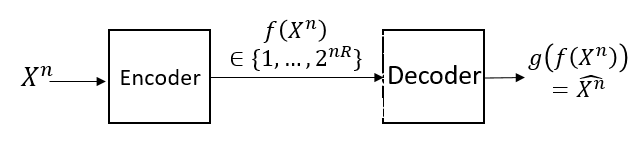
A distortion function $d:\mathcal{X}\times\mathcal{X}\to\mathbb{R}^{+}$ quantifies the difference of the original and reconstructed message. Distortion between sequence $X^{n}$ and $\hat{X}^{n}$ is defined as the average distortion of $X_{i}$’s and $\hat{X}_{i}$’s. Commonly used distortion function includes Hamming distortion function $d(x,\hat{x})=\mathbbm{1}[x\neq\hat{x}]$ for $\mathcal{X}=\{0,1\}$ and square distortion function $d(x,\hat{x})=(x-\hat{x})^{2}$ for $\mathcal{X}=\mathbb{R}$.

Now we are ready to define the rate-distortion function for data compression.

The main theorem of rate-distortion theory (Cover and Thomas, (2012, Theorem 10.2.1)) states as follows,

The rate distortion quantifies the fundamental limit of data compression, i.e., at least how many bits are needed to compress the data, given the quality of the reconstructed data. Here is an example for rate-distortion function.

If the required distortion $D$ is larger than the variance of the Gaussian variable $\sigma^{2}$, we simply transmit $\hat{X}=0$; otherwise, we will transmit $\hat{X}$ such that $\hat{X}\sim\mathcal{N}(0,\sigma^{2}-D)$, $X-\hat{X}\sim\mathcal{N}(0,D)$ where $\hat{X}$ and $X-\hat{X}$ are independent.

Now we extend the rate distortion theory for data compression to model compression. To apply the rate distortion theory to model compression, we view the weights in the model as a multi-dimensional random variable $W\in\mathbb{R}^{m}$ following distribution $P_{W}$. The randomness comes from multiple sources including different distributions of training data, randomness of training data and randomness of training algorithm. The compressor can also be random hence we describe the compressor by a conditional probability $P_{\hat{W}|W}$. Now we define the distortion and rate in model compression, analogously to the data compression scenario.

Distortion. Assume we have a neural network $f_{w}$ that maps input $x\in\mathbb{R}^{d_{x}}$ to $f_{w}(x)$ in output space $\mathcal{S}$. For regressors, $f_{w}(x)$ is defined as the output of the neural network on $\mathbb{R}^{d_{y}}$. Analogous to the square distortion in data compression, We define the distortion to be the expected $\ell_{2}$ distance between $f_{w}$ and $f_{\hat{w}}$, i.e.

For classfiers, $f_{w}(x)$ is defined as the output probability distribution over $C$ classes on the simplex $\Delta^{C-1}$. We define the distortion to be the expected distance between $f_{w}$ and $f_{\hat{w}}$, i.e.

Here $D$ could be any statistical distance, including KL divergence, Hellinger distance, total variation distance, etc. Such a definition of distortion captures the difference between the original model and the compressed model, averaged over data $X$, and measures the quality of a compression algorithm.

Rate. In data compression, the rate is defined as the description length of the bits necessary to communicate the compressed data $\hat{X}$. The compressor outputs $\hat{X}$ from a finite code book $\mathcal{X}$. The description consists the code word which are the indices of $\hat{x}$ in the code book, and the description of the code book.

In rate distortion theory, we ignore the code book length. Since we are transmitting a sequence of data $X^{n}$, the code word has to be transmitted for each $X_{i}$ but the code book is only transmitted once. In asymptotic setting, the description length of code book can be ignored, and the rate is defined as the description length of the code word.

In model compression, we also define the rate as the code word length, by assuming that an underlying distribution $P_{W}$ of the parameters exists and infinitely many models whose parameters are i.i.d. from $P_{W}$ will be compressed. In practice, we only compress the parameters once so there is no distribution of the parameters. Nevertheless, the rate distortion theory can also provide important intuitions for one-time compression, explained in Section 5.

Now we can define the rate distortion function for model compression. Analogously to Theorem 1, the rate distortion function for model compression is defined as follows,

In the following sections we establish a lower bound of the rate-distortion function.

Assume that we are going to compress a linear regression model $f_{w}(x)=w^{T}x$. We assume that the mean of data $x\in\mathbb{R}^{m}$ is zero and the covariance matrix is diagonal, i.e., $\mathbb{E}_{X}[X_{i}^{2}]=\lambda_{x,i}>0$ and $\mathbb{E}_{X}[X_{i}X_{j}]=0$ for $i\neq j$. Furthermore, assume that the parameters $W\in\mathbb{R}^{m}$ are drawn from a Gaussian distribution $\mathcal{N}(0,\Sigma_{W})$. The following theorem gives the lower bound of the rate distortion function for the linear regression model.

This lower bound gives rise to a “weighted water-filling” approach, which differs from the classical “water-filling” for rate distortion of colored Gaussian source in Cover and Thomas, (2012, Figure 13.7). The details and graphical explanation of the “weighted water-filling” can be found in Appendix A.

We show that, the lower bound give in Theorem 2 is achievable. Precisely, we have the following theorem.

The optimal compressor is Algorithm 1 in Appendix A. Intuitively, the optimal compressor does the following

• •

  Find the optimal water levels $D_{i}$ for “weighted water filling”, such that the expected distortion $D=\mathbb{E}_{W,\hat{W}}[d(W,\hat{W})]=\mathbb{E}_{W,\hat{W}}[\hat{W}^{T}\Sigma_{X}(W-\hat{W})]$ is minimized given certain rate.

• •

  Add a noise $Z_{i}$ which is independent of $\hat{W}_{i}=W_{i}+Z_{i}$ and has a variance proportional to the water level. That is possible since $W$ is Gaussian.

We can check that the compressor makes all the inequalities become equality, hence achieve the lower bound. The full proof of the lower bound and achievability can be found in Appendix A.

Recall that for linear regression model, to achieve the smallest rate given certain distortion (or, equivalently, achieve the smallest distortion given certain rate), the optimal compressor need to do the following: (1) find appropriate “water levels” such that the expected distortion $E_{W,\hat{W}}[d(W,\hat{W})]=\mathbb{E}_{W,\hat{W},X}[(W^{T}X-\hat{W}^{T}X)^{2}]=\mathbb{E}_{W,\hat{W}}[(W-\hat{W})^{T}\Sigma_{X}(W-\hat{W})]$ is minimized. (2) make sure that $\hat{W}_{i}$ is independent with $W_{i}-\hat{W}_{i}$, in other words, $\mathbb{E}_{W,\hat{W}}[\hat{W}^{T}\Sigma_{X}(W-\hat{W})]=0$. Hence, we extract the following two “golden rules”:

1. 1.

   $\mathbb{E}_{W,\hat{W}}[\hat{W}^{T}\Sigma_{X}(W-\hat{W})]=0$

2. 2.

   $\mathbb{E}_{W,\hat{W}}[(W-\hat{W})^{T}\Sigma_{X}(W-\hat{W})]$ should be minimized, given certain rate.

For practical model compression, we adopt these two “golden rules”, by making the following amendments. First, we discard the expectation over $W$ and $\hat{W}$ since there is only one model to be compressed. Second, the distortion can be written as $d(w,\hat{w})=(w-\hat{w})^{T}\Sigma_{X}(w-\hat{w})$ only for linear models. For non-linear models, the distortion function is complicated, but can be approximated by a simpler formula. For non-linear regression models, we take first order Taylor expansion of the function $f_{\hat{w}}(x)\approx f_{w}(x)+(\hat{w}-w)^{T}\nabla_{w}f_{w}(x)$, and have

where the “weight importance matrix” defined as

quantifies the relative importance of each weight to the output. For linear regression models, weight importance matrix $I_{w}$ equals to $\Sigma_{X}$.

For classification models, we will first approximate the KL divergence. Using the Taylor expansion $x\log(x/a)\approx(x-a)+(x-a)^{2}/(2a)$ for $x/a\approx 1$, the KL divergence $D_{KL}(P||Q)$ for can be approximated by $D_{KL}(P||Q)\approx\sum_{i}(P_{i}-Q_{i})+(P_{i}-Q_{i})^{2}/(2P_{i})=\sum_{i}(P_{i}-Q_{i})^{2}/(2P_{i})$, or in vector form $D_{KL}(P||Q)\approx\frac{1}{2}(P-Q)^{T}{\rm diag}[P^{-1}](P-Q)$. Therefore,

So the weight importance matrix is given by

This weight importance matrix is also valid for many other statistical distances, including reverse KL divergence, Hellinger distance and Jenson-Shannon distance.

Now we define the two “golden rules” for practical model compression algorithms,

1. 1.

   $\hat{w}^{T}I_{w}(w-\hat{w})=0$,

2. 2.

   $(w-\hat{w})^{T}I_{w}(w-\hat{w})$ is minimized given certain constraints.

In the following subsection we will show the optimality of the “golden rules” for a one-hidden-layer neural network.

We show that if a compressor of a one-hidden-layer ReLU network satisfies the two “golden rules”, it will be the optimal compressor, with respect to mean-square-error. Precisely, consider the one-hidden layer ReLU neural network $f_{w}(x)=ReLU(w^{T}x)$, where the distribution of input $x\in\mathbb{R}^{m}$ is $\mathcal{N}(0,\Sigma_{X})$. Furthermore, we assume that the covariance matrix $\Sigma_{X}={\rm diag}[\lambda_{x,1},\dots,\lambda_{x,m}]$ is diagonal and $\lambda_{x,i}>0$ for all $i$. We have the following theorem.

The proof uses the techniques of Hermite polynomials and Fourier analysis on Gaussian spaces, inspired by Ge et al., (2017). The full proof can be found in Appendix B.

Here $\hat{\mathcal{W}}$ denotes a class of compressors, with some constraints. For example, $\hat{\mathcal{W}}$ could be the class of pruning algorithms where no more than 50% weights are pruned, or $\hat{\mathcal{W}}$ could be the class of quantization algorithm where each weight is quantized to 4 bits. Theoretically, it is not guaranteed that the two “golden rules” can be satisfied simultaneously for every $\hat{\mathcal{W}}$, but in the following subsection we show that they can be satisfied simultaneously for two of the most commonly used class of compressors — pruning and quantization. Hence, minimizing the objective $(w-\hat{w})^{T}I_{w}(w-\hat{w})$ will be optimal for pruning and quantization.

Pruning and quantization are two most basic and useful building blocks of modern model compression algorithms, For example, DeepCompress Han et al., 2015a () iteratively prune, retrain and quantize the neural network and achieve state-of-the-art performances on large neural networks.

In pruning algorithms, we choose a subset $S\in[m]$ and set $\hat{w}_{i}=0$ for all $i\in S$ and $\hat{w}_{i}=w_{i}$ for $i\not\in S$. The compression ratio is evaluated by the proportion of unpruned weights $r=(m-|S|)/m$. Since either $\hat{w}_{i}$ or $w_{i}-\hat{w}_{i}$ is zero, so the first “golden rule” is automatically satisfied, so we have the following corollary.

In quantization algorithms, we cluster the weights into $k$ centroids $\{c_{1},\dots,c_{k}\}$. The algorithm optimize the centroids as long as the assignments of each weight $A_{i}\in[k]$. The final compressed weight is given by $\hat{w}_{i}=c_{A_{i}}$. Usually $k$-means algorithm are utilized to minimize the centroids and assignments alternatively. The compression ratio of quantization algorithm is given by

where $m$ is the number of weights and $b$ is the number of bits to represent one weight before quantization (usually 32). By using Huffman coding, the average number of bits for each weight is given by $\sum_{j=1}^{k}(m_{j}/m)\lceil\log_{2}(m/m_{j})\rceil$, where $m_{j}$ is the number of weights assigned to the $j$-th cluster.

If we can find the optimal quantization algorithm with respect to $(w-\hat{w})^{T}I_{w}(w-\hat{w})$, then each centroids $c_{j}$ should be optimal, i.e.

where $e_{i}$ is the $i$-th standard basis. Therefore, we have

Hence the first “golden rule” is satisfied if the second “golden rule” is satisfied. So we have

As corollaries of Theorem 4, we proposed to use $(w-\hat{w})^{T}I_{w}(w-\hat{w})$ as the objective for pruning and quantization algorithms, which can achieve the minimum MSE for one-hidden-layer ReLU neural network.

Recall that for classification problems, the weight importance matrix is defined as

For computational simplicity, we drop the off-diagonal terms of $I_{w}$, and simplify the objective to
$\sum_{i=1}^{m}\mathbb{E}_{X}[\frac{(\nabla_{w_{i}}f_{w}(X))^{2}}{f_{w}(X)}](w_{i}-\hat{w}_{i})^{2}$. To minimize the proposed objective, a pruning algorithm just prune the weights with smaller $\mathbb{E}_{X}[\frac{(\nabla_{w_{i}}f_{w}(X))^{2}}{f_{w}(X)}]w_{i}^{2}$ greedily. A quantization algorithm uses the weighted $k$-means algorithm Choi et al., (2016) to find the optimal centroids and assignments. We compare the proposed objective with the baseline objective $\sum_{i=1}^{m}(w_{i}-\hat{w}_{i})^{2}$, which were used as building blocks in DeepCompress Han et al., 2015a (). We compare the objectives in Table 1.

For pruning experiment, we choose the same compression rate for every convolutional layer and fully-connected layer, and plot the test accuracy and test cross-entropy loss against compression rate. For quantization experiment, we choose the same number of clusters for every convolutional and fully-connected layer. Also we plot the test accuracy and test cross-entropy loss against compression rate. To reduce the variance of estimating the weight importance matrix $I_{w}$, we use the temperature scaling method introduced by Guo et al., (2017) to improve model calibration.

We show that results of pruning experiment in Figure 2, and the results of quantization experiment in Figure 3. We can see that the proposed objective gives better validation cross-entropy loss than the baseline, for every different compression ratios. The proposed objective also gives better validation accuracy in most scenarios. We relegate the results for CIFAR100 in Appendix C.

In the previous experiment, we only use the training data to compute the weight importance matrix. But if we can use the training label as well, we can further improve the performance of pruning and quantization algorithms. If the training label is available, we can view the cross-entropy loss function $\mathcal{L}(f_{w}(x),y)=\mathcal{L}_{w}(x,y)$ as a function from $\mathcal{X}\times\mathcal{Y}\to\mathbb{R}^{+}$, and define the distortion function as

Taking first order approximation of the loss function gives the supervised weight importance matrix,

We write $\mathbb{E}$ instead of $\mathbb{E}_{X,Y}$ for simplicity. Similarly, we drop the off-diagonal terms for ease of computation, and simplify the objective to $\sum_{i=1}^{m}\mathbb{E}[(\nabla_{w_{i}}\mathcal{L}_{w}(X,Y))^{2}](w_{i}-\hat{w}_{i})^{2}$, which is called gradient-based objective. Note that for well-trained model, the expected value of gradient $\mathbb{E}[\nabla_{w}\mathcal{L}_{w}(X,Y)]$ is closed to zero, but the second moment of the gradient $\mathbb{E}[\nabla_{w}\mathcal{L}_{w}(X,Y)(\nabla_{w}\mathcal{L}_{w}(X,Y))^{T}]$ could be large. We compare this objective with the baseline objective $\sum_{i=1}^{m}(w_{i}-\hat{w}_{i})^{2}$. We also compare with the hessian-based objective $\sum_{i=1}^{m}\mathbb{E}[\nabla^{2}_{w_{i}}\mathcal{L}_{w}(X,Y)](w_{i}-\hat{w}_{i})^{2}$, which is used in LeCun et al., (1990) and Hassibi and Stork, (1993) for network pruning and Choi et al., (2016) for network quantization. To estimate the diagonal entries of the Hessian matrix of the loss function with respect to the model parameters, we implemented Curvature Propagation Martens et al., (2012) treating each layer and activation as a node. The running time is proportional to the running time of the usual gradient back-propagation by a factor that does not depend on the size of the model. Manually optimizing the local Hessian calculation at each node reduces memory usage and allows us to use larger batch size and larger number of samples for more accurate estimates.

Furthermore, if we take second order approximation of the loss function, and drop the off-diagonal terms of the squared gradient matrix and squared hessian tensor, we have the following approximation

which is called gradient+hessian based objective. For pruning algorithm, we can prune the weights with smaller $\mathbb{E}[(\nabla_{w_{i}}\mathcal{L}_{w}(X,Y))^{2}]w_{i}^{2}+\frac{1}{4}\mathbb{E}[(\nabla^{2}_{w_{i}}\mathcal{L}_{w}(X,Y))^{2}]w_{i}^{4}$ greedily. For quantization algorithm, we use an alternatice minimization algorithm in Appendix C to find the minimum. We conclude the different supervised objectives in Table 2.

We show that results of pruning experiment in Figure 4, and the results of quantization experiment in Figure 5. Generally, the gradient objective and hessian objective both give better performance than baseline objective , while gradient objective is slightly than hessian objective at some points. Gradient + hessian objective gives the best overall performance. We relegate the results for CIFAR100 in Appendix C.

Remark. Here we define the supervised distortion function as $d(w,\hat{w})=\mathbb{E}_{X,Y}\left[(\mathcal{L}_{w}(X,Y)-\mathcal{L}_{\hat{w}}(X,Y))^{2}\right]$, analogously to the distortion of regression. However, since the goal of classification is to minimize the loss function, the following definition of distortion function $\tilde{d}(w,\hat{w})=\mathbb{E}_{X,Y}\left[\mathcal{L}_{\hat{w}}(X,Y)-\mathcal{L}_{w}(X,Y)\right]$ is also valid and has been adopted in LeCun et al., (1990) and Choi et al., (2016). The main difference is — $d(w,\hat{w})$ focus on the quality of compression algorithm, i.e., how similar is the compressed model compared to uncompressed model, whereas $\tilde{d}(w,\hat{w})$ focus on the quality of compressed model, i.e. how good is the compressed model. So $d(w,\hat{w})$ is a better criteria for the compression algorithm. Additionally, by taking second order approximation of $d(w,\hat{w})$, we have gradient+hessian objective, which shows better empirical performance than hessian objective, derived by taking second order approximation of $\tilde{d}(w,\hat{w})$.

References

- Berger, (1971) Berger, T. (1971). Rate distortion theory: A mathematical basis for data compression.
- Cao et al., (2018) Cao, W., Wang, X., Ming, Z., and Gao, J. (2018). A review on neural networks with random weights. Neurocomputing, 275:278–287.
- Chen et al., (2015) Chen, W., Wilson, J., Tyree, S., Weinberger, K., and Chen, Y. (2015). Compressing neural networks with the hashing trick. In International Conference on Machine Learning, pages 2285–2294.
- Cheng et al., (2015) Cheng, Y., Yu, F. X., Feris, R. S., Kumar, S., Choudhary, A., and Chang, S.-F. (2015). An exploration of parameter redundancy in deep networks with circulant projections. In Proceedings of the IEEE International Conference on Computer Vision, pages 2857–2865.
- Choi et al., (2016) Choi, Y., El-Khamy, M., and Lee, J. (2016). Towards the limit of network quantization. arXiv preprint arXiv:1612.01543.
- Coates et al., (2013) Coates, A., Huval, B., Wang, T., Wu, D., Catanzaro, B., and Andrew, N. (2013). Deep learning with cots hpc systems. In International Conference on Machine Learning, pages 1337–1345.
- Cover and Thomas, (2012) Cover, T. M. and Thomas, J. A. (2012). Elements of information theory. John Wiley & Sons.
- Denton et al., (2014) Denton, E. L., Zaremba, W., Bruna, J., LeCun, Y., and Fergus, R. (2014). Exploiting linear structure within convolutional networks for efficient evaluation. In Advances in neural information processing systems, pages 1269–1277.
- Federici et al., (2017) Federici, M., Ullrich, K., and Welling, M. (2017). Improved bayesian compression. arXiv preprint arXiv:1711.06494.
- Ge et al., (2017) Ge, R., Lee, J. D., and Ma, T. (2017). Learning one-hidden-layer neural networks with landscape design. arXiv preprint arXiv:1711.00501.
- Gong et al., (2014) Gong, Y., Liu, L., Yang, M., and Bourdev, L. (2014). Compressing deep convolutional networks using vector quantization. arXiv preprint arXiv:1412.6115.
- Guo et al., (2017) Guo, C., Pleiss, G., Sun, Y., and Weinberger, K. Q. (2017). On calibration of modern neural networks. arXiv preprint arXiv:1706.04599.
- (13) Han, S., Mao, H., and Dally, W. J. (2015a). Deep compression: Compressing deep neural networks with pruning, trained quantization and huffman coding. arXiv preprint arXiv:1510.00149.
- (14) Han, S., Pool, J., Tran, J., and Dally, W. (2015b). Learning both weights and connections for efficient neural network. In Advances in neural information processing systems, pages 1135–1143.
- Hanson and Pratt, (1989) Hanson, S. J. and Pratt, L. Y. (1989). Comparing biases for minimal network construction with back-propagation. In Advances in neural information processing systems, pages 177–185.
- Hassibi and Stork, (1993) Hassibi, B. and Stork, D. G. (1993). Second order derivatives for network pruning: Optimal brain surgeon. In Advances in neural information processing systems, pages 164–171.
- He et al., (2018) He, Y., Lin, J., Liu, Z., Wang, H., Li, L.-J., and Han, S. (2018). Amc: Automl for model compression and acceleration on mobile devices.
- Howard et al., (2017) Howard, A. G., Zhu, M., Chen, B., Kalenichenko, D., Wang, W., Weyand, T., Andreetto, M., and Adam, H. (2017). Mobilenets: Efficient convolutional neural networks for mobile vision applications. arXiv preprint arXiv:1704.04861.
- Iandola et al., (2016) Iandola, F. N., Han, S., Moskewicz, M. W., Ashraf, K., Dally, W. J., and Keutzer, K. (2016). Squeezenet: Alexnet-level accuracy with 50x fewer parameters and¡ 0.5 mb model size. arXiv preprint arXiv:1602.07360.
- Jiao et al., (2017) Jiao, J., Gao, W., and Han, Y. (2017). The nearest neighbor information estimator is adaptively near minimax rate-optimal. arXiv preprint arXiv:1711.08824.
- Krizhevsky et al., (2012) Krizhevsky, A., Sutskever, I., and Hinton, G. E. (2012). Imagenet classification with deep convolutional neural networks. In Advances in neural information processing systems, pages 1097–1105.
- LeCun et al., (1998) LeCun, Y., Bottou, L., Bengio, Y., and Haffner, P. (1998). Gradient-based learning applied to document recognition. Proceedings of the IEEE, 86(11):2278–2324.
- LeCun et al., (1990) LeCun, Y., Denker, J. S., and Solla, S. A. (1990). Optimal brain damage. In Advances in neural information processing systems, pages 598–605.
- Louizos et al., (2017) Louizos, C., Ullrich, K., and Welling, M. (2017). Bayesian compression for deep learning. In Advances in Neural Information Processing Systems, pages 3288–3298.
- Mandt et al., (2017) Mandt, S., Hoffman, M. D., and Blei, D. M. (2017). Stochastic gradient descent as approximate bayesian inference. The Journal of Machine Learning Research, 18(1):4873–4907.
- Martens et al., (2012) Martens, J., Sutskever, I., and Swersky, K. (2012). Estimating the hessian by back-propagating curvature. arXiv preprint arXiv:1206.6464.
- McDonald and Schultheiss, (1964) McDonald, R. and Schultheiss, P. (1964). Information rates of gaussian signals under criteria constraining the error spectrum. Proceedings of the IEEE, 52(4):415–416.
- Shannon, (1959) Shannon, C. E. (1959). Coding theorems for a discrete source with a fidelity criterion. IRE Nat. Conv. Rec, 4(142-163):1.
- Silver et al., (2017) Silver, D., Schrittwieser, J., Simonyan, K., Antonoglou, I., Huang, A., Guez, A., Hubert, T., Baker, L., Lai, M., Bolton, A., et al. (2017). Mastering the game of go without human knowledge. Nature, 550(7676):354.
- Simonyan and Zisserman, (2014) Simonyan, K. and Zisserman, A. (2014). Very deep convolutional networks for large-scale image recognition. arXiv preprint arXiv:1409.1556.
- Ullrich et al., (2017) Ullrich, K., Meeds, E., and Welling, M. (2017). Soft weight-sharing for neural network compression. arXiv preprint arXiv:1702.04008.
- Vanhoucke et al., (2011) Vanhoucke, V., Senior, A., and Mao, M. Z. (2011). Improving the speed of neural networks on cpus. In Proc. Deep Learning and Unsupervised Feature Learning NIPS Workshop, volume 1, page 4. Citeseer.
- Wu et al., (2016) Wu, Y., Schuster, M., Chen, Z., Le, Q. V., Norouzi, M., Macherey, W., Krikun, M., Cao, Y., Gao, Q., Macherey, K., et al. (2016). Google’s neural machine translation system: Bridging the gap between human and machine translation. arXiv preprint arXiv:1609.08144.
Appendix A Lower bound for rate distortion function
In this section, we finish the proof of the lower bound and achievability in Section 4. Our approach is based on the water-filling approach McDonald and Schultheiss, (1964).
A.1 General lower bound
First, we establish establishes a lower bound of the rate distortion function, which works for general models..
Lemma 1
The rate-distortion function , where is the optimal value of the following optimization problem.
where is the differential entropy of and is the differential entropy of the -th entry of .
A.1.1 Proof of Lemma 1
Recall that the rate distortion function for model compression is defined as . Now we lower bound the mutual information by
Here the last inequality comes from the fact that conditioning does not increase entropy. Notice that the first term does not depend on the compressor. For the last term, we upper bound each term in two ways. On one hand, is upper bounded by because conditioning does not increase entropy. On the other hand, , and by Cover and Thomas, (2012, Theorem 8.6.5), differential entropy is maximized by Gaussian distribution, for given second moment. We then have:
Therefore, the lower bound of the mutual information is given by,
A.2 Lower bound for linear model
For complex models, the general lower bound in Lemma 1 is difficult to evaluate, due to the large dimension of parameters. It was shown by Jiao et al., (2017) that the sample complexity to estimate differential entropy is exponential to the dimension. It’s even harder to design an algorithm to achieve the lower bound. But for linear model, the lower bound can be simplified. For , the distortion function can be written as
Since we assumed that , and , so the constraint in Lemma 1 is given by
Then the optimization problem in Lemma 1 can be written as follows
Here is a Gaussian random variable, so . The Lagrangian function of the problem is given by
By setting the derivative w.r.t. to 0, we have
for all such that . So the optimal should satisfy that is constant, for all such that . Also the optimal is at most . Also, since the lower bound is given by
where
where is chosen that .