Analog Models for Holographic Transport
Abstract
The gauge-gravity duality and analog gravity both relate a condensed matter system to a gravitational theory. This makes it possible to use gravity as an intermediary to establish a relation between two different condensed matter systems: The strongly coupled system from the gauge-gravity duality and the weakly coupled gravitational analog. We here offer some examples for relations between observables in the two different condensed matter systems. In particular, we show that in some cases Green’s functions and first order transport coefficients in holographic models are of the same form as those in an analog gravitational system, which allows in principle to obtain the former by measuring the latter.
1 Introduction
The AdS/CFT correspondence [1, 2, 3] relates certain conformal field theories (CFTs) with quantum gravitational models that arise in string theory. The latter, gravitational, theory describes a space-time with negative cosmological constant, the so-called Anti-de Sitter space-time (AdS), while the former CFT is located on the conformal boundary of AdS, i.e. in a space-time with one spacial dimension less.
The most intriguing feature of the AdS/CFT correspondence is that when one of the theories is strongly coupled, then the other is weakly coupled and vice versa. Especially useful for practical purposes is the limit when string effects and quantum effects are both negligible and the CFT is strongly coupled while the gravitational theory is weakly coupled. In this limit, certain gravitational theories can be used as effective models for strongly coupled condensed matter systems, a technique that can still be applied when the usual methods of quantum field theory fail. (See e.g. [4, 5, 6] for reviews.)
Intriguingly, there is another approach where a curved space-time emerges in the description of condensed matter systems, and that is analog gravity. Analog gravity is based on the observation that small perturbations around a background medium are described by an equation of motion which is formally identical to that of fields propagating in a curved space-time. Analog gravity hence links weakly coupled gravity with a weakly coupled condensed matter system. The relations underlying analog gravity have been known since the mid 1980s [7, 8] but only in recent years has the topic begun to attract attention, quite possibly because experimental realization has become more feasible [9, 10, 11, 12, 13, 14].
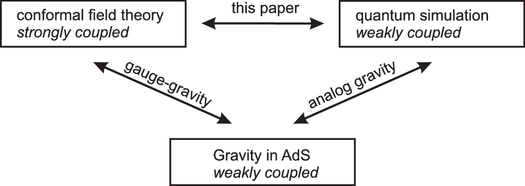
Seeing the evident similarities, it lies at hand that one tries to combine both relations – AdS/CFT and analog gravity – to arrive at a relation between two condensed matter systems. This can be done because AdS/CFT and analog gravity both use a curved geometry as an effective description for a condensed matter system, but the one condensed matter system is strongly coupled and the other one is weakly coupled (see Figure 1). The combination of both relations then – the “analog duality” [15, 16] – links a strongly coupled with a weakly coupled condensed matter system.
In analog duality, the curved space-time merely constitutes a mathematical framework by help of which computations can be performed. It has no direct correspondence to the actual space-time geometry in which the condensed matter systems are situated (usually assumed to be flat space). Nevertheless, this effective geometry can be employed as a mathematical intermediary between the two different condensed matter systems, which will then, in certain aspects, be dual to each other, meaning that quantities in the one description can be identified with quantities in the other description. The purpose of this paper is to present some examples for the, so derived, relations between observables in different condensed matter systems.
This topic that has been approached from various angles in the last years [17, 18, 19, 20, 21, 15, 16] and ties into the overarching scheme of quantum simulation (see e.g. [22]). The aim of quantum simulations is to custom-design systems which mimic the behavior of a different, mathematically intractable, situation, and then measure the results rather than calculate them. The AdS/CFT duality does not lend itself to this purpose because the gravitational dual does not represent a real-world situation and cannot be simulated in the laboratory. If the gravitational dual, however, is further mapped onto an analog gravity system, then we are dealing with a correspondence of which both sides are experimentally accessible, thereby making quantum simulation possible.
The application that we will focus on in this present work is the calculation of Green functions and first-order transport coefficients. In holography, we have a straightforward procedure to compute these quantities from solutions of a system of partial differential equations in a curved background geometry [23]. Mathematically, this is exactly the type of equations which one also has in analog gravity.
The task thus comes down to finding a pair of an analog gravity system and a holographic dual of another system for which the background geometries are identical. Then the two models have a one-to-one correspondence that maps transport coefficients and Green functions of the holographic model to perturbations of the analog gravity system, provided boundary conditions are chosen appropriately. This means any experiment that realizes the suitable analog gravity system can then be employed as an analog dual to compute transport properties in the strongly correlated condensed matter systems with the corresponding holographic dual.
The paper is organized as follows. In order to be self-contained, sections 2 and 3 provide short summaries of the aspects of analog gravity and holography that are relevant for what follows. In section 4 we present several examples which illustrate how transport coefficients can be determined by the solution of a scalar field in a curved geometry. In section 5 we discuss how the results presented here can be generalized.
Units are chosen such that the speed of light and . The reader be warned that denotes the speed of sound in the analog model and not the speed of light. Our metric convention is the ‘mostly plus’ signature, .
2 Analog Gravity
We begin with briefly summarizing the key idea of analog gravity. Consider we have a complex scalar field with Lagrangian
| (1) |
Here and in the following we will allow the potential to have an explicit coordinate dependence because we have in mind interactions that are designed in the laboratory. Such interactions are typically induced by the presence of external fields [24] and are chosen for the very purpose of creating a specific quantum simulation. We assume that the potential breaks the global symmetry in a stable minimum. This minimum will define our background field. is the background metric of the space-time in which the field resides and is assumed to be the Minkowski-metric.
The complex scalar field can be expressed in terms of two real scalar fields as , so that the Lagrangian takes the form
| (2) |
We can then derive the equation of motion for
| (3) |
where
| (4) |
is the kinetic term of the phase-field . Assuming that the left hand side of (3) is negligibly small, we solve this equation to express as a function of and insert this back into the Lagrangian. This will generically result in an effective Lagrangian for of the form
| (5) |
In particular, if the original potential was polynomial in , the resulting Lagrangian will contain some (in general fractional) power of . This is a good effective theory so long as the classical equations of motion are approximately valid and is slowly varying. It is a common limit to use in the treatment of Bose–Einstein condensates.
For the analog gravitational system will denote with a background field that solves the Euler–Lagrange equations for (5) and then consider a fluctuation around this solution,
| (6) |
Demanding that this expansion again solves the Euler–Lagrange equations leads to equations of motion for the fluctuations when expanding in orders of [8]. Focusing on the lowest order fluctuation, the equation of motion can be brought into the form
| (7) |
where the (inverse of the) “acoustic metric” is defined as
| (8) |
and the “effective mass” of the perturbation is
| (9) |
The significance of (7) is that this is the exact same equation which also describes the propagation of a field in a curved geometry with metric . As a consequence, fluctuations in a condensed matter system can be used to simulate physics in curved space-time even though the ‘real’ space-time in which the system is located remains flat.
Note that if the potential in (1) did respect the global U(1) symmetry, then the perturbation will be massless, as is expected for the Goldstone boson. One can, however, generate masses for by explicitly breaking the U(1) symmetry. This corresponds to the familiar ‘tilt’ of the potential that e.g. gives masses to pions due to the breaking of chiral symmetry. We will make use of this explicit symmetry breaking later on.
For practical purposes, it is often useful to rewrite (8) in quantities that are more commonly used for gases and fluids. For this one notes that the Lagrange density (5) defines a stress-energy-tensor,
| (10) |
This can be rewritten as the stress stress-energy-tensor of a fluid,
| (11) |
where four-velocity, pressure, and density of the background field are given by
| (12) |
such that the four-velocity is normalized as it should
| (13) |
The field equations of the relativistic fluid are then identical to the conservation of the stress energy
| (14) |
and the acoustic metric and its inverse can be expressed as
| (15) | |||||
| (16) |
Here, is the speed of sound and defined by .
In the non-relativistic limit one has and and then the acoustic metric is of the form
In this limit, the equations of motion for the background field are the familiar continuity equation and the Euler equation:
| (23) | |||||
| (24) |
If the fluid is non-viscous, has vanishing rotation (i.e. is vorticity-free), and is barotropic, we can further simplify this expression. The velocity field is then the gradient of a scalar field and the density is a function of only. In this case, the Euler equation can be integrated once and then be written as
| (25) |
where
| (26) |
is the specific enthalpy.
3 The Holographic Dictionary
In this section we will summarize how the AdS/CFT correspondence connects observables of the boundary CFT with the gravitational theory in the bulk. In section 4 we will then go through these observables again and further connect them with observables of the analog gravity system.
Since the CFT is located on the boundary of the space-time in which the gravitational theory operates, the AdS/CFT correspondence is frequently referred to as “holographic”. Holography relates a gravitational theory, i.e. one with dynamical geometry, in dimensions to a non-gravitational field theory in dimensions.
Because the dimensional bulk is an AdS space-time, it is not globally hyperbolic. This means that initial conditions on a space-like slice do not uniquely determine the propagation of fields in this space-time. For a problem to be well-defined, therefore, initial conditions have to be supplemented by additional conditions on the conformal boundary when approaching spacial infinity. This means that the key ingredient of holography is to convert the computation of observables in the strongly coupled CFT on the boundary into a boundary value problem in the curved geometry of the bulk.
We can picture the field theory dual as ‘living on the boundary’ since its degrees of freedom are given by the asymptotic behavior of the bulk fields. Schematically, using to denote the collection of all bulk fields, including the geometry, the boundary degrees of freedom are obtained from asymptotic scaling relations of the form
| (27) |
where the exponent depends on the field and is the bulk-coordinate in AdS which approaches zero at the boundary.
In the dual field theory, these are sources that couple to an operator , and their correlation functions are evaluated as
| (28) |
Another way to say this is that the gravitational action
| (29) |
evaluated “on-shell”, i.e. on a solution of the corresponding Euler-Lagrange equations, serves as the generating functional of connected correlators of the field theory dual. The exponents in (27) are then related to the conformal dimension of the corresponding operators .
Evaluating (28) may, at first sight, appear uselessly difficult, given that the equations of motion in systems with dynamical geometry are highly non-linear and explicit solutions for arbitrary boundary conditions are in general not known analytically. What makes the formula useful, though, is that it can be evaluated perturbatively. That is, when a specific background is chosen, then the -point functions can be calculated by making a perturbative expansion up to order .
For this to work we assume that the equations of motion are Hamiltoinian11 1 Even higher derivative theories can usually be brought to the form (29) and having a Hamiltonian functional is generally to be expected in physically realistic systems, so that a particular solution is entirely characterized by , where are the conjugate momenta to the fields . The momenta can be expressed in terms of boundary values of derivatives of the bulk fields , but can as well be identified using the standard relation
| (30) |
A specific solution to the equation of motion is selected by fixing on a characteristic surface – usually at the AdS boundary – which gives rise to relation of the type
| (31) |
Next, one makes a perturbative expansion of the bulk fields around the background solution
| (32) |
This induces an expansion of the momenta in terms of the boundary fields which has the general form
| (33) |
The coefficients in this expansion then correspond to the -point correlation functions from (28). The special case of the -point function corresponds to the holographic Green function , which will be discussed further in sections 4.2 and 4.3.
The details of the relation (33) depend on the properties of the space of solutions in which one studies a particular problem or configuration. This often means that we must apply further consistency-conditions in the bulk. Usually, these are condition like demanding that the bulk geometry is smooth or that curvature singularities are hidden behind a regular event horizon (the latter to ensure that the geometry remains non-singular when time is Wick-rotated to Euclidean signature). In such cases, the consistency conditions in the bulk usually boil down to a set of boundary conditions at the event horizon.
The most straight-forward aspects of the correspondence relate the metric in the bulk with properties of the theory on the boundary. Of particular interest are space-times with an event horizon (in the following referred to as black hole space-times) because their duals describe strongly coupled CFTs at finite temperature.
In such a case, if the AdS-space contains a black hole, then the Hawking temperature associated with the black hole horizon via the surface gravity corresponds to the temperature of the CFT on the boundary. The entropy density of both systems is the same. From the metric in the bulk one can further extract the stress-energy-tensor on the boundary with a suitable renormalization procedure that strips off the infinites which the asymptotic limit brings [25].
4 The New Dictionary of Analog Duality
We here consider a model that has been widely used in the literature as a phenomenological to study electric transport, in particular in holographic superconductors [26, 4]. It consists of a scalar field, , which is charged under a gauge field, , and minimally coupled to Einstein gravity,
| (34) | |||||
The equations of motion from this action are a combination of Einstein’s field equations, the Maxwell equation and a Klein–Gordon equation for the scalar field,
| (35) | |||||
| (36) | |||||
| (37) |
With the usual stress-energy tensors for the field stength and a charged scalar, respectively,
| (38) | |||||
| (39) |
and the current
| (40) |
A frequently studied background solution of these equations are time-independent space-time geometries with translational symmetry in the transverse directions, such that the metric can be parametrized as
| (41) |
where is the typical length scale in the bulk and the coordinate goes to zero on the AdS conformal boundary. For later convenience, we also introduce a frame, , adapted to the diagonal form of the metric,
| (42) |
In this case is also a function of olny, , and the gauge field is of the form
| (43) |
Explicit expressions for in closed form are only known for , when the metric reduces to the AdS Reissner-Nordström space-time, which is given by
| (44) |
In the following we focus mostly on the simple action (34) as an illustrative example, we wish to emphasize that it was shown in [27] that any metric of the form (41) can be realized as an analog metric.
4.1 Background values
To illustrate the general idea, we will start with some simple examples that build on the previous works [15, 16]. As these papers show, one of the metrics most commonly used for holographic models, that of a (charged) planar black hole in asymptotic AdS, has an analog dual even without introducing a conformal prefactor. We will denote the position of the horizon in direction as .
In the non-relativistic limit and , the speed of sound, , of the background fluid is constant and the energy-density and velocity-field are given by
| (45) |
where is the mass of the particles which the analog fluid is composed of and is a parameter of dimension mass that quantifies the overall amplitude of fluctuations. The velocity field points into the direction perpendicular to the black hole horizon.
On the other hand, we know that the temperature of the condensed matter system on the AdS boundary is given by
| (46) |
from which we obtain the relation
| (47) |
where the quantities on the left side belong to the weakly coupled analog gravity system, while those on the right side belong to the strongly coupled CFT.
This relation in and by itself does not provide much insight. It merely tells us which parameter in the one system belongs to which parameter in the other system, and is therefore necessary for a quantitative comparison. However, to better understand the systems themselves, we want to have relations between quantities on the one side corresponding to relations on the other side.
We can further extract the stress-energy-tensor of the CFT from the metric, from which one obtains
| (48) |
By using (47) one can then express the energy-density of the CFT through the gradient of the velocity field of the fluid.
4.2 Green functions
Of special interest for any field theory are the Green functions or propagators, respectively. They are of central importance because the Green functions are directly related to measurable quantities like decay rates, cross sections, and transport coefficients.
To compute the Green functions, we use the common method of linear response [23]. By virtue of the holographic dictionary, the Green functions of the boundary CFT can be evaluated by solving the equations of motion for perturbations of the corresponding bulk fields with appropriately chosen boundary conditions. The Green functions in the bulk themselves are calculated by considering infinitesimal perturbations around the metric (41) and the fields on it (43) so that the equations of motion are still satisfied. These resulting equations describe the propagation of these perturbations through the space-time (41). This method therefore results in a Klein–Gordon equation structurally identical to the equations of perturbations in analog gravity (7).
Thus, properties of the fundamental degrees of freedom on either side – correlation functions of an operator in the holographic field theory and sound propagation in the analog fluid – directly correspond to each other through a relation that is mediated by the bulk space-time. The geometry translates different aspects of the two condensed matter systems into each other; the systems are analog duals of each other.
However, the equations for a generic perturbation in a gravitational system will lead to a large system of coupled, partial, differential equations. This makes the search for an analog model that leads to the same equations a quite daunting task.
Luckily, there are some interesting cases in which these equations decouple, thereby greatly simplifying the calculation. In these cases, the Green functions can then be computed using a perturbation of only a single scalar field which satisfies an equation of motion of the general form
| (49) |
Here, is the d’Alembertian of the effective bulk background metric , and is an effective mass-term.
To establish an analog duality we will therefore have to generate the particular mass without altering the background metric. We could write down the equations that derive from this, but solving them will not in general be possible. We will instead look at a particular example for the potential to illustrate how it works. For this, we will use the case previously discussed in [15]. As shown in this previous work, for the case of the planar black hole in 4+1 AdS space, the continuity equation works out to be just
| (50) |
The Euler-equation then allows one to calculate the force-density necessary to get the required pressure. In the static case it takes the form
| (51) |
Using
| (52) |
one obtains
| (53) |
Let us now suppose we have a potential of the form
| (54) |
which generates the background solution . Since we know the velocity-profile we can integrate it to get the field, so we know the coordinate-dependence of the entire potential. In the case under consideration that is
| (55) |
One can then use (53) to find suitable functions and . But from (9) we further have
| (56) |
which will in general not be the correct effective mass to probe the Green function. Our task is then to find a new potential,
| (57) |
which still generates the background solution but changes the effective mass to the necessary to obtain the equation of motion (49) for the perturbation. This leads to the requirements
| (58) |
These equations can be solved to give
| (59) |
By this we have expressed and entirely through functions whose -dependence is known already due to the requirements on the background fluid and the necessity to reproduce the effective mass.
This change of the potential will, of course, change the equations of motion in general, but in such a way that it is solved by the particular solution . The analog acoustic metric (8) for a perturbation will also remain unchanged. What will change is only the effective mass of this perturbation. One sees from the simple example given above that this is generally possible, provided the potential has at least two interaction terms, so that the minimum can be kept while the second derivative at the minimum changes.
Ultimately, it will be the experimental possibilities that determine which -dependence of the interaction can be realized, and thus, which types of perturbations and Green functions can be simulated. Nevertheless, the calculation presented here shows that rather simple adjustment of couplings allow to make a connection to the Green functions in the dual system.
4.3 Linear Response and Transport Coefficients
Transport coefficients play an important role in relating theoretical results to experiment. They measure how rapidly a perturbed system is returning to equilibrium and can thus be directly related to data gathered from measurements. These coefficients are intimately related with Green functions by an equation known as the Kubo formula.
These quantities are related as follows. Suppose we have a system in an equilibrium state , and make a small perturbation, , away from equilibrium. The Green function is defined as the function which encodes the response . The corresponding transport coefficients, call them , can then be expressed in the form
| (60) |
where is the frequency of the perturbation. In this way, we can extract transport coefficients in holographic models by studying linear response around a given background space-time [28].
Transport coefficients that are often considered in holographic models are the electrical conductivity (calculated from the response to changes in the applied electric field) and shear viscosity (calculated from the response to applied transversal shear). In the following subsections, we will use these as examples to demonstrate how a dictionary can be established between the strongly coupled CFT and a condensed matter system with an analog gravitational description.
4.3.1 The scalar -point function
We will begin with the simplest case, the -point function of a scalar operator on the boundary that is dual to a scalar bulk field. Such an operator could for example describe a mass density, a charge density, or an order parameter of a phase transition. A scalar -point function is also used to study correlations in the Hawking-radiation in curved space-times which have recently attracted attention [12, 29].
In general, perturbing such a scalar field will induce a response in the metric and, if the field is charged, in the corresponding gauge field. However, for the case of the scalar field in (34) this complication is avoided when one studies the probe limit or a background with . In particular, for the Reissner–Nordström solution (44) the back-reaction is quadratic in the perturbation and therefore does not contribute to the -point function obtained from linear response. The equation of motion for the scalar-field perturbation in this background is then simply the Klein–Gordon equation (37) in this background. From this one can read off the effective mass for the pertubation
| (61) |
where is the mass of the scalar field, is the U(1)-charge of the scalar field, and is the electric charge density of the background. Using the procedure laid out in section 4.2, one can then adjust the potential to generate the desired effective mass of the perturbation.
4.3.2 Conductivity
The electrical conductivity tensor, , is a measure of a material’s ability to conduct an electric current. It can be calculated by the Kubo formula
| (62) |
Here, the electromagnetic Green function is defined through the correlator of the electric current density, , in the holographic dual on the boundary:
| (63) |
To calculate the Green function via linear response, we study the response of the current to a fluctuation of the boundary value of the bulk gauge field . The components of the Green function are then defined through the relation
| (64) |
This perturbation of the current on the boundary is, essentially, the normal component of the bulk field strength and thus, in appropriately chosen coordinates, identified via
| (65) |
In general, is a two-tensor. However, in the absence of a magnetic flux, the off-diagonal components – like the Hall conductivity – vanish. Furthermore, when restricted to the case of vanishing spatial momentum in the transversal direction, there is only one independent component left in the conductivity tensor, which can be chosen as the usual longitudinal conductivity. This can described by the response to a temporally modulated perturbation. We will use here a perturbation in the -component of the gauge field .
Due to coupling to the metric, this will also require to add a perturbation in an off-diagonal metric component because otherwise we would not obtain a closed and consistent system of equations. Since we here consider vector and tensor fields it is convenient to use the background frame (42) to parametrize the perturbations of relevance in this situation
| (66) |
With the choice of parametrization (66), the functions and can be related to a single function
| (67) |
where prime and dot denote derivatives with respect to and , respectively. The scalar function is itself a solution to the Klein–Gordon equation with effective mass
| (68) |
The functions , and have to be determined from solving the background equations of motion, i.e. the combined Einstein-Maxwell-scalar equations (35-37). Explicit expressions are in general not known in analytic form, but it is straightforward to obtain their profile via numerical integration. One can then again express the requirements on the effective mass as a requirement on the potential, as discussed in section 4.2.
4.3.3 Shear Viscosity
The shear viscosity, , can be extracted from a response to a perturbation of the metric
| (69) |
where is the Green function for the response in the holographic stress-energy tensor when the boundary metric is perturbed, ie it corresponds to the -point function
| (70) |
Using linear response and the standard holographic calculation procedure [23], it can be extracted from the relation
| (71) |
In the specific case of using the background (41), the metric is translationally and rotationally invariant in the -direction and does not couple to any tensor fields. One then expects perturbations in the -component to decouple. Indeed, when we consider a metric perturbation of the form
| (72) |
which is parametrized via a single scalar function and the background frame (42), then the resulting equation for is a Klein–Gordon equation with effective mass equal to zero. Once again one can then amend the potential as discussed in 4.2 to ensure that the perturbations are of this type.
We also want to mention that a minimal coupling that breaks isotropy in the -direction, e.g. due to spatially modulated backgrounds [30] would create an effective mass for this perturbation. To simplify calculations, such backgrounds can be approximated with -lattices [31]. A different way to study massless perturbations was recently proposed in [32].
5 Generalizations
In the previous section we provided several examples where a transport property of a system with a holographic dual can be equivalently described by an analog model depending on just one scalar field. For background like (41) with a high degree of symmetry this duality is simple to achieve, and also for the somewhat more complicated cases discussed in sec. 4, perturbations can be separated into a set of decoupled master equations and the duality can still be achieved. In general, however, we expect that a generic perturbation is only consistently described by a system of several coupled partial differential equations, which makes the situation far more complicated. Constructing a particular example of an analog model for holographic transport in the general case will be left for future work. But we here want to argue that, besides the logistical difficulty that stems from dealing with an increased number of degrees of freedom, there are no other conceptual obstructions to find an analog model.
To see this, let us first extend the discussion from sec. 2 to a case where the Langrangian depends on more than one, say , fields, i.e. consider . For notational purposes, let . Again, perturbatively expanding around a background,
| (73) |
This can now be plugged into the corresponding action,
| (74) | |||||
Hereby, denote the Euler – Lagrange equations for the Lagrangian and, furthermore, the matrices22 2 for fixed and were introduced with entries
| (75) |
With the assumption that the background is a solution of the Euler – Lagrange equations it follows that the equations of motion up to order are satisfied if the perturbations form a solution of
| (76) |
It will now be shown that a set of equations in exactly this same form will result when the metric is made dynamical and the action is minimally coupled to an Einstein – Hilbert term, if perturbations are parametrized in a convenient way.
As already discussed in sec. 4, when a tensor is minimally coupled to gravity, the equations of motion for a perturbation in this degree of freedom can be cast as a set of coupled scalar partial differential equations by choosing a covariantly constant frame and parametrizing the perturbation as
| (77) |
Thus, the main caveat to directly conclude that a form like (76) must result is because of the curvature term . In that form, it depends not only on first, but also on second order derivatives of the metric, respectively the frame. It is however known, that these can be reorganized by adding a total derivative to the action, and an equivalent, though somewhat more convoluted, way to write the Einstein – Hilbert Lagrangian would be
| (78) |
With this and parametrizing the perturbation of the frame
| (79) |
the action can, effectively, be written as a functional depending on the fields parametrizing the displacement from a given, fixed, background, with the former entering with at most first derivatives. It is then straightforward, though likely rather tedious, to find equations of motion for the first order perturbation that is exactly of the form (76). In practice, of course, some of these can be expected to be trivially satisfied, since this form of parametrization will have some redundancies, given that the action is to remain invariant under diffeomorphisms or Lorentz boosts of the frame.
This simplifies the necessary amount of computation compared to higher order correlation functions significantly, as the latter would, in addition, also require to evaluate various Witten diagrams [2].
6 Conclusions
We have demonstrated here how a correspondence can be established between two seemingly unrelated condensed matter systems by combining the AdS/CFT duality with analog gravity. The key reason why this correspondence holds is that two phenomena – transport in the strongly coupled system and the propagation of perturbations in the weakly coupled system – are described by equations with identical mathematical structure.
The relations derived here offer the possibility that future experiments on weakly coupled condensates may be used to explore the behavior of strongly coupled systems. In particular, as strange metals are presently believed to be ‘strange’ because they do not have quasi-particles, the link explored here may turn out useful to better understand such metals by studying the behavior of their analog duals.
An entirely different, maybe even more exciting, application of this work would be to experimentally test the AdS/CFT correspondence (or at least its suitability for the systems under consideration). This becomes possible because we assumed this, still unproved, correspondence to be correct. Hence, if it was possible to measure the properties of two condensed matter systems that are linked in the way discussed here, this would implicitly prove the validity of the holographic dictionary.
7 Acknowledgements
TZ acknowledges support from Vetenskapsradet under the project number 2015-04852. SH acknowledges support from the German Research Foundation.
References
- [1] J. M. Maldacena, Adv.Theor.Math.Phys. 2, 231 (1998), arXiv:hep-th/9711200.
- [2] E. Witten, Adv. Theor. Math. Phys. 2, 253 (1998), arXiv:hep-th/9802150.
- [3] S. S. Gubser, I. R. Klebanov, and A. M. Polyakov, Nucl. Phys. B636, 99 (2002), arXiv:hep-th/0204051.
- [4] S. A. Hartnoll, Class. Quant. Grav. 26, 224002 (2009), arXiv:0903.3246.
- [5] J. McGreevy, Adv.High Energy Phys. 2010, 723105 (2010), arXiv:0909.0518.
- [6] S. Sachdev, Lect.Notes Phys. 828, 273 (2011), arXiv:1002.2947.
- [7] W. G. Unruh, Phys. Rev. Lett. 46, 1351 (1981).
- [8] C. Barcelo, S. Liberati, and M. Visser, Living Rev. Rel. 8, 12 (2005), arXiv:gr-qc/0505065, [Living Rev. Rel.14,3(2011)].
- [9] P. O. Fedichev and U. R. Fischer, Phys. Rev. Lett. 91, 240407 (2003), arXiv:cond-mat/0304342.
- [10] S. Weinfurtner, E. W. Tedford, M. C. J. Penrice, W. G. Unruh, and G. A. Lawrence, Phys. Rev. Lett. 106, 021302 (2011), arXiv:1008.1911.
- [11] J. Steinhauer, Nature Phys. 10, 864 (2014), arXiv:1409.6550.
- [12] J. Steinhauer, Nature Phys. 12, 959 (2016), arXiv:1510.00621.
- [13] L. P. Euvé, F. Michel, R. Parentani, T. G. Philbin, and G. Rousseaux, Phys. Rev. Lett. 117, 121301 (2016), arXiv:1511.08145.
- [14] C. Peloquin, L.-P. Euvé, T. Philbin, and G. Rousseaux, Phys. Rev. D93, 084032 (2016), arXiv:1512.03386.
- [15] S. Hossenfelder, Phys. Rev. D91, 124064 (2015), arXiv:1412.4220.
- [16] S. Hossenfelder, Phys. Lett. B752, 13 (2016), arXiv:1508.00732.
- [17] S. R. Das, A. Ghosh, J.-H. Oh, and A. D. Shapere, JHEP 04, 030 (2011), arXiv:1011.3822.
- [18] G. W. Semenoff, AIP Conf. Proc. 1483, 305 (2012).
- [19] P. Chen and H. Rosu, Mod. Phys. Lett. A27, 1250218 (2012), arXiv:1205.4039.
- [20] D. V. Khveshchenko, Europhys. Lett. 104, 47002 (2013), arXiv:1305.6651.
- [21] N. Bilić, S. Domazet, and D. Tolić, Phys. Lett. B743, 340 (2015), arXiv:1410.0263.
- [22] I. M. Georgescu, S. Ashhab, and F. Nori, Rev. Mod. Phys. 86, 153 (2014), arXiv:1308.6253.
- [23] D. T. Son and A. O. Starinets, JHEP 0209, 042 (2002), arXiv:hep-th/0205051.
- [24] G. Herring, P. G. Kevrekidis, F. Williams, T. Christodoulakis, and D. J. Frantzeskakis, Phys. Lett. A 367, 140 (2007).
- [25] S. de Haro, S. N. Solodukhin, and K. Skenderis, Commun. Math. Phys. 217, 595 (2001), arXiv:hep-th/0002230.
- [26] S. A. Hartnoll, C. P. Herzog, and G. T. Horowitz, Phys. Rev. Lett. 101, 031601 (2008), arXiv:0803.3295.
- [27] S. Hossenfelder and T. Zingg, (2017), arXiv:1703.04462.
- [28] C. P. Herzog, N. Lisker, P. Surowka, and A. Yarom, JHEP 08, 052 (2011), arXiv:1101.3330.
- [29] J. R. M. de Nova, K. Golubkov, V. I. Kolobov, and J. Steinhauer, (2018), arXiv:1809.00913.
- [30] B. Withers, JHEP 09, 102 (2014), arXiv:1407.1085.
- [31] A. Donos and J. P. Gauntlett, JHEP 04, 040 (2014), arXiv:1311.3292.
- [32] S. Datta, (2018), arXiv:1804.02182.