Energy returns in global AdS4
Anxo Biasi,a Ben Craps and Oleg Evninc,b
a Departamento de Física de Partículas, Universidade de Santiago de Compostela
and
Instituto Galego de Física de Altas Enerxías (IGFAE),
E-15782 Santiago de Compostela, Spain
b Theoretische Natuurkunde, Vrije Universiteit Brussel (VUB) and
The International Solvay Institutes,
Pleinlaan 2, B-1050 Brussels, Belgium
c Department of Physics, Faculty of Science, Chulalongkorn University,
Thanon Phayathai, Pathumwan, Bangkok 10330, Thailand
anxo.biasi@gmail.com, Ben.Craps@vub.be, oleg.evnin@gmail.com
ABSTRACT
Recent studies of the weakly nonlinear dynamics of probe fields in global AdS4 (and of the nonrelativistic limit of AdS resulting in the Gross-Pitaevskii equation) have revealed a number of cases with exact dynamical returns for two-mode initial data. In this paper, we address the question whether similar exact returns are present in the weakly nonlinear dynamics of gravitationally backreacting perturbations in global AdS4. In the literature, approximate returns were first pointed out numerically and with limited precision. We first provide a thorough numerical analysis and discover returns that are so accurate that it would be tantalizing to sign off the small imperfections as an artifact of numerics. To clarify the situation, we introduce a systematic analytic approach by focusing on solutions with spectra localized around one of the two lowest modes. This allows us to demonstrate that in the gravitational case the returns are not exact. Furthermore, our analysis predicts and explains specific integer numbers of direct-reverse cascade sequences that result in particularly accurate energy returns (elaborate hierarchies of more and less precise returns arise if one waits for appropriate longer multiple periods in this manner). In addition, we explain, at least in this regime, the ubiquitous appearance of direct-reverse cascades in the weakly nonlinear dynamics of AdS-like systems.
1 Introduction
Investigations of weakly nonlinear dynamics of global Anti-de Sitter (AdS) spacetime, initiated by the numerical evidence for its nonlinear instability presented in [1], have resulted in a number of surprises. This includes evidence for turbulent cascades leading to black hole formation starting from small initial data [1], as well as non-collapsing initial configurations [2, 3, 4, 5, 6, 7], and a number of intriguing results within the resonant approximation of the AdS dynamics accurately describing slow weakly nonlinear transfer of energy between the linearized modes [8, 9, 10]: selection rules prohibiting certain interaction channels between the linearized modes [9, 10, 11, 12], extra conservation laws [13, 10, 14], dual energy cascades [14], and strong numerical evidence for turbulence within the resonant system [15] (for a review, see [16]). While the bulk of these considerations have focused on the case of spherically symmetric perturbations of gravity-scalar field systems, extensions to pure gravity within squashed sphere ansätze [17] and more general perturbations outside spherical symmetry (starting with [18]) have also appeared.
Among the many surprises of the sort mentioned above is the observation of Fermi-Pasta-Ulam (FPU)-like returns of energy configurations in [8]. Conventionally, the Fermi-Pasta-Ulam paradox refers to surprisingly close returns of the energy distribution between linearized modes to its initial configuration observed in the pioneering numerical study [19] of weakly nonlinear oscillator chains (for a review, see [20]). In the context of weakly nonlinear dynamics of AdS, the energy transfer between the linearized modes is accurately captured by the approximate resonant system, also called the Two-Time Framework (TTF) in [8] and the renormalization flow equation or the time-averaged system in [9, 10]. One remarkable observation of [8] is that, for initial data with all of the energy in the two lowest modes, this resonant system shows a close return (within a few percent) of the energy distribution to the initial configuration after a few direct and reverse cascades of energy to shorter wavelength modes and back. This is reminiscent of the Fermi-Pasta-Ulam phenomenon (though we emphasize that there are also some significant differences: from the standpoint of the effective resonant system, the dynamics is strongly nonlinear, as the weak nonlinearity parameter has been completely scaled out, while the conventional Fermi-Pasta-Ulam paradox is essentially weakly nonlinear).
A number of developments that have occurred since the publication of [8] call us to re-examine the issue of energy returns in global AdS4. The complexity of the gravitational dynamics in AdS, even when treated within the resonant approximation, has encouraged examination in [21, 22, 23, 24] of a number of related systems for nonlinear probe fields in AdS, without gravitational interactions. These systems, while possessing much simpler nonlinearities, share many structural features of the gravitational problem, including the patterns in the effective resonant system. It turned out that such probe field resonant systems derived in [21, 22, 23] possess remarkable analytic features, including exact energy returns for two-mode initial data. We also mention the closely related problems arising from nonlinear Schrödinger equations in isotropic harmonic traps [25, 26, 27, 28, 29, 30, 31, 32]. These systems likewise display perfect energy returns, and their close relation to the AdS systems is explained by the nonlinear Schrödinger equation in a harmonic trap emerging as a nonrelativistic limit of nonlinear wave equations in AdS [23].
In view of the exact returns for two-mode initial data which can be analytically demonstrated for a number of systems closely related to weakly nonlinear gravitational dynamics in AdS, a question naturally comes up: could it be that the returns are in fact perfect and the imperfections observed in the simulations of [8] are a numerical artifact? Indeed, the simulations of [8] were performed at a modest numerical precision, which typically involved truncating the system to 30 or 47 lowest modes out of the infinite tower of modes. While a few subsequent studies, including [15] and [36], were performed at higher numerical precision, they did not target the question of energy returns, and made no comments on this issue. We therefore revisit the problem, and examine the returns of two-mode initial data in global AdS4 in hope of elucidating the question whether such returns are exact or approximate.
The course of our investigation involves both numerical and analytic parts. After reviewing in section 2 the basic setup of the resonant approximation to nonlinear gravitational dynamics in global AdS4, we dedicate section 3 to a numerical implementation of this resonant dynamical system at a much higher precision than in [8], specifically targeting the question of dynamical returns for two-mode initial data. In this way, we discover strikingly accurate returns that are visually indistinguishable from the perfect returns for related systems observed in [21, 28, 23, 30, 31, 32]. Nonetheless, the tiny deviation from perfect returns does not appear to go away completely with increased numerical precision. We highlight the subtleties of numerical simulations of the type of problems we are considering, and are forced to look for analytic clarification of the paradoxical situation we observe.
With this goal in mind we turn, in section 4, to regimes in which our two-mode initial data are close to one-mode initial data. In this situation, the problem becomes analytically tractable and one can see that the returns are inexact. This should be contrasted with the scenario of [21, 28, 23, 30, 31, 32], where, for related systems, generic two-mode initial data display exact returning behaviors. We thus confirm the FPU-like nature of the energy returns demonstrated by the weakly nonlinear gravitational dynamics in global AdS4, which turn out to display a level of return accuracy much more striking than what has been seen in the past literature.
Furthermore, our analysis of solutions dominated by one of the two lowest modes predicts and explains specific integer numbers of direct-reverse cascade sequences that result in particularly accurate energy returns (elaborate hierarchies of more and less precise returns arise if one waits for appropriate longer multiple periods in this manner). We provide robust predictions for the numbers of cascades that lead to enhanced returns, even for initial data with moderate ratios of the initial mode energies. In addition, our analytic work explains (at least in the regime of two-mode initial data dominated by one of the modes) the ubiquitous appearance of direct-reverse energy cascade sequences in the weakly nonlinear dynamics of AdS-like systems. We conclude with a discussion of possible implications in section 5.
2 Preliminaries
We start with a very brief review of the basic setup of the spherically symmetric AdS-scalar field system and the resonant approximation to its weakly nonlinear dynamics. More details can be found in [9, 10, 16].
One considers Einstein’s gravity with a negative cosmological constant
| (1) |
in spatial dimensions, coupled to a free massless scalar field. The equations of motion are
| (2) |
and
| (3) |
One can consistently truncate to spherically symmetric configurations, corresponding to the metric ansatz
| (4) |
where , and only depend on the time coordinate and the radial coordinate , which is defined on the interval . We shall set .
Following [1], we introduce and (where dots and primes denote the - and -derivatives, respectively), and also the following two predefined functions
| (5) |
The equations of motion are then written as
| (6a) | ||||||
| (6b) | ||||||
| (6c) | ||||||
Static solutions of these equations are the AdS-Schwarzschild black holes , and , while unperturbed AdSd+1 corresponds to , .
Note that because of the spherical symmetry imposed by our ansatz (4), the metric has no propagating degrees of freedom. On each given time slice, the constraint equations (6b) can be integrated to express the metric components in terms of the matter distribution given by at the same moment of time. Effectively, and can be completely integrated out leaving a nonlinear equation for of the form
| (7) |
where is the Laplacian in (a non-dynamical) AdSd+1 and symbolically denotes all the nonlinear terms (which are local in time but nonlocal in space) arising from integrating out and . One can effectively construct as an expansion in powers of , and only the cubic part is significant for our present discussion, since that is what affects the specific weakly nonlinear regime we focus on, see [10]. (One might find it strange that we talk about gravitational dynamics in AdS, while under the assumption of spherical symmetry the metric is non-dynamical and one ends up with a nonlinear wave equation for a scalar field in a fixed AdS background. Nonetheless, there are closely related constructions, which are purely gravitational, without any matter, and utilize a ‘squashed’ generalization of our ansatz, see [17]. Such extensions effectively result in nonlinear wave equations very similar to the one we have for the scalar field, but now satisfied by the metric components in the absence of any matter.)
The problem of weakly nonlinear gravitational dynamics of the AdS-scalar field system under the assumption of spherical symmetry is thus reduced to a complicated nonlinear wave equation in a fixed AdS background. This highlights the relation between gravitational stability of AdS and simpler nonlinear wave equations in AdS that have been considered in the literature as toy models, for example, the theory in nondynamical AdS, see [13, 21, 23]. Our aim shall be to develop an effective treatment of this dynamics for small fields of order on long time scales of order . This is the regime in which interesting phenomenology, including black hole formation (‘turbulent instability’), has been observed in numerical experiments starting with [1].
Before proceeding with weakly nonlinear analysis, one must thoroughly understand the linearized problem, i.e. the equation
| (8) |
which under the assumption of spherical symmetry takes the form
| (9) |
The eigenvalues for the operator are , with
| (10) |
and the eigenfunctions are
| (11) |
Here, are Jacobi polynomials of degree .
A remarkable feature, intimately linked to the isometries of AdSd+1 forming the conformal group , is that all solutions oscillate with integer frequencies . This, in fact, extends outside spherical symmetry, and the most general solution of (8) is time-periodic with period . (The entire tower of eigenmodes of (8) fills an infinite-dimensional representation of – and it is also related by a simple transformation to wavefunctions of a superintegrable quantum-mechanical system known as the Higgs oscillator [37, 38].)
The fully resonant spectrum (10) is highly atypical, and it gives arbitrarily small nonlinearities an opportunity to have large effects, since the impact of resonant interactions between the modes tends to accumulate over time. In naive perturbation theory in terms of power series in , this feature is reflected in a breakdown of perturbative expansions on time scales of order , as noted already in [1]. More specifically, if one tries to develop solutions of (7) as solutions of (8) of order plus corrections of higher orders in , already at order one ends up with ‘secular’ terms growing as , which overpower the leading (linear) term on time scales greater than . The origin of such terms can be directly traced back to the presence of resonances in the linearized spectrum.
The discussion above shows that naive perturbative expansions are not a valid way to approximate the weakly nonlinear dynamics of (7) on the relevant timescales. A particularly viable alternative approach is time-averaging, introduced for studies of AdS systems in [8] and developed analytically in [9, 10] (various names were used for it). One starts by expanding solutions of (7) in terms of linearized eigenmodes (11) as
| (12) | ||||
and equivalently rewriting (7) as a system of equations for . This system of equations for is of course completely equivalent to (7), but it matches what is known as the ‘periodic standard form’ in mathematical literature, and the time-averaging procedure may be applied to simplify this equation in a way that does not affect its accuracy on timescales of order . More specifically, substituting (12) in (7) and projecting on , one expresses as a cubic combination of and . Most of the terms in this cubic combination come with oscillatory factors inherited from the explicit time dependences in (12). Time-averaging (backed by precise mathematical theorems) discards all oscillatory terms, retaining only the resonant terms in which the oscillatory factors cancel. This is guaranteed not to affect accuracy on time scales of order and results in a resonant system of the form
| (13) |
where, from now on, the dot will stand for a derivative with respect to the slow time , which we shall call simply from now on. A few remarks are in order:
- •
- •
The nonlinear physics of the problem is completely encoded in the interaction coefficients which are a set of numbers expressed through the mode functions (11) and their spatial derivatives, and depending on the specific form of nonlinearity in (7). For the gravitational system we are considering here, the explicit expressions for are very complicated and can be found in [10] (where these coefficients are denoted as , and , depending on the number of coincident index values). In the Appendix, we extend them to the case of a massive scalar field, which will be discussed in section 5.
- •
The frequencies can be absorbed in by redefining , but it is often convenient to keep them explicit. Note that is equivalent to simply .
- •
A number of simpler related problems (nonlinear wave equations in non-dynamical AdS, variations of the Gross-Pitaevskii equation for Bose-Einstein condensates in harmonic traps) lead to resonant systems that only differ from (13) by specific values of the numerical coefficients. Some of these systems demonstrate perfect energy returns in the evolution of two-mode initial data [21, 23, 28, 30].
- •
Purely from resonance analysis, (13) could have extra terms (for example, with three ’s and no ’s), but such terms can be shown to vanish specifically in AdS due to special selection rules [9, 10, 11, 12]. Correspondingly, there is an emergent symmetry rotating the phases of by a common shift, which is manifest in (13) but absent in (7).
- •
In immediate relation to the extra symmetry resulting from selection rules, there is an extra conservation law [13, 10, 14] for the associated ‘particle number’
(14) in addition to the total ‘linearized energy’
(15) generically conserved by resonant systems. They are associated with the symmetry transformations
(16) respectively.
Our main objective is to examine solutions to (13) starting with two-mode initial data
| (17) |
In particular, the energy distribution between the modes may be quantified by
| (18) |
and we may scan the evolution of two-mode initial data for return moments when the deviation from the initial energy distribution is small.
Due to the scaling symmetry of (13) we can transform any initial data (17) to satisfy
| (19) |
Thereafter, it is sufficient to study the quantity
| (20) |
If is 0, joint conservation of (14) and (15) guarantees that and , i.e., we have found a perfect return, while signifies an accurate but imperfect return. As we have already remarked, for a number of related resonant systems solved in the literature, periodically drops to 0 for any two-mode initial data of the form (17), signalling exact returns [21, 23, 28, 30]. In our present work, we shall look closely into similar return phenomena for the gravitational resonant system (13), which is only possible numerically.
3 Numerics
Before describing the results of our own numerical experiments, we briefly summarize what has been done in this area before. Already in [8], one of the themes was the observation of accurate but imperfect returns of energy to the initial configuration for two-mode initial data in the resonant system for gravitational AdS4 perturbations (there referred to as the Two-Time-Framework approximation). These numerical studies were performed at the resolution available at that time, which amounted to truncating the resonant system to the lowest 30 or 47 modes, and returns with precision of a few percent were observed. The evolution was seen to proceed in a sequence of direct and reverse energy cascades, and the third reverse cascade led to a more accurate return to the initial energy distribution than the first two. Subsequently, a few developments occurred, including the derivation of analytic expressions for the interaction coefficients of the AdS resonant systems in terms of the AdS mode functions in [9, 10] and an algorithm to convert these expressions into explicit (but very complicated) functions of the mode numbers in [36]. While this has allowed simulations of the resonant dynamics with much higher precision, the question of energy returns has not been properly readdressed in the literature following these developments.
We reiterate our reasons to revisit the question of energy returns in AdS4. Our current perspective is quite different from the predominant views at the time [8] was written. Indeed, in the years that have passed, a number of examples have emerged, where resonant systems closely related to the one studied in [8] display exact, rather than approximate, energy returns. These include nonlinear probe fields in AdS [21, 23] as well as nonlinear Schrödinger equations in harmonic potentials that arise from AdS systems in a nonrelativistic limit [28, 30, 32]. This puts the results of [8] in a different light and calls for their re-examination. Note that the limited precision of [8] (mode number cut-off at a few dozens modes) makes it impossible to distinguish exact and approximate returns. In particular, in application to the systems of [21, 23, 28, 30, 32], where the returns are analytically known to be exact, such simulations would have indicated approximate returns (the imperfection in this case being a pure artifact of truncating the infinite-dimensional system).


To elucidate the issue of energy returns in global AdS4, we have performed simulations with up to 500 modes studying the dependence of the return accuracy on the mode number cut-off as well as on the arithmetic precision. For some initial energy distributions between the two lowest modes, the returns we observe are strikingly accurate. Fig. 1(a) provides an illustration in this regard: we study the evolution of two-mode initial data which are fairly generic (not particularly close to one-mode initial data) over a sequence of nine direct-reverse cascades. After each three cascades, we have a return to the initial configuration that is visually indistinguishable from exact, and furthermore the whole pattern periodically repeats after each three oscillations in a way that is visually indistinguishable from exact periodicity. All of this happens in (our high-precision numerical truncation of) the infinite-dimensional nonlinear resonant system (13) that has no small parameters! Note that the plot given in fig. 1(a) is visually extremely similar to an analogous plot (see fig. 1(b)) in a closely related resonant system called the LLL equation, where the energy returns have been analytically proven to be exact [28]. Fig. 2 provides four illustrations where we can observe the behavior of the energy flow for different initial energy distributions between the first two modes: fig. 2(a) is particularly close to the second mode and the evolution appears periodic after each direct-reverse cascade, while in fig. 2(b) and fig. 2(c) the apparent periodicity only emerges after three direct-reverse cascades. Finally fig. 2(d) describes initial data for which the evolution visibly deviates from perfect periodicity, although it is remarkable that the deviations are still pretty small.
And yet, spectacular as some of these returns are, they are not exact. This by itself is not conclusive, since returns in numerical simulations of truncated systems would not have been exact even if returns in the infinite-dimensional dynamical system were exact. We thus have to quantify the dependence of the accuracy of returns on the initial data, as well as on the mode number cut-off, arithmetic precision and other numerical imperfections. To set the stage, we present in fig. 3 plots showing the dependence of two essential quantities on the initial energy of mode 0 for two-mode initial data.


The first quantity (fig 3a) is the minimal value of defined by (20) over the first three direct-reverse cascades, which quantifies the energy return precision (evidently, in computing the minimum we exclude the initial part of the first direct cascade where is small simply because the system has not had enough time yet to deviate from the initial conditions). We see that the worst returns are around at a level slightly better than 10%, while for most other initial data away from that value the returns have precision better than 1%. The second quantity we plot (in fig 3b) measures the strength of the turbulent cascade starting with the given two-mode initial data. The energy spectrum of configurations that undergo regular evolution is suppressed exponentially for large mode numbers, with , and turbulent singularity formation, in particular, would correspond to hitting zero at a certain time [33, 34, 15]. We quantify the strength of a turbulent cascade by determining how small becomes during the time interval of interest. Therefore, we first fit the logarithm of the spectrum to and then plot the minimal value of attained over the first three oscillations. We see that the energy return imperfections are especially strong in the region where the turbulent cascade is strong as well. A strong turbulent cascade means, in particular, a stronger sensitivity to the mode number cut-off (as one would need to appreciably excite modes above the cut-off to keep the evolution exact, but those modes are excluded from simulations). This makes the problem of interpreting the deviations from exact returns rather subtle. Since we are entering the realm of precision questions, we must categorize and quantify the uncertainties incurred by our numerics. There are of course generic small errors arising from numerical integration of the equations of motion, but we feel that the following three aspects are particularly important, since they are specific to the sequences of direct and reverse cascades of energy we study:
1) Mode number truncation: Restricting to a finite number of modes is expected to have little effect if the energy mostly remains locked within a set of low-lying modes. In our case, an energy cascade develops, transferring the energy to higher modes. While the cascade is self-limiting (unlike in the fully turbulent case of [15], where develops a zero), it can be quite strong, as evident from fig. 3b. What we observe in numerical experiments is that, as the cascade hits the mode number cut-off and then starts receding, a comb-like pattern of spikes in the spectrum forms. This pattern undergoes an evolution of its own and remains visible in future direct-reverse cascade oscillations. As we can observe in fig. 4(a), these comb patterns are pure numerical artifacts, and do not reflect the true dynamics of the infinite-dimensional model, since the parts of the spectrum overrun by the comb artifacts disagree between simulations with different mode number cut-offs. Such artifacts are generically visible for numerical simulation of resonant systems, including those for which exact analytic solutions starting with two-mode initial data are known (and do not display such comb-like features). While the total energy in the comb-like artifacts is very small at the moment of their formation, it is difficult to predict how they affect future direct-reverse cascade sequences, since the system is nonlinear and prone to chaotic divergence of trajectories.


2) Arithmetic precision: There is a very peculiar way in which direct-reverse cascade sequences amplify numerical errors, including the most basic rounding errors caused by the finiteness of arithmetic precision. Indeed, assume that in the exact solution a particular mode number oscillates between energies and . In our scenario of near-perfect returns , while for perfect returns . Since we are integrating the equations numerically and with finite precision, contains a relative error given by at least the arithmetic precision, for example . As the cascade recedes and the energy drops, the absolute error in cannot decrease. Therefore, when one arrives at the bottom of the reverse cascade, the energy is , but the absolute error is still (in particular, values of below can never be reached, even if the exact solution corresponds to ). The relative error is now , much greater than the rounding errors themselves. This relative error will be transported upstream in the next direct cascade and will result in a large absolute error at the peak of the cascade. Thus we can see that repeated transport of absolute errors downstream and relative errors upstream in direct-reverse cascade sequences leads to strong amplification of numerical imprecision (and would of course compromise exact returns even if they were present in the underlying dynamical system). In practice, we can see the formation of flat ‘shelf’ artifacts in the high mode number part of our spectrum as the first cascade recedes, as in fig. 4(b) (these artifacts precisely reflect the inability of the spectum to go below in numerical simulations). Such artifacts continue to evolve in future spectrum oscillations. As the near-perfect returns we observe occur after three direct-reverse cascade cycles, assessing the ultimate impact of these imperfections on the return precision is subtle.
3) Interaction coefficients: Small errors in the interaction coefficients can produce important errors in the evolution governed by (13). This is particularly important when high modes are involved, as computing the interaction coefficients typically requires numerical integrations of oscillatory functions with frequencies that grow with the mode numbers. These integrals have to be evaluated for each resonant quartet of modes satisfying , and the number of such quartets grows like , where is the mode number cut-off. In addition, in order to obtain accurate values of the coefficients when is large, one needs to evaluate their expressions on a very dense grid and with increased arithmetic precision, which further increases the burden. To avoid these problems we computed the fully analytic expression for in AdS4 described in [36], which enables us to evaluate safely for high modes. The remaining burden is then the computational cost of the simulations, which makes it hard to go beyond .
We remark that improving on either 1) or 2) beyond the level of our current simulations would be very demanding in terms of computational costs. While a break-through in our numerical precision does not appear viable at this moment, we have performed some basic comparison of the return precision computed at different values of numerical approximation parameters (as well as a study of artifacts that we have briefly summarized in the passages above). In fig. 5, we show the dependence of return precision on the number of modes included in our simulations.

As one can see, the return precision substantially increases as the cut-off is raised from values around 50 (typical of the simulations of [8]), but after 200 stabilizes at a small nonzero value. At a naive level, this can seen as an indication that the returns are not exact in the underlying dynamical system (13). One has to keep in mind that other factors hindering perfect returns (finite arithmetic precision, possible chaotic enhancement of artifacts over the course of three direct-reverse cascade oscillations) have not been taken (and are very difficult to take) into account.
We conclude that our numerical analysis indicates strikingly accurate, but likely imperfect energy returns for two-mode initial data, though it is not possible as of now to control all possible sources of imperfection. There is, however, one particular aspect that can be further elucidated. Our motivation to take a closer look at energy returns in global AdS4 has largely come from the similarity of the observed dynamics to the known related analytically tractable cases [21, 23, 28, 30, 31] where the returns are exact. This similarity extends in a few other ways, in particular the ultraviolet parts of the spectra remain approximately exponential for all times (only the slope of their logarithmic plot changes). However, for the systems of [21, 23, 28, 30, 31], energy returns for any two-mode initial data (17) are exact. This type of dynamics can be excluded for the resonant system (13) by inspecting solutions close to mode 0 or mode 1, which are analytically tractable. This will show that the resonant dynamics of AdS4 cannot be strictly in the same class as those of the similar resonant systems of [21, 23, 28, 30, 31], which do exhibit perfect energy returns.
4 Analytics
While direct analytic investigations of the resonant system (13) are beyond practically imaginable limits, there are special regimes in which this system is analytically tractable. First of all, there are exact single-mode solutions, in which all amplitudes are zero except for one chosen mode [1]. The vicinities of such single-mode solutions form stability islands [1, 3, 4, 8, 36]. While it is common to linearize in the vicinity of such single-mode solutions and their generalizations [36, 22], which results in linear systems that are potentially tractable, our approach here will also gain leverage by relying on single-mode solutions, but in a way different from linearization, and much more useful for our purposes.
Instead of linearizing around single-mode solutions, we shall assume that all other modes are exponentially suppressed in proportion to their distance from the dominant mode. We shall see that, in the limit when this exponential suppression becomes strong, the equations dramatically simplify. Such techniques have been applied in [35] to the analysis of stationary solutions of (13) and related resonant systems. While the equations are still nonlinear (unlike in the linearization approach mentioned above), they can be solved iteratively starting with the dominant mode. This structure is very convenient for our purposes, since we are trying to understand whether the energy returns may be exact. If the returns are exact, they are exact for all modes, while a failure of exact returns shall be seen in the approach we are adopting in a finite number of steps, since the discovery of any given non-returning mode guarantees that the returns in the whole system cannot be exact. This procedure has to be repeated two times, for solutions dominated by mode 0 and mode 1, respectively.
4.1 Solutions dominated by mode 0
We shall assume that the spectrum is exponentially suppressed as one moves away from the dominant mode 0:
| (21) |
with . Then, after the redefinition , (13) becomes
| (22) |
At leading order in , only the terms with survive:
| (23) |
While this equation is still nonlinear, it offers a tremendous simplification over (13), since it can be solved recursively: once solutions for the modes up to have been constructed, finding amounts to solving a single linear ODE. We display this structure by writing out the equations for the first few modes:
| (24) | |||||
| (25) | |||||
| (26) | |||||
| (27) | |||||
| (28) |
By applying the scaling symmetry of (13), one can always set to 1. In order to elucidate whether energy returns of the two-mode initial data of the form (17) are exact, we solve (23) with the initial conditions , , . (The phases of and can be adjusted as necessary by the symmetry transformations (16), while the magnitude of can be set to 1 by defining .) The solutions for and are
| (29) |
Note that the energies in these first two leading modes are time-independent, which implies that close to mode 0 the cascade to higher energies is necessarily very weak (the situation will be more interesting for solutions dominated by mode 1). For higher , one then obtains
| (30) |
The structure of solutions is easily understood recursively: the right-hand side consists of terms oscillating with frequencies given by linear combinations (with integer coefficients) of , , …, . Hence, will consist of terms that oscillate11 1 There is a possible caveat in relation to this reasoning in the sense that, if a resonance occurs between the oscillatory terms on the right-hand side of (30) and the frequency on the left-hand side, growing (rather than purely oscillatory) terms will be produced in the solution for . However, our explicit computations at a number of low-lying levels, and preliminary analytic considerations at general suggest that such resonances do not in fact occur. with frequencies given by linear combinations (with integer coefficients) of , , …, . It is only if all constructed in this manner (for two-mode initial conditions) oscillate with a common period that one gets exact energy returns.
For the resonant system (13), one can straightforwardly proceed with this algorithm, after having computed a few low-lying interaction coefficients from the complicated formulas given in [10]. The result for , which is
| (31) |
shows that is periodic with period . Thus, energy returns are perfect at this order, but the period is broken at the next order given by
| (32) |
where
| (33) | ||||
| (34) |
In our particular case their specific values are: , meaning that at the energy flow has a periodicity of , so that is exactly times greater than . Inspecting the next step of our iterative solution, we conclude that is also periodic with .
The pattern of common multiple periods will generalize to the higher modes because of the rational relations between the interaction coefficients in global AdS4. Namely, one can apply the strategy of [36] to derive explicit, complicated formulas for as functions of . This leads, in particular, to the conclusion that
| (35) | ||||
Hence, all are rationals divided by , and therefore , which oscillate with frequencies given by rational combinations of , have common periods of the form times a rational number. (As a direct consequence, , which are what is important for our topic of energy returns, also have common periods of the same form, typically somewhat shorter than the common periods of .) The common period of grows rather rapidly with (for instance, we get estimates of order for ).
There is a different form of accurate-but-imperfect returns, which is less spectacular than what we have described above in the limit , but more relevant for not-so-long times and not-so-small . As we demonstrated above, there are long multiple periods after which large sets of simultaneously vanish, providing for very accurate energy returns in the lowest two modes. The basic ‘crude’ return period is set by , the period of . At with an integer , and hence one gets approximate returns. If at this moment, the value of defined by (32) is numerically small, even if it is not zero, one gets an improved return precision. In fig. 6, we have performed comparisons of this analytic picture with numerical simulations of the resonant system (13). First, we have plotted and identified the specific small numbers of periods after which one expects improved return precision. We have then run numerical simulation of (13) with initial data , , which are a rescaled version of (21) corresponding to the normalization (19). At , which corresponds to of the total energy initially in mode 1, the pattern of returns exactly matches our analytic predictions. At , which corresponds to of the total energy initially in mode 1, already very far from the strict limit, the latter part of the return history is upset, but the first two accurate returns (after 4 and 5 oscillations) still match our analytic picture. Our treatment is thus robust, and retains predictive power even outside the region of very small .


(a) analytic prediction for return accuracy based on (32) and showing accurate returns after 4, 5, 13 and 14 oscillations, and extremely accurate returns after 9 and 18 oscillations;
(b) defined by (20) for the numerical solution of the full resonant system (13) with two-mode initial data corresponding to perfectly reproducing the analytic pattern;
(c) the same for , already quite far from the single-mode initial data limit, but still accurately reproducing returns after 4 and 5 oscillations.
To summarize, the expansion of equation (13) in powers of around mode 0 enabled us to verify that the energy transfer between the modes is not exactly periodic for initial conditions close to mode 0. Nevertheless, there are rational relations between the AdS4 interaction coefficients such that arbitrarily precise returns to the initial energy distribution starting from two-mode initial data22 2 Note that we have not essentially used the assumption in our reasoning, and hence the picture of arbitrarily precise returns over long periods should apply to more general initial data hierarchically suppressed away from mode 0 as in (21). sufficiently close to mode 0 occur if one waits long enough. Many other return patterns of varying accuracy are seen even for moderate initial ratios of energies of modes 0 and 1 in the initial state. This is very much in the spirit of the original FPU paradox. Corrections at subleading orders in may be effectively considered starting with (22), and are likely to display many further patterns thanks to the ubiquitous presence of rational numbers in the problem, but we shall not explore this systematically.
4.2 Solutions dominated by mode 1
We shall now assume a hierarchically organized spectrum dominated by mode 1:
| (36) |
with . We then get from (13), after redefining , the following equation for mode 0:
| (37) |
and for all higher modes,
Retaining only the leading terms, we obtain
| (38) |
and
| (39) |
To appreciate the structure, we write out the first few equations explicitly:
| (40) | |||||
| (41) | |||||
| (42) | |||||
| (43) | |||||
| (44) |
One first solves (41), where one can set as before using the scaling symmetry. After that, (40) and (42) form a system of two coupled linear equations for and . Once , and have been thus obtained, all the higher equations are solved recursively one-by-one, in a manner completely analogous to what we have previously described for solutions dominated by mode 0.
Implementing this solution in practice for , and (as before, the complex phases can be eliminated using the symmetries (16), while the magnitude of can be fixed by redefining ), one gets
| (45) | |||||
| (46) | |||||
| (47) |
where and . In what follows, we assume , which is the case for the system we are dealing with, as well as for all the systems studied in [21, 28, 23, 30, 31]. Note that, here, one gets nontrivial flows of energy among the first subleading modes, unlike the case dominated by mode 0. These flows of energy are always periodic with period , as far as the three lowest modes are concerned. The first order at which violations of periodicity may enter is in the mode , which is described by the following solution:
| (48) |
with
| (49) | |||||
For the resonant system (13), direct computation yields . (Note that irrational numbers emerge here already in the periods of low-lying modes, unlike the case of initial data dominated by mode 0 we have considered previously.)
Suppose for a moment that one had . Then computed from (48) would have been proportional to
| (50) |
which oscillates with period of , which is thrice the period of , , . One would thus have found exact returns after three direct-reverse cascades as far as the first four modes are concerned.
Now, for the actual resonant system we study, is of course not exactly 3. This shows that the third energy return cannot be exact, at least for initial data close to mode 1, no matter how close we get to exact returns in our numerical simulations. At the same time, the fact that 2.84… is close to 3 explains why we are seeing very accurate returns after three direct-reverse cascades (and also why the returns after the first two direct-reverse cascades are less exact), as in figs. 1(a) and 2(d).


(a) analytic prediction for return accuracy based on (48) and showing accurate returns after 3, 6 and 14 oscillations, and extremely accurate late-time returns after 17 and 20 oscillations;
(b) defined by (20) for the numerical solution of the full resonant system (13) with two-mode initial data corresponding to perfectly reproducing the analytic pattern;
(c) the same for , already quite far from the single-mode initial data limit, but still accurately reproducing returns after 3 and 6 oscillations.
One can extend the above argument into a more quantitative analysis by plotting at integer with given by (48) and , as we did before for solutions dominated by mode 0. Since by construction, having a small at the same moment signifies a return of enhanced precision. We have displayed the results of this analysis in fig. 7. As in the previous section, at , our predictions are perfect, and at , already quite far from the single-mode data limit, we still accurately predict the first two returns.
Note that, in general, our analysis gives a nice perspective on why direct-reverse cascade oscillations are ubiquitously seen in numerical simulations of various resonant systems. For solutions dominated by mode 1, for example, the first three modes perform an infinite sequence of direct-reverse cascades, while the higher modes hold only a small amount of energy and provide cosmetic modifications to the cascades. (Furthermore, even these higher modes oscillate with frequencies comparable to the lowest modes.)
5 Discussion
We have revisited the issue of energy returns to the initial configuration for two-mode initial data in the resonant approximation to weakly nonlinear gravitational dynamics of the AdS4-scalar-field system. Having performed numerical simulations with much higher precision than what has been previously seen in the literature, we have observed returns of striking accuracies, exemplified by fig. 1. The numerics also provided indications, however, that the small imperfections we see cannot be purely due to numerical artifacts. To elucidate the situation, we have performed an analytic study of solutions dominated by one of the two lowest modes and proved that the accurate returns we have observed numerically are inexact in this limit dominated by one of the two modes. This should be contrasted with a scenario observed in the recent literature on related systems [21, 28, 23, 30, 31], where perfect returns occur for all two-mode initial data of the form (17).
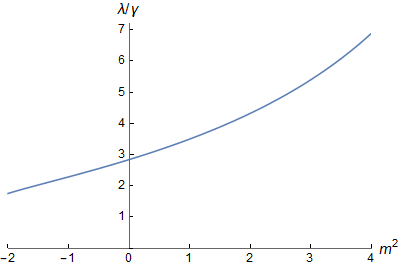
As usual in FPU-like situations, it is natural to expect that the near-perfect returns arise due to proximity to another dynamical system for which the returns are exact. One could first try to improve the quality of returns by variation of parameters of the model, such as the dimension of AdS or the mass of the scalar field. We have explored this scenario in the context of our analytic treatment of solutions dominated by mode 1 in section 4.2. We have seen that by adjusting the mass of the scalar field, it is possible to make the return of mode 3 exact (fig. 8). This evidently qualitatively improves the precision of returns for initial data near mode 1, as the discrepancy is now in the strongly suppressed modes starting from mode 4, but the scenario still falls short of providing exact returns. We also note that a nonrelativistic version of the AdS dynamics (which technically corresponds to the limit of infinite scalar field mass) can be analytically proved to display perfect returns [32] in AdS5, rather than in AdS4 (returns in AdS5 at finite masses, on the other hand, are not close to being perfect).
More broadly, one could look for arbitrary small modifications of the interaction coefficients in (13), irrespectively of whether they originate from standard physically motivated PDEs, and perfect returns in any such system would be sufficient to clarify the origin of near-perfect returns in the (physically motivated) resonant system (13). In [31], a very large class of resonant systems displaying perfect returns for two-mode initial data has been constructed. This class is characterized, in particular, by the following identities satisfied by the interaction coefficients:
| (51) | ||||
where can be either or , and , , , are arbitrary constants. Our numerical comparisons indicate that the interaction coefficients of the resonant system (13) do not appear close to satisfying such relations. One could look for modifications of (51) approximately satisfied by the AdS4 interaction coefficients. Our preliminary study shows that some polynomial-type summation identities are satisfied with a good precision, but we feel that it is premature to judge what exact dynamical implications follow from such approximate identities.
We comment explicitly on what we have achieved in comparison to [8], where the topic of FPU-like behaviors in weakly nonlinear AdS4 dynamics was first brought up. In [8], the focus was on reporting, among other things, the return after three direct-reverse cascades for two-mode initial data with equal energies that can be seen in our fig. 2(d). Since the simulations were performed with a rather limited precision, the results were in principle consistent with perfect returns upset exclusively by numerical artifacts, especially in light of the subsequent discovery of closely related systems for which the returns are exact. We have now ruled out this possibility. At the same time, we have observed imperfect returns of precision much higher than what is suggested by the material of [8] and repeating over many oscillation cycles, as seen in fig. 1. More importantly, our analytic investigations of section 4 have generated a neat picture of returning behaviors for initial data sufficiently close to mode 0 or mode 1, and allowed for identification of specific multiple oscillation periods after which enhanced returns occur. This picture remains valid even for initial data with moderate energy ratios of the two lowest modes. The rational relations between the AdS4 interaction coefficients we have displayed allude to hierarchies of returns, with specific longer waiting times resulting in returns of better and better accuracy. One in fact sees returns of striking accuracy at late times in fig. 6(c), outside the domain where our concrete analytic approximation are valid. This suggests that there are further structures to be explored. Elaborate patterns of returns of varying precision over long times are known from the original FPU problem. (The FPU chain is now believed to thermalize over very long times [39], but in our resonant system (13), the recurrences are likely to persist forever.)
The AdS/CFT paradigm provides an intriguing potential link between our results and dynamics of conformal field theories (CFTs) on spatial spheres. In particular, one would expect that very close returns to the initial state must occur at low energies in CFTs that can be accurately approximated in an appropriate ‘holographic’ limit by a single scalar field in the AdS bulk coupled to gravity. It would be very interesting to delineate this class of systems more precisely, and build explicit connections to the sort of dynamics we have described in this article. There is recent literature [40, 41] providing detailed links between evolution of CFT states and weakly nonlinear gravitational dynamics in the bulk, which is likely to be useful in this regard.
Acknowledgments
We thank Piotr Bizoń and Javier Mas for discussions and for collaboration on related subjects. This research has been supported by CUniverse research promotion project (CUAASC), by FWO-Vlaanderen (projects G044016N and G006918N), by Vrije Universiteit Brussel through the Strategic Research Program “High-Energy Physics,” by FPA2014-52218-P from Ministerio de Economia y Competitividad, by Xunta de Galicia ED431C 2017/07, by the European Regional Development Fund (FEDER) and by Grant María de Maeztu Unit of Excellence MDM-2016-0692. This research has benefited from the use computational resources/services provided by the Galician Supercomputing Centre (CESGA). A.B. thanks the Spanish program “ayudas para contratos predoctorales para la formación de doctores 2015” and its mobility program for his stay at Vrije Universiteit Brussel, where part of this project was developed.
Appendix: Interaction coefficients for a massive scalar field in
We shall consider a massive scalar field in with Dirichlet boundary conditions , which made an appearance in section 5. This model is also fully resonant and an approximation of the form (13) can be derived. The massless case was developed in [9]; the process is quite similar for the massive scalar, so we will only present the main results.
The model is governed by the action
| (52) |
Our ansatz for the metric is (4), with the same conventions as in section 2. Developing the time-averaging strategy described in the main text, or in [9, 10] which contain a more thorough discussion, we obtain the following expressions for the interaction coefficients, after splitting them in three types according to the number of coincident indices, , for and for :
| (53) | ||||
| (54) | ||||
| (55) |
where
| (56) | ||||
| (57) | ||||
| (58) | ||||
| (59) | ||||
| (60) | ||||
| (61) |
Here, and are the eigenmodes and their associated eigenvalues of the linear problem:
| (62) |
Their expressions are
| (63) |
and
| (64) |
where satisfies the equation and are Jacobi polynomials. We have defined and as in (5).
In analogy with the explanation for the massless scalar field given in section 2, the current model has the resonant condition , which through (64) is equivalent to . However there could be two more resonant channels, and , equivalent to and , respectively. If is integer these last two conditions can be satisfied and a priori two new terms must be included in the system of equations (13):
| (65) |
In our situation we did not perform an analytic study of and as in [10], where it was proven that for a massless scalar field () these coefficients vanish, but numerical calculations suggest that they also vanish for nonzero masses. On the other hand, when is not integer, the conditions and are not satisfied for any combination of the indices. Therefore, these interaction channels disappear upon time-averaging. We thus see that, for any , the relevant dynamics is governed by equation (13) through , and .
We note that the given expressions for , and are exactly the same as in [10], where all derivations are specialized to . However, if we were to transform these integrals using integration by parts to the form of [9], the resulting expressions would have differed from those of [9] by additional terms with explicit dependence on .
References
- [1] P. Bizoń and A. Rostworowski, On weakly turbulent instability of anti-de Sitter space, Phys. Rev. Lett. 107 (2011) 031102 arXiv:1104.3702 [gr-qc].
- [2] M. Maliborski and A. Rostworowski, Time-periodic solutions in an Einstein AdS–massless-scalar-field system, Phys. Rev. Lett. 111 (2013) 051102 arXiv:1303.3186 [gr-qc].
- [3] A. Buchel, S. L. Liebling and L. Lehner, Boson stars in AdS spacetime, Phys. Rev. D 87 (2013) 123006 arXiv:1304.4166 [gr-qc].
- [4]
M. Maliborski and A. Rostworowski,
A comment on “Boson stars in AdS,”
arXiv:1307.2875 [gr-qc]. - [5] F. V. Dimitrakopoulos, B. Freivogel, M. Lippert and I. S. Yang, Position space analysis of the AdS (in)stability problem, JHEP 1508 (2015) 077 arXiv:1410.1880 [hep-th].
- [6] N. Kim, Time-periodic solutions of massive scalar fields in dynamical AdS background: perturbative constructions, Phys. Lett. B 742 (2015) 274 arXiv:1411.1633 [hep-th].
- [7] N. Deppe and A. R. Frey, Classes of stable initial data for massless and massive scalars in Anti-de Sitter spacetime, JHEP 1512, 004 (2015) arXiv:1508.02709 [hep-th].
- [8] V. Balasubramanian, A. Buchel, S. R. Green, L. Lehner and S. L. Liebling, Holographic thermalization, stability of anti-de Sitter space, and the Fermi-Pasta-Ulam paradox, Phys. Rev. Lett. 113 (2014) 071601 arXiv:1403.6471 [hep-th].
- [9] B. Craps, O. Evnin and J. Vanhoof, Renormalization group, secular term resummation and AdS (in)stability, JHEP 1410 (2014) 48 arXiv:1407.6273 [gr-qc].
- [10] B. Craps, O. Evnin and J. Vanhoof, Renormalization, averaging, conservation laws and AdS (in)stability, JHEP 1501 (2015) 108 arXiv:1412.3249 [gr-qc].
- [11] I-S. Yang, Missing top of the AdS resonance structure, Phys. Rev. D 91 (2015) 065011 arXiv:1501.00998 [hep-th].
- [12] O. Evnin and R. Nivesvivat, AdS perturbations, isometries, selection rules and the Higgs oscillator, JHEP 1601 (2016) 151 arXiv:1512.00349 [hep-th].
- [13] P. Basu, C. Krishnan and A. Saurabh, A stochasticity threshold in holography and the instability of AdS, Int. J. Mod. Phys. A 30 (2015) 1550128 arXiv:1408.0624 [hep-th].
- [14] A. Buchel, S. R. Green, L. Lehner and S. L. Liebling, Conserved quantities and dual turbulent cascades in anti-de Sitter spacetime, Phys. Rev. D 91 (2015) 064026 arXiv:1412.4761 [gr-qc].
- [15] P. Bizoń, M. Maliborski, A. Rostworowski, Resonant dynamics and the instability of anti-de Sitter spacetime, Phys. Rev. Lett. 115 (2015) 081103 arXiv:1506.03519 [gr-qc].
- [16] B. Craps and O. Evnin, AdS (in)stability: an analytic approach, Fortsch. Phys. 64 (2016) 336 arXiv:1510.07836 [gr-qc].
- [17] P. Bizoń and A. Rostworowski, Gravitational turbulent instability of AdS5, Acta Phys. Polon. B 48 (2017) 1375 arXiv:1710.03438 [gr-qc].
- [18] O. J. C. Dias, G. T. Horowitz and J. E. Santos, Gravitational turbulent instability of Anti-de Sitter space, Class. Quant. Grav. 29 (2012) 194002 arXiv:1109.1825 [hep-th].
- [19] E. Fermi, J. Pasta, and S. Ulam, Studies of the nonlinear problems I, Los Alamos Report LA-1940, (1955), reprinted in Collected Papers of Enrico Fermi, ed. E. Segre, Vol. II (University of Chicago Press, 1965).
- [20] G. P. Berman and F. M. Izrailev, The Fermi-Pasta-Ulam problem: 50 years of progress, Chaos 15 (2005) 015104 arXiv:nlin/0411062.
- [21] P. Bizoń, B. Craps, O. Evnin, D. Hunik, V. Luyten and M. Maliborski, Conformal flow on and weak field integrability in AdS4, Comm. Math. Phys. 353 (2017) 1179 arXiv:1608.07227 [math.AP].
- [22] P. Bizoń, D. Hunik-Kostyra and D. Pelinovsky, Ground state of the conformal flow on , arXiv:1706.07726 [math.AP].
- [23] B. Craps, O. Evnin and V. Luyten, Maximally rotating waves in AdS and on spheres, JHEP 1709 (2017) 059 arXiv:1707.08501 [hep-th].
- [24] P. Bizoń, D. Hunik-Kostyra and D. E. Pelinovsky, Stationary states of the cubic conformal flow on , arXiv:1807.00426 [math-ph].
- [25] P. Germain, Z. Hani and L. Thomann, On the continuous resonant equation for NLS: I. Deterministic analysis, J. Math. Pur. App. 105 (2016) 131 arXiv:1501.03760 [math.AP].
- [26] P. Germain and L. Thomann, On the high frequency limit of the LLL equation, Quart. Appl. Math. 74 (2016) 633 arXiv:1509.09080 [math.AP].
- [27] A. F. Biasi, J. Mas and A. Paredes, Delayed collapses of BECs in relation to AdS gravity, Phys. Rev. E 95 (2017) 032216 arXiv:1610.04866 [nlin.PS].
- [28] A. Biasi, P. Bizoń, B. Craps and O. Evnin, Exact lowest-Landau-level solutions for vortex precession in Bose-Einstein condensates, Phys. Rev. A 96 (2017) 053615 arXiv:1705.00867 [cond-mat.quant-gas].
- [29] P. Gérard, P. Germain and L. Thomann, On the cubic lowest Landau level equation, arXiv:1709.04276 [math.AP].
- [30] A. Biasi, P. Bizoń, B. Craps and O. Evnin, Two infinite families of resonant solutions for the Gross-Pitaevskii equation, Phys. Rev. E 98 (2018) 032222 arXiv:1805.01775 [cond-mat.quant-gas].
- [31] A. Biasi, P. Bizoń and O. Evnin, Solvable cubic resonant systems, arXiv:1805.03634 [nlin.SI].
- [32] P. Bizoń, O. Evnin and F. Ficek, A non-relativistic limit for AdS perturbations, arXiv:1810.10574 [gr-qc].
- [33] C. Sulem, P.-L. Sulem and H. Frisch, Tracing complex singularities with spectral methods, J. Comput. Phys. 50 (1983) 138.
- [34] P. Bizoń and J. Jałmużna, Globally regular instability of , Phys. Rev. Lett. 111 (2013) no.4, 041102 arXiv:1306.0317 [gr-qc].
- [35] B. Craps, O. Evnin, P. Jai-akson and J. Vanhoof, Ultraviolet asymptotics for quasiperiodic AdS4 perturbations, JHEP 1510 (2015) 080 arXiv:1508.05474 [gr-qc].
- [36] S. R. Green, A. Maillard, L. Lehner and S. L. Liebling, Islands of stability and recurrence times in AdS, Phys. Rev. D 92 (2015) 084001 arXiv:1507.08261 [gr-qc].
- [37] O. Evnin and C. Krishnan, A hidden symmetry of AdS resonances, Phys. Rev. D 91 (2015) 126010 arXiv:1502.03749 [hep-th].
- [38] O. Evnin, H. Demirchian and A. Nersessian, Klein-Gordonization: mapping superintegrable quantum mechanics to resonant spacetimes, Phys. Rev. D 97 (2018) 025014 arXiv:1711.03297 [hep-th].
- [39] M. Onorato, L. Vozella, D. Proment and Y. V. Lvov, Route to thermalization in the -Fermi-Pasta-Ulam system, PNAS 112 (2015) 4208 arXiv:1402.1603 [nlin.CD].
- [40] T. Faulkner, F. M. Haehl, E. Hijano, O. Parrikar, C. Rabideau and M. Van Raamsdonk, Nonlinear gravity from entanglement in conformal field theories, JHEP 1708 (2017) 057 arXiv:1705.03026 [hep-th].
- [41] E. Oh, I. Y. Park and S. J. Sin, Complete Einstein equations from the generalized first law of entanglement, Phys. Rev. D 98 (2018) 026020 arXiv:1709.05752 [hep-th].