Pluripotential theory on Teichmüller space II
– Poisson integral formula –Thanks: t This work is partially supported by JSPS KAKENHI Grant Numbers 20H01800, 20K20519, 18KK0071, and was partially supported by JSPS KAKENHI Grant Numbers 16K05202, 16H03933, 17H02843

Hideki Miyachi Address: School of Mathematics and Physics, College of Science and Engineering, Kanazawa University, Kakuma-machi, Kanazawa, Ishikawa, 920-1192, Japan Email address: miyachi@se.kanazawa-u.ac.jp

Date: August 11, 2026

Abstract.

This is the second paper in a series of investigations of the pluripotential theory on Teichmüller space. The main purpose of this paper is to establish the Poisson integral formula for pluriharmonic functions on Teichmüller space which are continuous on the Bers compactification. We also observe that the Schwarz type theorem on the boundary behavior of the Poisson integral. We will see a relationship between the pluriharmonic measures and the Patterson-Sullivan measures discussed by Athreya, Bufetov, Eskin and Mirzakhani.

Key words and phrases:

Singular Euclidean structures, Teichmüller space, Teichmüller distance, Levi forms, Pluricomplex Green functions, Poisson integral formula, Thurston measure

2010 Mathematics Subject Classification

32G05, 32G15, 32U15, 32U35, 57M50, 26B20, 30E20

1. Introduction

This is the second paper in a series of investigations of the pluripotential theory on Teichmüller space. The first paper in the series is [71] in which we discussed an alternative approach to the Krushkal formula ([50]) of the pluricomplex Green function on the Teichmüller space (cf. (10.21)). The main purpose of this paper is to establish the Poisson integral formula for pluriharmonic functions on Teichmüller space which are continuous on the Bers compactification. This result is announced in [72] and [73].

1.1. Classical Poisson integral formula and a dictionary

It is well-known that any continuous function $u$ on the closed upper half-plane $\overline{\mathbb{H}}=\mathbb{H}\cup(\mathbb{R}\cup\{\infty\})$ which is harmonic on the upper-half plane $\mathbb{H}$ satisifies

(1.1)

u(z)=\int_{\partial\mathbb{H}}P(z,\xi)u(\xi)\dfrac{d\xi}{\pi},

for $z=x+iy\in\mathbb{H}$ , where $\partial\mathbb{H}=\mathbb{R}\cup\{\infty\}$ and

P(z,\xi)=\dfrac{{\rm Im}(z)}{|z-\xi|^{2}}.

The integral representation (1.1) is called the Poisson integral formula. Meanwhile, it is also well-known that the Teichmüller space $\mathcal{T}_{1}$ of tori is identified with the upper-half plane $\mathbb{H}$ via the period map. In recognizing the Poisson integral formula (1.1) as the formula for the (pluri)harmonic functions on the Teichmüller space $\mathcal{T}_{1}$ , we obtain a dictionary as Table 1 in the case of tori (i,e, $(g,m)=(1,0)$ ) (cf. §2.1). In this paper, we will justify the correspondence in Table 1 for arbitrary $(g,m)$ , as we state in Theorem 1.1.

Upper half-plane

\mathbb{H}

Teichmüller space

\mathcal{T}_{g,m}

Harmonic function

Pluriharmonic function

Ideal boundary

\partial\mathbb{H}

Bers boundary

Green function

\log\tanh

of the Teichmüller distance

Horofunctions (Busemann functions)

log of extremal lengths

Poisson kernel

Ratio of extremal lengths

Harmonic measure on

\partial\mathbb{H}

Pushforward measure of

the normalized Thurston measure

Table 1. A dictionary

1.2. Results

Let $\mathcal{T}_{g,m}$ be the Teichmüller space of type $(g,m)$ . Let $\mathcal{T}^{B}_{x_{0}}$ be the Bers slice with base point $x_{0}\in\mathcal{T}_{g,m}$ . Krushkal [49] showed that Teichmüller space is hyperconvex. By the Nehari-Kraus theorem, the Bers slice $\mathcal{T}^{B}_{x_{0}}$ is a bounded domain in a finite dimensional complex Banach space (cf. [6]). Demailly [21] establishes fundamental results in the pluripotential theory, the existence of the pluricomplex Green functions and the pluriharmonic measures for bounded hyperconvex domains in the complex Euclidean space (see §9).

1.2.1. Results

Let $\partial\mathcal{T}^{B}_{x_{0}}$ be the Bers boundary of $\mathcal{T}^{B}_{x_{0}}\cong\mathcal{T}_{g,m}$ and $\partial^{ue}\mathcal{T}^{B}_{x_{0}}$ the subset of $\partial\mathcal{T}^{B}_{x_{0}}$ which consists of totally degenerate groups without APT whose ending laminations are the supports of minimal, filling and uniquely ergodic measured laminations. We define a function $\mathbb{P}$ on $\mathcal{T}_{g,m}\times\mathcal{T}_{g,m}\times\partial\mathcal{T}^{B}_{x_{0}}$ by

(1.2)

\mathbb{P}(x,y,\varphi)=\begin{cases}{\displaystyle\left(\frac{{\rm Ext}_{x}(F_{\varphi})}{{\rm Ext}_{y}(F_{\varphi})}\right)^{3g-3+m}}&(\varphi\in\partial^{ue}\mathcal{T}^{B}_{x_{0}}),\\ 1&(\mbox{otherwise}),\end{cases}

where for $\varphi\in\partial^{ue}\mathcal{T}^{B}_{x_{0}}$ , $F_{\varphi}$ is the measured foliation corresponding to the measured lamination whose support is the ending lamination of the Kleinian manifold associated to $\varphi$ , and ${\rm Ext}_{x}(F)$ is the extremal length of a measured foliation $F$ on $x\in\mathcal{T}_{g,m}$ (cf. §4.2).

The main result of this paper is as follows.

Theorem 1.1 (Poisson integral formula).

Let $V$ be a continuous function on the Bers compactification $\overline{\mathcal{T}^{B}_{x_{0}}}$ which is pluriharmonic on $\mathcal{T}^{B}_{x_{0}}\cong\mathcal{T}_{g,m}$ . Then

(1.3)

V(x)=\int_{\partial\mathcal{T}^{B}_{x_{0}}}V(\varphi)\mathbb{P}(x_{0},x,\varphi)d{\boldsymbol{\mu}}^{B}_{x_{0}}(\varphi),

where ${\boldsymbol{\mu}}^{B}_{x_{0}}$ is the probability measure on $\partial\mathcal{T}^{B}_{x_{0}}$ defined as the pushforward measure of the Thurston measure on the space $\mathcal{PMF}$ of projective measured foliations associated with $x_{0}$ . Especially, the function (1.2) is the Poisson kernel for pluriharmonic functions on Teichmüller space.

See §6 for the precise definition of the probability measure ${\boldsymbol{\mu}}^{B}_{x_{0}}$ on $\partial\mathcal{T}^{B}_{x_{0}}$ . Theorem 1.1 follows from the Green formula for plurisubharmonic functions stated in Theorem 13.1. We see that the measure $d{\boldsymbol{\mu}}^{B}_{x}=\mathbb{P}(x_{0},x,\cdot)d{\boldsymbol{\mu}}^{B}_{x_{0}}$ coincides with Demailly’s pluriharmonic measure of $x\in\mathcal{T}_{g,m}$ (cf. Theorem 13.2). The formula (1.3) is rephrased as the integrable representation of integral functions on $\mathcal{PMF}$ (cf. §15.1).

Following [4, §2.3.1], we define the cocycle function by

\beta(x,y,\varphi)=\begin{cases}{\displaystyle\frac{1}{2}(\log{\rm Ext}_{x}(F_{\varphi})-\log{\rm Ext}_{y}(F_{\varphi}))}&(\varphi\in\partial^{ue}\mathcal{T}^{B}_{x_{0}}),\\[5.69054pt] 0&(\mbox{otherwise})\end{cases}

for $(x,y,\varphi)\in\mathcal{T}_{g,m}\times\mathcal{T}_{g,m}\times\partial\mathcal{T}^{B}_{x_{0}}$ . The cocycle function $\beta$ is also understood as the horofunction for the Teichmüller distance when $\varphi\in\partial^{ue}\mathcal{T}^{B}_{x_{0}}$ (cf. [54]. See also [67] and [68]). The Poisson integral formula (1.3) is rewritten as

(1.4)

V(x)=\int_{\partial\mathcal{T}^{B}_{x_{0}}}V(\varphi)e^{-(6g-6+2m)\beta(x,x_{0},\varphi)}d{\boldsymbol{\mu}}^{B}_{x_{0}}(\varphi).

The formulation (1.4) implies that Demailly’s pluriharmonic measures $\{{\boldsymbol{\mu}}^{B}_{x}\}_{x\in\mathcal{T}_{g,m}}$ are thought of as the conformal density of dimension $6g-6+2m$ on $\partial\mathcal{T}^{B}_{x_{0}}$ (cf. [4, §2.3.1] and [36]. See also Remark 15.1). This observation is in complete analogy with that in the case of the hyperbolic spaces (cf. §2.1 See also [72] and [63, Theorem B]).

In the proof of Theorem 1.1, we realize Teichmüller space as a convex cone in the $6g-6+2m$ dimensional Euclidean space (cf. §8). We give an explicit presentation of the complex structure on the convex cone which makes the realization biholomorphic (cf. (8.11) and Proposition 8.3). The $\partial$ and $\overline{\partial}$ -derivatives and the Levi form of extremal lengths in Proposition 10.1 are calculated with this complex structure (cf. [74]). An advantage of this realization is that the Monge-Ampère measure of the extremal length function is simply represented (cf. (10.7)). Riera [83] described the complex structure on Teichmüller space in terms of the Fenchel-Nielsen coordinates. Our presentation is thought of as a counterpart of Riera’s one.

Schwarz [85] studied the behavior of the Poisson integral of integrable functions on the unit circle around points where given functions are continuous (see also [90, Theorem IV.2]). We will observe an analogy with Schwarz’s theorem as follows (cf. §14).

Theorem 1.2 (Schwarz type theorem).

Let $V$ be an integrable function on $\partial\mathcal{T}^{B}_{x_{0}}$ with respect to ${\boldsymbol{\mu}}^{B}_{x_{0}}$ . When $V$ is continuous at $\varphi_{0}\in\partial^{ue}\mathcal{T}^{B}_{x_{0}}$ ,

\lim_{\mathcal{T}_{g,m}\ni x\to\varphi_{0}}\int_{\partial\mathcal{T}^{B}_{x_{0}}}V(\varphi)\mathbb{P}(x_{0},x,\varphi)d{\boldsymbol{\mu}}^{B}_{x_{0}}(\varphi)=V(\varphi_{0}).

As a corollary, we deduce

Corollary 1.1 (Holomorphic extension).

Let $V$ be a complex-valued integrable function on $\partial\mathcal{T}^{B}_{x_{0}}$ with respect to ${\boldsymbol{\mu}}^{B}_{x_{0}}$ . Suppose that $V$ is continuous on $\partial^{ue}\mathcal{T}^{B}_{x_{0}}$ . If

(1.5)

\int_{\partial\mathcal{T}^{B}_{x_{0}}}V(\varphi)\overline{\partial}\mathbb{P}(x_{0},\,\cdot\,,\varphi)d{\boldsymbol{\mu}}^{B}_{x_{0}}(\varphi)=0

on $\mathcal{T}_{g,m}$ as $(0,1)$ -forms, then the Poisson integral

P[V](x)=\int_{\partial\mathcal{T}^{B}_{x_{0}}}V(\varphi)\mathbb{P}(x_{0},x,\varphi)d{\boldsymbol{\mu}}^{B}_{x_{0}}(\varphi)

is a holomorphic function on $\mathcal{T}_{g,m}$ and satisfies

\lim_{\mathcal{T}_{g,m}\ni x\to\varphi_{0}}P[V](x)=V(\varphi_{0})\quad(\varphi_{0}\in\partial^{ue}\mathcal{T}^{B}_{x_{0}}).

In the complex function theory on $\mathcal{T}_{g,m}$ , Equation (1.5) will play as the homogeneous tangential Cauchy-Riemann equation (in the distribution sense) for the boundary functions of holomorphic functions on Teichmüller space, which characterizes the boundary functions of holomorphic functions (cf. [13]).

Notice from Theorem 1.1 that continuous functions on $\partial\mathcal{T}^{B}_{x_{0}}$ with holomorphic extensions on $\mathcal{T}_{g,m}$ satisfy (1.5). Unlike in the case of the unit disk, it is not clear whether the Poisson integral

\int_{\partial\mathcal{T}^{B}_{x_{0}}}V(\varphi)\mathbb{P}(x_{0},x,\varphi)d{\boldsymbol{\mu}}^{B}_{x_{0}}(\varphi)

is pluriharmonic on $\mathcal{T}_{g,m}$ for any integrable function $V$ on $\partial\mathcal{T}^{B}_{x_{0}}$ (cf. Remark 12.1).

1.3. Applications

Applying the Poisson integral formula (1.3) to $V\equiv 1$ , we deduce that the Hubbard-Masur function is constant. Namely, the volume of the unit ball in $\mathcal{MF}$ with respect to the extremal length depends only on the topological type of $\Sigma_{g,m}$ (cf. Corollary 15.2). This is first proved by Mirzakhani and Dumas (cf. [24, Theorem 5.10]).

The Poisson integral formula is thought of as a generalization of the mean value theorem. Namely, the value of a (pluri)harmonic function in the domain is the average of the boundary value with harmonic measures. Applying the Poisson integral formula (1.3), we will give the vector-valued (quadratic differential-valued) measures on $\mathcal{PMF}$ which describe the $\partial$ and $\overline{\partial}$ -differentials of pluriharmonic functions on $\mathcal{T}_{g,m}$ which is continuous on the Bers closure (cf. §15.2.1). Applying this description to the trace functions of boundary groups of the Bers slice, we will represent Wolpert’s quadratic differentials $\Theta_{\gamma,x}$ which corresponds to the differentials of the hyperbolic lengths of closed geodesics $\gamma$ in terms of the Hubbard-Masur differentials $q_{F,x}$ ( $F\in\mathcal{MF}$ ) by the averaging procedure as follows.

Theorem 1.3 (Representation of Wolpert’s differentials).

For $x\in\mathcal{T}_{g,m}$ and $\gamma\in\pi_{1}(\Sigma_{g,m})$ , we have

(1.6)

\Theta_{\gamma,x}=\frac{{\boldsymbol{\xi}}}{2\sinh(\ell_{\gamma}(x))}\int_{\mathcal{PMF}^{mf}}{\rm tr}^{2}\left(\rho_{\varphi_{[F],x}}(\gamma)\right)\,\frac{q_{F,x}}{\|q_{F,x}\|}d\hat{\mu}_{Th}^{x}([F]).

The definitions of the symbols in the formula (1.6) and the proof of Theorem 1.3 can be found in §15.2.2. The representation (1.6) gives an interaction between the $L^{2}$ -geometry on Teichmüller space (Weil-Petersson Riemannian-Kählerian geometry) and the $L^{1}$ or $L^{\infty}$ -geometry (Teichmüller Finsler geometry) on Teichmüller space.

1.4. History, Motivation and Future

The complex analytic structure on Teichmüller space was described by Ahlfors with the variational formula of the period matrix (cf. [3]. See also [81]). Bers [6] realized Teichmüller space as a bounded domain, called the Bers slice, in a finite dimensional complex Banach space. Teichmüller space has rich and interesting properties in the complex analytical aspect. For instance, Teichmüller space is Stein (Bers-Ehrenpreis [11]); the holomorphic automorphism group is (essentially) isomorphic to the mapping class group (Royden [84]); the moduli space is Kähler hyperbolic (McMullen [60]); the Kobayashi distance coincides with the Kobayashi distance (Royden [84] and Earle-Kra [27]) but it does not coincide with the Carathéodory distance (Markovic [55]).

A naive problem behind our research

Any holomorphic invariant of (marked) Riemann surfaces or Kleinian groups is thought of as a holomorphic function on Teichmüller space, and the algebra of holomorphic functions characterizes Teichmüller space as a complex manifold up to complex conjugation (cf. [41]). A fundamental problem behind this research is:

Problem 1.

What are reasonable geometric objects which represent holomorphic functions on Teichmüller spaces?

The Teichmüller space is known to be the universal space of holomorphic families in the sense that holomorphic mappings into Teichmüller space admit geometric interpretations, holomorphic families of Riemann surfaces (cf. [88]. See also [79] for a commentary and an English translation of [88]).

Why Bers slices?

There are many realizations of the Teichmüller space as domains in the Euclidean space which are base points free (e.g. [26], [28], [56]). One may ask why we think the Bers slice.

The Bers slice is mysterious: The Bers slice is defined by a transcendental manner, and is deeply related to the theory of univalent functions (cf.§5.2). The Bers slices depend the base point (cf. [43]). The Bers boundary is conjectured to be fractal and self-similar at the fixed point with respect to the pseudo-Anosov mapping class action (See Figure 1. See [19], [48] and [59, Problem 7 in Chapter 10]). To approach these conjectures, it seems necessary to understand a detailed relation between the holomorphic (geometric) structure and the topological aspect of the Teichmüller theory around the boundary. Despite such interesting problems are posed, to the author’s knowledge, there is less mathematical tools for investigating the holomorphic structure around the Bers boundary, and it is expected to develop the complex analytical aspect of the Teichmüller theory to clarify the relation. Actually, Problem 1 is motivated from these conjectures.

Refer to caption — Figure 1. The Bers slice of once punctured tori whose base point is the square torus. Courtesy of Professor Yasushi Yamashita (cf. [48]).

The Bers slice is itself an interesting bounded domain in view of Complex analysis: It is hyperconvex (Krushkal [49]), and its closure is polynomially convex (Shiga [86], Deroin-Dujardan [22]). Indeed, due to the polynomially convexity, almost all of holomorphic functions on $\mathcal{T}_{g,m}$ are represented by the Poisson integral formula (1.3) in the sense that any holomorphic function on $\mathcal{T}_{g,m}$ is approximated by holomorphic functions on the ambient space of the Bers slice.

Complex analysis encounters the Thurston theory

In a celebrated paper [18], Brock, Canary and Minsky settled the ending lamination theorem. The ending lamination theorem enables us to parametrize the Bers boundary by topological invariants called the end-invariants, and makes a strong connection between the complex analytical aspect in Teichmüller theory and the Thurston theory (the topological aspect in Teichmüller theory) (cf. §5). Our research is based on sophisticated results in the theory of Kleinian groups as well as Teichmüller theory.

To approach Problem 1, we attempt to realize holomorphic functions as functions on spaces coming out from the topological aspect. The Bers boundary and the space of projective measured foliations are thought of as being essentially assembled from topological invariants by the ending lamination theorem.

The extremal length functions, which appear in the Poisson kernel (1.2), are thought of as the intersection number between marked Riemann surfaces and measured foliations in Extremal length geometry (cf. [62, Lemma 5.1], [32], [68] and §4.3). Thus, the Poisson integral formula (1.3) and the homogeneous Cauchy-Riemann equation (1.5) are expected to strengthen the connection between the complex-analytical aspect and the topological aspect in Teichmüller theory, and to develop Complex analysis on Teichmüller space with Thurston theory.

1.5. About this paper

This paper is organized as follows. In §2, we discuss the case of tori for a model case of our main theorem. From §3 to §6, we recall basics and known results in Teichmüller theory. In §8 and §10, we recall and discuss the holomorphic coordinates associated to the extremal length functions of essentially complete measured foliations developed in [74], and the presentation of the Levi forms of the extremal length functions.

The proof of Theorem 1.1 is accomplished in the discussion from §11 to §13. In the proof, we will compare the Thurston measure on the unit sphere in $\mathcal{MF}$ in terms of extremal length functions with the measures defined on the pluricomplex Green function on the level set (cf. Proposition 11.2). For the comparison, we adopt the reciprocals of extremal length functions as mediators (cf. (10.25)). We will prove Theorem 1.2 in §14.

§15, we rephrase the integral representation (1.3) in terms of the integration on $\mathcal{PMF}$ and discuss the integral representation of the $\partial$ and $\overline{\partial}$ -differentials of pluriharmonic functions on $\mathcal{T}_{g,m}$ (cf. Corollary 15.1 and (15.3)). The holomorphic quadratic differentials associated to the differentials of hyperbolic lengths of closed geodesics are represented by averaging the Hubbard-Masur differentials by the Thurston measure (cf. (15.6) and Theorem 1.3).

Acknowledgement

The author would like to express his gratitude to anonymous referees for valuable comments. He also thanks Professor Ken’ichi Ohshika and Professor Athanase Papadopoulous for their constant encouragements.

2. One dimensional cases

2.1. Case of tori

We check the correspondence in Table 1 for tori. We start with recalling the horofunction compactification of the Teichmüller space of tori. The horofunctions are presented with the extremal length. We will see the same conclusion holds for arbitrary $(g,m)$ in §4.

Let $\Sigma_{1}$ be a (topolotical) torus and $A$ and $B$ are generators of the fundmanetal group $\pi_{1}(\Sigma_{1})\cong H_{1}(\Sigma_{1})$ such that the algebraic intersection number $A\cdot B$ is $+1$ . As discussed above, the Teichmüller space $\mathcal{T}_{1}$ is identified with $\mathbb{H}$ in the sense that any marked torus is biholomorphically equivalent to $X_{\tau}=\mathbb{C}/\Gamma_{\tau}$ where $\Gamma_{\tau}$ is the lattice on $\mathbb{C}$ generated by $1$ and $\tau\in\mathbb{H}$ and the marking $\Sigma_{1}\to X_{\tau}$ sends $A$ to $1$ and $B$ to $\tau$ . We denote by $x_{\tau}\in\mathcal{T}_{1}$ the marked tori associated to $\tau\in\mathbb{H}$ .

The free homotopy classes of simple closed curves on a (topological) torus $\Sigma_{1}$ is enumerated by $\hat{\mathbb{Q}}=\mathbb{Q}\cup\{\infty\}$ ( $\infty=\pm 1/0$ ). In our convention, the $p/q$ -curve on $\Sigma_{1}$ corresponds to $-pA+qB$ , where $p$ and $q$ are taken to be relatively prime when $pq\neq 0$ , $p=1$ when $q=0$ , and $q=1$ when $p=0$ . The space of measured foliation $\mathcal{MF}(\Sigma_{1})$ on $\Sigma_{1}$ is canonically identified with the quotient space $\mathbb{R}^{2}/(x,y)\sim(-x,-y)$ , so that the $p/q$ -curve corresponds to the equivalence class $[-p,q]\in\mathbb{R}^{2}/(x,y)\sim(-x,-y)$ of $(-p,q)\in\mathbb{R}^{2}$ . The space $\mathcal{PMF}(\Sigma_{1})=(\mathcal{MF}(\Sigma_{1})-\{0\})/\mathbb{R}_{>0}$ of projective measured foliations is identified with $\partial\mathbb{H}=\hat{\mathbb{R}}=\mathbb{R}\cup\{\infty\}$ , and the identification is induced by the map

(2.1)

\Pi_{1}\colon\mathcal{MF}(\Sigma_{1})=\mathbb{R}^{2}/(x,y)\sim(-x,-y)\ni[a,b]\mapsto-a/b\in\hat{\mathbb{R}}.

The extremal length ${\rm Ext}_{\tau}(F_{[}a,b])$ of the measured foliation $F_{[a,b]}$ is equal to

{\rm Ext}_{\tau}([a,b])=\dfrac{|a+b\tau|^{2}}{{\rm Im}(\tau)}.

The Teichmüller distance on $\mathcal{T}_{1}$ coincides with the hyperbolic distance $d_{\mathbb{H}}$ of curvature $-4$ , and Kerckhoff’s formula holds:

d_{T}(x_{\tau_{1}},x_{\tau_{2}})=\dfrac{1}{2}\log\sup_{p/q\in\hat{\mathcal{Q}}}\dfrac{{\rm Ext}_{x_{\tau_{1}}}(C_{p/q})}{{\rm Ext}_{x_{\tau_{2}}}(C_{p/q})}=\dfrac{1}{2}\log\dfrac{|\tau_{1}-\overline{\tau_{2}}|+|\tau_{1}-\tau_{2}|}{|\tau_{1}-\overline{\tau_{2}}|-|\tau_{1}-\tau_{2}|}.

The horofunction appears in the horofunction compactification (introduced by Gromov [34]) which is defined by the closure of the embedding (defined with basepoint $\tau=\tau_{0}$ )

\mathcal{T}_{1}\ni x_{\tau_{1}}\mapsto[\mathcal{T}_{1}\ni\tau\mapsto d_{T}(x_{\tau},x_{\tau_{1}})-d_{T}(x_{\tau_{1}},x_{\tau_{0}})]\in C^{0}(\mathcal{T}_{1})

into the space of continuous functions on $\mathcal{T}_{1}$ (endowed with the topology of uniform convergence on any compact sets). In the case of $(\mathcal{T}_{1},d_{T})\cong(\mathbb{H},d_{\mathbb{H}})$ , the horofunction compactification canonically coincides with the closure $\overline{\mathbb{H}}=\mathbb{H}\cup\hat{\mathbb{R}}$ . The horofunction associated to $\Pi_{1}([a,b])=-a/b\in\hat{\mathbb{R}}$ is

	$\displaystyle\mathfrak{h}(x_{\tau},x_{\tau_{0}},-a/b)$	$\displaystyle=\lim_{\tau_{1}\to-a/b}(d_{T}(\tau,x_{\tau_{1}})-d_{T}(x_{\tau_{1}},x_{\tau_{0}}))$
		$\displaystyle=\frac{1}{2}\log\dfrac{{\rm Im}(\tau_{0})}{{\rm Im}(\tau)}\dfrac{\|a+b\tau\|^{2}}{\|a+b\tau_{0}\|^{2}}$
		$\displaystyle=\frac{1}{2}(\log{\rm Ext}_{x_{\tau}}(F_{[a,b]})-\log{\rm Ext}_{x_{\tau_{0}}}(F_{[a,b]})).$

The Thurston measure $\mu_{Th}$ on $\mathcal{MF}(\Sigma_{1})$ is induced by the Euclidean measure on $\mathbb{R}^{2}$ up to multiplying positive constants. The measure $\mu_{Th}$ is a mapping class group-invariant and ergodic measure supported on the filling measured foliations (e.g. [37] and [51]. See also [53]). In the case of tori, filling measured foliations correspond to points in $\mathcal{MF}(\Sigma_{1})=\mathbb{R}^{2}/(x,y)\sim(-x,-y)$ with irrational slopes. Let $F_{[a,b]}$ be the measured foliation labeled $[a,b]\in\mathcal{MF}(\Sigma_{1})$ . The unit sphere in terms of the extremal length function $\mathcal{SMF}_{x_{\tau}}=\{F\in\mathcal{MF}\mid{\rm Ext}_{x_{\tau}}(F)=1\}$ is (the quotient of) an ellipse $\{[a,b]\mid|a+b\tau|^{2}={\rm Im}(\tau)\}$ . The (normalized) Thurston measure $\hat{\mu}_{Th}^{\tau}$ associated to $\tau\in\mathbb{H}\cong\mathcal{T}_{1}$ is a Borel measure on the ellipse $\mathcal{SMF}_{x_{\tau}}$ , which is defined by the cone extension (cf. (6.3)). The pushforward measure ${\boldsymbol{\mu}}_{\tau}=(\Pi_{1})_{*}(\hat{\mu}_{Th}^{\tau})$ on $\hat{\mathbb{R}}=\partial\mathbb{H}=\partial\mathcal{T}_{1}$ is

(2.2)

{\boldsymbol{\mu}}_{\tau}(A)=\int_{A}\dfrac{{\rm Im}(\tau)}{|\tau-\xi|^{2}}\dfrac{d\xi}{\pi}

for $A\subset\hat{\mathbb{R}}$ , which is nothing but the harmonic measure on $\mathbb{H}$ at $\tau$ (cf. [33, §I.1]). The unit sphere $\mathcal{SMF}_{x_{\tau}}$ is thought of as the infinitesimal circle in the tangent space and the harmonic measure (the pushforward measure) is the visual angle measure (e.g. [33, §1]). Thus, the classical Poisson integral formula (1.1) is written as

u(\tau)=\int_{\partial\mathcal{T}_{1}}u(\xi)e^{-2\mathfrak{h}(x_{\tau},x_{\tau_{0}},\xi)}d{\boldsymbol{\mu}}_{\tau_{0}}(\xi)

with fixed $\tau_{0}\in\mathcal{T}_{1}$ , as discussed around (1.4).

2.2. Cases of once punctured tori and fourth punctured spheres

The Teichmüller space $\mathcal{T}_{1,1}$ of once punctured tori is canonically identified with the Teichmüller space $\mathcal{T}_{1}$ of tori and hence with the upper-half plane $\mathbb{H}$ . Hence we write $x_{\tau}$ a point in $\mathcal{T}_{1,1}$ corresponding to $\tau\in\mathbb{H}$ as §2.1. From the commensurability, the Bers embedded the Teichmüller space $\mathcal{T}_{0,4}$ of fourth punctured spheres canonically coincides with that of $\mathcal{T}_{1,1}$ (cf. [47, Lemma 3.1]).

Fix $x_{0}\in\mathcal{T}_{1,1}$ . Let $\mathcal{T}^{B}_{x_{0}}$ be the Bers slice of once punctured tori with base point $x_{0}$ (cf. §5.2. See also Figure 1). The identification $\mathbb{H}\cong\mathcal{T}^{B}_{x_{0}}$ is nothing but the Riemann mapping. Since the Bers slice is a Jordan domain, the identification extends the closures $\overline{\mathbb{H}}\to\overline{\mathcal{T}^{B}_{x_{0}}}$ (cf. [63]). The map $\partial\mathbb{H}\to\partial\mathcal{T}^{B}_{x_{0}}$ induced from the Riemann mapping coinsides with the mapping defined from the ending lamination theorem after identifying $\partial\mathbb{H}\cong\mathcal{PMF}$ by (2.1).

The harmonic measure ${\boldsymbol{\mu}}^{B}_{x_{\tau}}$ at $x_{\tau}\in\mathcal{T}_{1,1}\cong\mathcal{T}^{B}_{x_{0}}$ on the Bers boundary $\partial\mathcal{T}^{B}_{x_{0}}$ is the pushforward measure of (2.2), and hence, the harmonic measure ${\boldsymbol{\mu}}^{B}_{x_{\tau}}$ is the pushforward measure of the normalized Thurston measure $\hat{\mu}_{Th}^{\tau}$ on the unit sphere $\mathcal{SMF}_{x_{\tau}}$ of the extremal length function via $\mathcal{SMF}_{x_{\tau}}\to\partial\mathcal{T}^{B}_{x_{0}}\cong\partial\mathbb{H}$ as discussed in §2.1. Therefore, our main theorem, Theorem 1.3, in this case follows from these observations (cf. [33]).

3. Teichmüller theory

Let $\Sigma_{g,m}$ be a closed orientable surface of genus $g$ with $m$ -marked points with $2g-2+m>0$ (possibly $m=0$ ). We define the complexity of $\Sigma_{g,m}$ by ${\boldsymbol{\xi}}={\boldsymbol{\xi}}(\Sigma_{g,m})=3g-3+m$ . In this section, we recall basics in Teichmüller theory. For reference, see [2], [23], [31] , [39], [40], and [76] for instance.

3.1. Teichmüller space

Teichmüller space $\mathcal{T}_{g,m}$ of type $(g,m)$ is the equvalence classes of marked Riemann surfaces of type $(g,m)$ . A marked Riemann surface $(M,f)$ of type $(g,m)$ is a pair of a Riemann surface $M$ of analytically finite type $(g,m)$ and an orientation preserving homeomorphism $f\colon\Sigma_{g,m}\to M$ . Two marked Riemann surfaces $(M_{1},f_{1})$ and $(M_{2},f_{2})$ of type $(g,m)$ are (Teichmüller) equivalent if there is a conformal mapping $h\colon M_{1}\to M_{2}$ such that $h\circ f_{1}$ is homotopic to $f_{2}$ .

The Teichmüller distance $d_{T}$ is a complete distance on $\mathcal{T}_{g,m}$ defined by

d_{T}(x_{1},x_{2})=\frac{1}{2}\log\inf_{h}K(h)

for $x_{i}=(M_{i},f_{i})$ ( $i=1,2$ ), where the infimum runs over all quasiconformal mapping $h\colon M_{1}\to M_{2}$ homotopic to $f_{2}\circ f_{1}^{-1}$ and $K(h)$ is the maximal dilatation of a quasiconformal mapping $h$ .

The mapping class group ${\rm Mod}_{g,m}$ is the group of homotopy classes of orientation preserving homeomorphisms on $\Sigma_{g,m}$ . Any element $[\omega]\in{\rm Mod}_{g,m}$ acts on $\mathcal{T}_{g,m}$ by $[\omega](M,f)=(M,f\circ\omega^{-1})$ .

3.2. Quadratic differentials

For $x=(M,f)\in\mathcal{T}_{g,m}$ , we denote by $\mathcal{Q}_{x}$ the complex Banach space of holomorphic quadratic differentials $q=q(z)dz^{2}$ on $M$ with

\|q\|=\int_{M}|q(z)|\frac{\sqrt{-1}}{2}dz\wedge d\overline{z}<\infty.

The space $\mathcal{Q}_{x}$ is isomorphic to $\mathbb{C}^{{\boldsymbol{\xi}}}$ . The union $\mathcal{Q}_{g,m}=\cup_{x\in\mathcal{T}_{g,m}}\mathcal{Q}_{x}$ is recognized as the holomorphic cotangent bundle of $\mathcal{T}_{g,m}$ via the pairing (3.1) given later. A differential $q\in\mathcal{Q}_{g,m}$ is said to be generic if all zeros are simple and all marked points of the underlying surface are simple poles of $q$ . Generic differentials are open and dense subset in $\mathcal{Q}_{g,m}$ and in each fiber $\mathcal{Q}_{x}$ for $x\in\mathcal{T}_{g,m}$ .

3.3. Infinitesimal complex structure on $\mathcal{T}_{g,m}$

Teichmüller space $\mathcal{T}_{g,m}$ is a complex manifold of dimension ${\boldsymbol{\xi}}$ . The infinitesimal complex structure is described as follows.

Let $x=(M,f)\in\mathcal{T}_{g,m}$ . Let $L^{\infty}(M)$ be the Banach space of measurable $(-1,1)$ -forms $\mu=\mu(z)d\overline{z}/dz$ on $M$ with the essential supremum norm

\|\mu\|_{\infty}={\rm ess.sup}_{p\in M}|\mu(p)|<\infty.

Then, the holomorphic tangent space $T_{x}\mathcal{T}_{g,m}$ of $\mathcal{T}_{g,m}$ at $x$ is described as the quotient space

L^{\infty}(M)/\{\mu\in L^{\infty}(M)\mid\langle\mu,\varphi\rangle=0,\forall\varphi\in\mathcal{Q}_{x}\},

where

\langle\mu,\varphi\rangle=\int_{M}\mu(z)\varphi(z)\frac{\sqrt{-1}}{2}dz\wedge d\overline{z}.

Any element of $L^{\infty}(M)$ is called an infinitesimal Beltrami differential in this context. For $v=[\mu]\in T_{x}\mathcal{T}_{g,m}$ and $\varphi\in\mathcal{Q}_{x}$ , a canonical pairing between $T_{x}\mathcal{T}_{g,m}$ and $\mathcal{Q}_{x}\cong T_{x}^{*}\mathcal{T}_{g,m}$ is defined by

(3.1)

\langle v,\varphi\rangle=\langle\mu,\varphi\rangle.

Let $q_{0}\in\mathcal{Q}_{x}$ be a generic differential and $v\in T_{x}\mathcal{T}_{g,m}$ . The $q_{0}$ -realization of $v$ is a quadratic differential $\eta_{v}\in\mathcal{Q}_{x}$ which satisfy

(3.2)

\langle v,\varphi\rangle=\int_{M}\frac{\overline{\eta_{v}}}{|q_{0}|}\varphi

for all $\varphi\in\mathcal{Q}_{x}$ . The correspondence

(3.3)

T_{x}\mathcal{T}_{g,m}\ni v\mapsto\eta_{v}\in\mathcal{Q}_{x}

is an anti-complex linear isomorphism (cf. [24, Theorem 5.3] and [70, §4.2]).

3.4. Measured foliations and laminations

Let $\mathcal{S}$ be the set of homotopy classes of essential simple closed curves on $\Sigma_{g,m}$ . By a multi-curve we mean an unordered finite sequences $(\alpha_{i})_{i}$ in $\mathcal{S}$ such that $\alpha_{i}\neq\alpha_{j}$ and $i(\alpha_{i},\alpha_{j})=0$ for all $i\neq j$ . Let $i(\alpha,\beta)$ denote the geometric intersection number for simple closed curves $\alpha,\beta\in\mathcal{S}$ . Let $\mathcal{WS}=\{t\alpha\mid t\geq 0,\alpha\in\mathcal{S}\}$ be the set of weighted simple closed curves. The intersection number on $\mathcal{WS}$ is defined by

(3.4)

i(t\alpha,s\beta)=ts\,i(\alpha,\beta)\quad(t\alpha,s\beta\in\mathcal{WS}).

3.4.1. Measured foliations

We consider an embedding

\mathcal{WS}\ni t\alpha\mapsto[\mathcal{S}\ni\beta\mapsto i(t\alpha,\beta)]\in\mathbb{R}_{\geq 0}^{\mathcal{S}}.

We topologize the function space $\mathbb{R}_{\geq 0}^{\mathcal{S}}$ with the topology of pointwise convergence. The closure $\mathcal{MF}$ of the image of the embedding is called the space of measured foliations on $\Sigma_{g,m}$ . Let

{\rm proj}\colon\mathbb{R}_{\geq 0}^{\mathcal{S}}-\{0\}\to\mathbb{PR}_{\geq 0}^{\mathcal{S}}=(\mathbb{R}_{\geq 0}^{\mathcal{S}}-\{0\})/\mathbb{R}_{>0}

be the projection. The image $\mathcal{PMF}={\rm proj}(\mathcal{MF}-\{0\})$ is called the space of projective measured foliations on $\Sigma_{g,m}$ . We write $[F]$ the projective class of $F\in\mathcal{MF}-\{0\}$ . $\mathcal{MF}$ and $\mathcal{PMF}$ are homeomorphic to $\mathbb{R}^{2{\boldsymbol{\xi}}}$ and $\mathbb{S}^{2{\boldsymbol{\xi}}-1}$ , respectively.

By definition, $\mathcal{MF}$ contains $\mathcal{WS}$ as a dense subset. The intersection number extends continuously as a non-negative function $i(\,\cdot\,,\,\cdot\,)$ on $\mathcal{MF}\times\mathcal{MF}$ satisfying $i(F,F)=0$ and $F(\alpha)=i(F,\alpha)$ for $F\in\mathcal{MF}\subset\mathbb{R}_{\geq 0}^{\mathcal{S}}$ and $\alpha\in\mathcal{S}$ . The mapping class group ${\rm Mod}_{g,m}$ acts on $\mathcal{MF}$ by

i([\omega](F),\alpha)=i(F,\omega^{-1}(\alpha))\quad(F\in\mathcal{MF},\alpha\in\mathcal{S})

and $[\omega](tF)=t[\omega](F)$ for $t\geq 0$ and $F\in\mathcal{MF}$ . We say that two measured foliations $F$ and $G$ are transverse if no nonzero measured foliation $H$ satisfies $i(H,F)=i(H,G)=0$ (cf. [32]).

3.4.2. Measured laminations

Fix a hyperbolic structure of finite area on $\Sigma_{g,m}$ . A geodesic lamination $L$ on $\Sigma_{g,m}$ is a non-empty closed set which is a disjoint union of complete simple geodesics, where a geodesic is said to be complete if it is either closed or has infinite length in both of its ends. The geodesics in $L$ are called the leaves of $L$ . A transverse measure for a geodesic lamination $L$ means an assignment a Borel measure to each arc transverse to $L$ , subject to the following two conditions: If the arc $k^{\prime}$ is contained in the transverse arc $k$ , the measure assigned to $k^{\prime}$ is the restriction of the measure assigned to $k$ ; and if the two arcs $k$ and $k^{\prime}$ are homotopic through a family of arcs transverse to $L$ , the homotopy sends the measure assigned to $k$ to the measure assigned to $k^{\prime}$ . A transverse measure to a geodesic lamination $L$ is said to have full support if the support of the measure assigned to each transverse arc $k$ is exactly $k\cap L$ . A measured lamination $L$ is a pair consisting of a geodesic lamination called the support of $L$ , and full support transverse measures to the support. Let $\mathcal{ML}$ be the set of measured laminations on $\Sigma_{g,m}$ (with fixing a complete hyperbolic structure). A weighted simple closed curve $t\alpha$ is identified with a measured lamination consisting of a simple closed geodesic homotopic to $\alpha$ and an assignment $t$ -times the Dirac measures whose support consists of the intersection to transverse arcs. The intersection number (3.4) on weighted simple closed curves extends continuously to $\mathcal{ML}\times\mathcal{ML}$ .

It is known that there is a canonical identification $\mathcal{MF}\cong\mathcal{ML}$ such that $F\in\mathcal{MF}$ corresponds to $L$ if and only if

i(F,\alpha)=i(L,\alpha)\quad(\alpha\in\mathcal{S})

(e.g. [16], [80] and [89]).

Convention.

Henceforth, we will frequency use the canonical correspondence between measured laminations and measured foliations.

For $F\in\mathcal{MF}$ , we denote by $L(F)$ the support of the corresponding measured lamination. For simplicity, we call $L(F)$ the support lamination of $F$ . For a geodesic lamination $L$ , we define

\mathcal{MF}_{L}=\{F\in\mathcal{MF}\mid L(F)\subset L\}.

It is known that $\mathcal{MF}_{L}$ is a non-empty convex closed cone in $\mathcal{MF}$ .

An $F\in\mathcal{MF}$ is called minimal if any leaf of $L(F)$ is dense in $L(F)$ (with respect to the induced topology from $\Sigma_{g,m}$ ). An $F\in\mathcal{MF}$ is called filling if any complementary region of $L(F)$ is either an ideal polygon or a once punctured ideal polygon, which is equivalent to say that $i(F,\alpha)>0$ for all $\alpha\in\mathcal{S}$ . In this paper, a measured lamination $L$ is said to be uniquely ergodic if it is minimal and filling and if $L^{\prime}\in\mathcal{ML}$ satisfies $i(L,L^{\prime})=0$ , then $L^{\prime}=tL$ for some $t\geq 0$ . A measured foliation is said to be uniquely ergodic if so is the corresponding measured lamination.

A measured foliation $F$ is said to be essentially complete if each component of the complement of $L(F)$ is either an ideal triangle or a once punctured ideal monogon if $(g,m)\neq(1,1)$ and a once punctured bigon otherwise (cf. [89, Definition 9.5.1, Propositions 9.5.2 and 9.5.4]). Essentially complete measured foliations are generic in $\mathcal{MF}$ .

4. Extremal length geometry

4.1. Hubbard-Masur theorem

For $x=(M,f)\in\mathcal{T}_{g,m}$ and $q\in\mathcal{Q}_{x}$ , we define the vertical foliation $v(q)\in\mathcal{MF}$ of $q=q(z)dz^{2}$ by

i(v(q),\alpha)=\inf_{\alpha^{\prime}\in f(\alpha)}\int_{\alpha^{\prime}}|{\rm Re}(\sqrt{q(z)}dz)|\quad(\alpha\in\mathcal{S}).

We call $h(q)=v(-q)$ the horizontal foliation of $q$ . Hubbard and Masur [38] observed that the mapping

(4.1)

\mathcal{Q}_{x}\ni q\mapsto v(q)\in\mathcal{MF}

is homeomorphic for all $x\in\mathcal{T}_{g,m}$ . From (4.1), for any $x\in\mathcal{T}_{g,m}$ and $F\in\mathcal{MF}$ , there is a unique $q_{F,x}\in\mathcal{Q}_{x}$ with $v(q_{F,x})=F$ . We call $q_{F,x}$ the Hubbard-Masur differential for $F$ on $x$ . When $F$ is essentially complete, $q_{F,x}$ is generic for all $x\in\mathcal{T}_{g,m}$ .

The horizontal and vertical foliations of $q\in\mathcal{Q}_{g,m}$ are transverse. Namely,

(4.2)

i(h(q),H)+i(v(q),H)>0

holds for all $H\in\mathcal{MF}-\{0\}$ . Futhermore, we have an embedding

\mathcal{Q}_{g,m}\ni q\to(h(q),v(q))\in\mathcal{MF}\times\mathcal{MF}.

The image is characterized by (4.2) (cf. [32]).

4.2. Extremal length

The extremal length of $F\in\mathcal{MF}$ on $x=(M,f)\in\mathcal{T}_{g,m}$ is defined by

{\rm Ext}_{x}(F)=\|q_{F,x}\|.

The extremal length is a conformal quasi-invariant in the sense that

(4.3)

e^{-2d_{T}(x,y)}{\rm Ext}_{y}(F)\leq{\rm Ext}_{x}(F)\leq e^{2d_{T}(x,y)}{\rm Ext}_{y}(F)

for $x,y\in\mathcal{T}_{g,m}$ and $F\in\mathcal{MF}$ . The extremal length function is continuous on $\mathcal{T}_{g,m}\times\mathcal{MF}$ . Furthermore, (4.3) is known to be sharp by Kerckhoff’s formula

d_{T}(x,y)=\frac{1}{2}\log\sup_{F\in\mathcal{MF}-\{0\}}\frac{{\rm Ext}_{x}(F)}{{\rm Ext}_{y}(F)}

(cf. [42]). The extremal length of $\alpha\in\mathcal{S}$ is characterized by

(4.4)

{\rm Ext}_{x}(\alpha)=\sup_{\rho}\left\{\left(\inf_{\alpha^{\prime}\in f(\alpha)}\int_{\alpha^{\prime}}\rho(z)|dz|\right)^{2}/\int_{M}\rho(z)^{2}dxdy\right\},

where the supremum runs over all conformal metric $\rho=\rho(z)|dz|$ on $M$ . Substituting the hyperbolic metric to $\rho$ in (4.4), we have a comparison

(4.5)

{\rm leng}_{x}(\alpha)\leq\sqrt{2\pi(2g-2+m)}{\rm Ext}_{x}(\alpha)^{1/2},

where ${\rm leng}_{x}(\alpha)$ is the hyperbolic length of the geodesic representative of $f(\alpha)$ on $M$ . After setting ${\rm leng}_{x}(t\alpha)=t\,{\rm leng}_{x}(\alpha)$ for $t\alpha\in\mathcal{WS}$ , we see that the comparison (4.5) also holds for measured foliations (laminations).

Minsky observed the following inequality, called Minsky’s inequality

(4.6)

i(F,G)^{2}\leq{\rm Ext}_{x}(F){\rm Ext}_{x}(G)

for $F,G\in\mathcal{MF}$ and $x\in\mathcal{T}_{g,m}$ (cf. [62, Lemma 5.1]).

4.3. Extremal length geometry

The closure ${\rm cl}_{GM}(\mathcal{T}_{g,m})$ of the embedding

(4.7)

\mathcal{T}_{g,m}\ni x\mapsto{\rm proj}([\mathcal{S}\ni\beta\mapsto{\rm Ext}_{x}(\alpha)^{1/2}])\in\mathbb{PR}_{\geq 0}^{\mathcal{S}}

is called the Gardiner-Masur compactification of $\mathcal{T}_{g,m}$ . We identify $\mathcal{T}_{g,m}$ with the image of (4.7). The Gardiner-Masur boundary $\partial_{GM}\mathcal{T}_{g,m}$ is, by definition, the complement of $\mathcal{T}_{g,m}$ from the Gardiner-Masur compactification. The Gardiner-Masur compactification coincides with the horofunction compactification (cf. [54]). The Gardiner-Masur boundary contains $\mathcal{PMF}$ (cf. [32]).

Let $\mathcal{C}_{GM}={\rm proj}^{-1}({\rm cl}_{GM}(\mathcal{T}_{g,m}))$ . Since $\mathcal{PMF}\subset\partial_{GM}\mathcal{T}_{g,m}$ , $\mathcal{C}_{GM}$ contains $\mathcal{MF}$ . The intersection number $i(\,\cdot,\cdot\,)$ and the extremal length function ${\rm Ext}_{x}$ ( $x\in\mathcal{T}_{g,m}$ ) on $\mathcal{MF}$ extend continuously to $\mathcal{C}_{GM}$ (cf. [68, Theorems 1 and 3]).

For any $x_{0}\in\mathcal{T}_{g,m}$ , there is a continuous function $i_{x_{0}}$ on ${\rm cl}_{GM}(\mathcal{T}_{g,m})\times{\rm cl}_{GM}(\mathcal{T}_{g,m})$ such that

(4.8)	$\displaystyle i_{x_{0}}(x,y)$	$\displaystyle=\exp(-2\langle x\,\|\,y\rangle_{x_{0}}),$
(4.9)	$\displaystyle i_{x_{0}}(x,[\mathfrak{p}])$	$\displaystyle=\exp(-d_{T}(x_{0},x))\frac{{\rm Ext}_{x}(\mathfrak{p})^{1/2}}{{\rm Ext}_{x_{0}}(\mathfrak{p})^{1/2}},$
(4.10)	$\displaystyle i_{x_{0}}([\mathfrak{p}],[\mathfrak{q}])$	$\displaystyle=\frac{i(\mathfrak{p},\mathfrak{q})}{{\rm Ext}_{x_{0}}(\mathfrak{p})^{1/2}{\rm Ext}_{x_{0}}(\mathfrak{q})^{1/2}}$

for $x,y\in\mathcal{T}_{g,m}$ and $\mathfrak{p},\mathfrak{q}\in\mathcal{C}_{GM}$ , $[\mathfrak{p}]={\rm proj}(\mathfrak{p})$ and $[\mathfrak{q}]={\rm proj}(\mathfrak{q})$ , where $\langle x\,|\,y\rangle_{y_{0}}$ is the Gromov product

\langle x\,|\,y\rangle_{y_{0}}=\frac{1}{2}(d_{T}(y_{0},x)+d_{T}(y_{0},y)-d_{T}(x,y))

(cf. [68]). Notice from (4.8) and (4.9) that the holofunction $\mathfrak{h}(x,\tau,x_{0},[\mathfrak{p}])$ at $[\mathfrak{p}]\in\partial_{GM}\mathcal{T}_{g,m}$ is

\mathfrak{h}(x,x_{0},[\mathfrak{p}])=\dfrac{1}{2}\left(\log{\rm Ext}_{x}(\mathfrak{p})-\log{\rm Ext}_{x_{0}}(\mathfrak{p})\right).

5. Kleinian surface groups and the Bers slice

5.1. Kleinian surface groups

A (marked) Kleinian surface group is, by definition, a Kleinian group with an isomorphism from $\pi_{1}(\Sigma_{g,m})$ which sends peripheral curves to parabolic elements. Let $\rho\colon\pi_{1}(\Sigma_{g,m})\to{\rm PSL}_{2}(\mathbb{C})$ be a Kleinian surface group. Then, there is a homeomorphism from $\Sigma_{g,m}\times\mathbb{R}$ to the quotient manifold $\mathbb{H}^{3}/\rho(\pi_{1}(\Sigma_{g,m}))$ which induces $\rho$ (cf. [14] and [89]). For $\alpha\in\mathcal{S}$ , the hyperbolic length ${\rm leng}_{\rho}(\alpha)$ of $\alpha$ on the quotient manifold $\mathbb{H}^{3}/\rho(\pi_{1}(\Sigma_{g,m}))$ is the translation length of the corresponding element in $\rho(\pi_{1}(\Sigma_{g,m}))$ . For a measured lamination (foliation) $L$ which is realizable in the quotient manifold of $\rho$ , we define the hyperbolic length ${\rm leng}_{\rho}(L)$ as the hyperbolic length with respect to the induced hyperbolic metric from the pleated surface realizing $L$ . By taking the lim-inf of the infima of length of measured laminations which are realizable in the quotient manifold of $\rho$ , the (hyperbolic) length function ${\rm leng}_{\rho}$ is well-defined on $\mathcal{MF}$ . The length function is known to be continuous on the product of the space of conjugacy classes of Kleinian surface groups for $\Sigma_{g,m}$ and $\mathcal{MF}$ (cf. [17] and [77]).

When a Kleinian surface group $\rho$ admits a simply connected invariant domain $\Omega\subset\hat{\mathbb{C}}$ , the quotient $\Omega/\rho(\pi_{1}(\Sigma_{g,m}))$ is a Riemann surface homeomorphic to $\Sigma_{g,m}$ . The representation $\rho$ determines a marking on $\Omega/\rho(\pi_{1}(\Sigma_{g,m}))$ . The hyperbolic length of any measured foliation $H$ on $\Omega/\rho(\pi_{1}(\Sigma_{g,m}))$ is at least ${\rm leng}_{\rho}(H)$ (cf. [7, Theorem 3] and [77, Proposition 2.1]).

5.2. Bers slice

Fix $x_{0}=(M_{0},f_{0})\in\mathcal{T}_{g,m}$ and let $\Gamma_{0}$ be the marked Fuchsian group acting on $\mathbb{H}$ uniformizing $M_{0}$ with the marking $\pi_{1}(\Sigma_{g,m})\cong\Gamma_{0}$ induced by $f_{0}$ . Let $A_{2}(\mathbb{H}^{*},\Gamma_{0})$ be the Banach space of automorphic forms on $\mathbb{H}^{*}=\hat{\mathbb{C}}-\overline{\mathbb{H}}$ of weight $-4$ with the hyperbolic supremum norm. For each $\varphi\in A_{2}(\mathbb{H}^{*},\Gamma_{0})$ , we can define a locally univalent meromorphic mapping $W_{\varphi}$ on $\mathbb{H}^{*}$ and the monodromy homomorphism $\rho_{\varphi}\colon\Gamma_{0}\to{\rm PSL}_{2}(\mathbb{C})$ such that the Schwarzian derivative of $W_{\varphi}$ is equal to $\varphi$ and $\rho_{\varphi}(\gamma)\circ W_{\varphi}=W_{\varphi}\circ\gamma$ for all $\gamma\in\Gamma_{0}$ . Let $\Gamma_{\varphi}=\rho_{\varphi}(\Gamma_{0})$ .

The Bers slice $\mathcal{T}^{B}_{x_{0}}$ with base point $x_{0}\in\mathcal{T}_{g,m}$ is a domain in $A_{2}(\mathbb{H}^{*},\Gamma_{0})$ which consists of $\varphi\in A_{2}(\mathbb{H}^{*},\Gamma_{0})$ such that $W_{\varphi}$ admits a quasiconformal extension to $\hat{\mathbb{C}}$ . The Bers slice $\mathcal{T}^{B}_{x_{0}}$ is bounded and identified biholomorphically with $\mathcal{T}_{g,m}$ . Indeed, any $x\in\mathcal{T}_{g,m}$ corresponds to $\varphi$ such that $\Gamma_{\varphi}$ is the marked quasifuchsian group uniformizing $x_{0}$ and $x$ (cf. [5]). The closure $\overline{\mathcal{T}^{B}_{x_{0}}}$ of $\mathcal{T}^{B}_{x_{0}}$ in $A_{2}(\mathbb{H}^{*},\Gamma_{0})$ is called the Bers compactification of $\mathcal{T}_{g,m}$ . The boundary $\partial\mathcal{T}^{B}_{x_{0}}$ is called the Bers boundary. For $\varphi\in\overline{\mathcal{T}^{B}_{x_{0}}}$ , $\Gamma_{\varphi}$ is a Kleinian surface group with isomorphism $\rho_{\varphi}\colon\pi_{1}(\Sigma_{g,m})\cong\Gamma_{0}\to\Gamma_{\varphi}$ .

5.3. Boundary groups without APTs

A boundary point $\varphi\in\partial\mathcal{T}^{B}_{x_{0}}$ is called a cusp if there is a non-parabolic element $\gamma\in\Gamma_{0}$ such that $\rho_{\varphi}(\gamma)$ is parabolic (cf. [7]). Such $\gamma$ or $\rho_{\varphi}(\gamma)$ is called an accidental parabolic transformation (APT) of $\varphi$ or $\Gamma_{\varphi}$ . Let $\partial^{cusp}\mathcal{T}^{B}_{x_{0}}$ be the set of cusps in $\partial\mathcal{T}^{B}_{x_{0}}$ and set $\partial^{mf}\mathcal{T}^{B}_{x_{0}}=\partial\mathcal{T}^{B}_{x_{0}}-\partial^{cusp}\mathcal{T}^{B}_{x_{0}}$ .

For $\varphi\in\partial^{mf}\mathcal{T}^{B}_{x_{0}}$ , the quotient manifold $\mathbb{H}^{3}/\Gamma_{\varphi}$ has two (non-cuspidal) ends corresponding to $\Sigma_{g,m}\times(0,\infty)$ and $\Sigma_{g,m}\times(-\infty,0)$ . The negative end is geometrically finite and the surface at infinity is conformally equivalent to $M_{0}$ (with orientation reversed). To another end, we assign a unique minimal and filling geodesic lamination, called the ending lamination for $\varphi$ (cf. [14] and [89]).

Let $x_{0}\in\mathcal{T}_{g,m}$ . Let $\mathcal{PMF}^{mf}$ be the set of projective classes of minimal and filling measured foliations. By virtue of the ending lamination theorem and the Thurston double limit theorem, we have the closed continuous surjective mapping

(5.1)

\Xi_{x_{0}}\colon\mathcal{PMF}^{mf}\to\partial^{mf}\mathcal{T}^{B}_{x_{0}}

which assigns $[F]\in\mathcal{PMF}^{mf}$ to the boundary group whose ending lamination is equal to $L(F)$ . The preimage of any point in $\partial^{mf}\mathcal{T}^{B}_{x_{0}}$ is compact (cf. [52]). $\mathcal{PMF}^{mf}$ contains a subset $\mathcal{PMF}^{ue}$ consisting of uniquely ergodic measured foliations. Let $\partial^{ue}\mathcal{T}^{B}_{x_{0}}$ be the image of $\mathcal{PMF}^{ue}$ under the identification (5.1).

For $x_{1},x_{2}\in\mathcal{T}_{g,m}$ , the change of the base points $\beta_{x_{1},x_{2}}\colon\mathcal{T}^{B}_{x_{1}}\to\mathcal{T}^{B}_{x_{2}}$ extends continuously to $\mathcal{T}^{B}_{x_{1}}\cup\partial^{mf}\mathcal{T}^{B}_{x_{1}}\to\mathcal{T}^{B}_{x_{2}}\cup\partial^{mf}\mathcal{T}^{B}_{x_{2}}$ (cf. [78]). We denote by $\beta_{x_{1},x_{2}}$ the extension for the simplicity. In particular, the action of the mapping class group extends continuously on $\mathcal{T}^{B}_{x_{0}}\cup\partial^{mf}\mathcal{T}^{B}_{x_{0}}$ (cf. [9]). However, the action does not extend as homeomorphisms on the whole Bers compactification (cf. [43]).

5.4. Limits of Teichmüller rays in the Bers slice

For $[H]\in\mathcal{PMF}$ and $x=(M,f)\in\mathcal{T}_{g,m}$ the Teichmüller (geodesic) ray $R_{[H],x}\colon[0,\infty)\to\mathcal{T}_{g,m}$ for $[H]$ emanating from $x$ is defined as follows: For $t\geq 0$ , let $h_{t}\colon M\to h_{t}(M)$ is the quasiconformal mapping with the Beltrami differential $\tanh(t)|q_{H,x}|/q_{H,x}$ . We set $R_{[H],x}(t)=(h_{t}(M),h_{t}\circ f)$ .

The following proposition might be well-known. However, we shall give a brief proof for confirmation.

Proposition 5.1.

Let $x_{0}\in\mathcal{T}_{g,m}$ . For $x\in\mathcal{T}_{g,m}$ and $[H]\in\mathcal{PMF}^{mf}$ , the Teichmüller ray $R_{[H],x}$ converges to the totally degenerate group without APT in $\partial^{mf}\mathcal{T}^{B}_{x_{0}}$ whose ending lamination is $L(H)$ .

Proof.

Let $z_{t}=R_{[H],x}(t)$ . Let $\varphi\in\partial\mathcal{T}^{B}_{x_{0}}$ be an accumulation point of $\{z_{t}\}_{t\geq 0}$ as $t\to\infty$ . Let $\varphi_{t}\in\mathcal{T}^{B}_{x_{0}}$ be the corresponding point to $z_{t}$ via the Bers embedding. From (4.5), for any $t\geq 0$ , the hyperbolic length ${\rm leng}_{\rho_{\varphi_{t}}}(H)$ of $H$ on the quotient manifold of $\rho_{\varphi_{t}}$ satisfies

	$\displaystyle{\rm leng}_{\rho_{\varphi_{t}}}(H)\leq{\rm leng}_{z_{t}}(H)$	$\displaystyle\leq\sqrt{2\pi(2g-2+m)}{\rm Ext}_{z_{t}}(H)^{1/2}$
		$\displaystyle=\sqrt{2\pi(2g-2+m)}e^{-t}{\rm Ext}_{x}(H)^{1/2}.$

By the continuity of the length function, $H$ is not realizable in the marked Kleinian manifold associated to $\varphi$ . Hence, the ending lamination associated to $\varphi$ is equal to $L(H)$ . From the ending lamination theorem, such a Kleinian surface group is unique. ∎

Masur [57] observed the same conclusion as Proposition 5.1 for multi-curves.

6. Thurston measure

6.1. Thurston measure on $\mathcal{MF}$

The Thurston measure $\mu_{Th}$ on $\mathcal{MF}$ is a unique locally finite ${\rm Mod}_{g,m}$ -invariant ergodic measure, supported on the locus of filling measured laminations (cf. [53]. See also [80] and [64]). The Thurston measure satisfies that for any measurable set $E\subset\mathcal{MF}$ and $t>0$ ,

(6.1)

\mu_{Th}(\{tF\mid F\in E\})=t^{2{\boldsymbol{\xi}}}\mu_{Th}(E).

Let $\mathcal{BMF}_{x}=\{F\in\mathcal{MF}\mid{\rm Ext}_{x}(F)\leq 1\}$ for $x\in\mathcal{T}_{g,m}$ .

(6.2)

{\rm Vol}_{Th}(x)=\mu_{Th}(\mathcal{BMF}_{x})

is a continuous function on $\mathcal{T}_{g,m}$ with ${\rm Vol}_{Th}([\omega](x))={\rm Vol}_{Th}(x)$ for $x\in\mathcal{T}_{g,m}$ and $[\omega]\in{\rm Mod}_{g,m}$ since $\mathcal{BMF}_{[\omega](x)}=[\omega](\mathcal{BMF}_{x})$ . The function (6.2) is called the Hubbard-Masur function on $\mathcal{T}_{g,m}$ (cf. [24, §5.7]).

6.2. Thurston measure on $\mathcal{PMF}$

For $x\in\mathcal{T}_{g,m}$ , we define the unit sphere in terms of the extremal length function by

\mathcal{SMF}_{x}=\partial\mathcal{BMF}_{x}=\{H\in\mathcal{MF}\mid{\rm Ext}_{x}(H)=1\}.

The projection $\mathcal{MF}-\{0\}\to\mathcal{PMF}$ induces a homeomorphism $\boldsymbol{\psi}_{x}\colon\mathcal{SMF}_{x}\to\mathcal{PMF}$ . We define a probability measure $\hat{\mu}_{Th}^{x}$ on $\mathcal{SMF}_{x}$ by the cone construction

(6.3)

\hat{\mu}_{Th}^{x}(E)=\frac{\mu_{Th}(\{tG\mid G\in E,\ 0\leq t\leq 1\})}{{\rm Vol}_{Th}(x)}\quad(E\subset\mathcal{SMF}_{x}).

In this paper, we also call $\hat{\mu}_{Th}^{x}$ the Thurston measure associated with $x\in\mathcal{T}_{g,m}$ (cf. [4, §2.3.1]). For $x,y\in\mathcal{T}_{g,m}$ , a homeomorphism

\boldsymbol{\psi}_{x,y}\colon\mathcal{SMF}_{x}\ni G\to\frac{G}{{\rm Ext}_{y}(G)^{1/2}}\in\mathcal{SMF}_{y}.

induces

(6.4)

(\boldsymbol{\psi}_{x,y}^{-1})_{*}(\hat{\mu}_{Th}^{y})(E)=\hat{\mu}_{Th}^{y}(\boldsymbol{\psi}_{x,y}(E))=\frac{{\rm Vol}_{Th}(x)}{{\rm Vol}_{Th}(y)}\int_{E}\frac{1}{{\rm Ext}_{y}(F)^{{\boldsymbol{\xi}}}}\hat{\mu}_{Th}^{x}(F)

for a measurable set $E\subset\mathcal{SMF}_{x}$ from (6.1). Via the identification $\boldsymbol{\psi}_{x}\colon\mathcal{SMF}_{x}\to\mathcal{PMF}$ , we also regard $\hat{\mu}_{Th}^{x}$ as a probability measure on $\mathcal{PMF}$ .

Notice that recently, the factor ${\rm Vol}_{Th}(x)/{\rm Vol}_{Th}(y)$ in (6.4) is known to be equal to one by Dumas [24]. However, our Poisson integral formula is proved without assuming Dumas’ result and also gives another approach to it. Hence, we put the factor in (6.4) (cf. Corollary 15.2).

6.3. Push-forward measure on the Bers boundary

For $x\in\mathcal{T}_{g,m}$ , we set $\mathcal{SMF}^{mf}_{x}=\boldsymbol{\psi}_{x}^{-1}(\mathcal{PMF}^{mf})$ and $\mathcal{SMF}^{ue}_{x}=\boldsymbol{\psi}_{x}^{-1}(\mathcal{PMF}^{ue})$ . We define a probability (Borel) measure ${\boldsymbol{\mu}}^{B}_{x}$ on $\partial\mathcal{T}^{B}_{x_{0}}$ as the pushforward measure of the Thurston measure $\hat{\mu}_{Th}^{x}$ via $\Xi_{x_{0}}\circ\boldsymbol{\psi}_{x}\colon\mathcal{SMF}_{x}\to\partial\mathcal{T}^{B}_{x_{0}}$ :

(6.5)

\int_{\partial\mathcal{T}^{B}_{x_{0}}}f\,d{\boldsymbol{\mu}}^{B}_{x}=\int_{\mathcal{SMF}_{x}}f\circ(\Xi_{x_{0}}\circ\boldsymbol{\psi}_{x})d\hat{\mu}_{Th}^{x}

for continuous functions $f$ on $\partial\mathcal{T}^{B}_{x_{0}}$ . The superscript “B” stands for the initial letter of “Bers”. Masur [58] showed that $\mathcal{SMF}_{x}^{ue}$ is of full measure in $\mathcal{SMF}_{x}$ with respect to $\hat{\mu}_{Th}^{x}$ . Hence, the composition $f\circ(\Xi_{x_{0}}\circ\boldsymbol{\psi}_{x})$ is defined almost everywhere on $\mathcal{SMF}_{x}$ . Masur’s observation also implies that $\partial^{ue}\mathcal{T}^{B}_{x_{0}}$ is a set of full measure in $\partial\mathcal{T}^{B}_{x_{0}}$ with respect to the pushforward measure ${\boldsymbol{\mu}}^{B}_{x}$ .

When we specify the base point $x_{0}$ of the Bers slice, we denote by ${\boldsymbol{\mu}}^{B,x_{0}}_{x}$ instead of ${\boldsymbol{\mu}}^{B}_{x}$ (we only use this notation here). The measure ${\boldsymbol{\mu}}^{B}_{x}$ is independent of the base point of the Bers slice in the sense that

\int_{\partial\mathcal{T}^{B}_{x_{1}}}f\circ\beta_{x_{1},x_{2}}\,d{\boldsymbol{\mu}}^{B,x_{1}}_{x}=\int_{\partial\mathcal{T}^{B}_{x_{2}}}f\,d{\boldsymbol{\mu}}^{B,x_{2}}_{x}

for any continuous function $f$ on $\partial\mathcal{T}^{B}_{x_{2}}$ because $\beta_{x_{1},x_{2}}\circ\Xi_{x_{2}}=\Xi_{x_{1}}$ (cf. §5.3).

7. Transverse measures and currents

7.1. Currents

Let $M$ be a closed Riemann surface of genus $g(M)$ with finite marked points $P$ . Recall that a $1$ -dimensional current $T$ on $M$ is an element of the dual of the space of smooth $1$ -forms (see e.g. [20, §3.1]). By convention, we denote by $T\wedge\gamma$ the value of a form $\gamma$ by $T$ . We set $\gamma\wedge T$ to be $-T\wedge\gamma$ . Any closed one form $\xi$ on $M$ is thought of as a current such that

\xi\wedge\gamma=\iint_{M}\xi\wedge\gamma.

Let $\omega=\alpha+i\beta$ be a holomorphic $1$ -form on $M$ . Let $Z(\omega)$ be the union of zeros of $\omega$ and $P$ . Let $v(\omega^{2})$ be the vertical foliation of $\omega$ (cf. §4.1). The leaves of $v(\omega^{2})$ is oriented so that $\beta>0$ .

Following McMullen [61], we define a current $\xi_{H}$ for $H\in\mathcal{MF}_{L(v(\omega^{2}))}$ as follows. Let $\{R_{i}\}_{i\in I}$ be a decomposition of $M$ by rectangles with respect to the flat stucture of $\omega$ such that the interior of each $R_{i}$ is contained in the complement of $Z(\omega)$ . In the affine coordinates, $R_{i}$ is assumed to be represented as $[0,a_{i}]\times[0,b_{i}]$ in $\mathbb{R}^{2}\cong\mathbb{C}$ . The transverse measure $\mu=\mu_{H}$ of $H\in\mathcal{MF}_{v(\omega^{2})}$ defines a measure on $\mu_{\tau_{i}}$ on $\tau_{i}=[0,a_{i}]\times\{0\}\subset\partial R_{i}$ . For $x\in[0,a_{i}]$ , we set $\ell_{x}$ the oriented vertical segment in $R_{i}$ emanating $(x,0)$ . We define a current $T_{H}$ by

(7.1)

T_{H}\wedge\gamma=\sum_{i\in I}\int_{0}^{a_{i}}\left(\int_{\ell_{x}}\gamma\right)d\mu_{\tau_{i}}(x)

for a smooth one form $\gamma$ on $M$ . When we specify the transverse measure, we write $T_{\mu}$ instead of $T_{H}$ . Since $\mu$ is a transverse measure, we can check that $T_{H}$ is defined independently of the choice of the rectangle decompositions. We also see that

dT_{H}=0,\quad(f\alpha)\wedge T_{H}=0,\quad T_{H}\wedge(g\beta)\geq 0

for any smooth functions $f$ and $g$ with $g\geq 0$ on $X$ (cf. [61, Proposition 3.1]). In particular,

(7.2)

T_{H}\wedge\beta=\sum_{i\in I}b_{i}\mu_{\tau_{i}}(\tau_{i})=i(H,h(\omega^{2}))>0.

where $h(\omega^{2})$ is the horizontal foliation of $\omega$ .

7.2. Periods of currents

Let $C\in H_{1}(M;\mathbb{R})$ , let $\eta_{C}$ be the reproducing differential of the homology class $C$ . Namely,

\int_{C}\alpha=-\iint_{M}\gamma\wedge\eta_{C}

for all $C^{1}$ -closed form $\gamma$ on $M$ (cf. [29, §II.3]). Notice that

C_{1}\cdot C_{2}=\iint_{M}\eta_{C_{1}}\wedge\eta_{C_{2}}=\int_{C_{1}}\eta_{C_{2}}

for $C_{1},C_{2}\in H_{1}(M;\mathbb{R})$ , where the dot means the algebraic intersection number. We define the period of the closed current $T$ along the homology class $C$ by

\int_{C}T=-T\wedge\eta_{C}.

In particular, for a canonical homology basis $\{A_{j},B_{j}\}_{j=1}^{g(M)}$ on $H_{1}(M;\mathbb{R})$ ,

(7.3)

T\wedge\gamma=\sum_{j=1}^{g(M)}\left\{\int_{A_{j}}T\int_{B_{j}}\gamma-\int_{B_{j}}T\int_{A_{j}}\gamma\right\}

for a closed current $T$ and a smooth closed one-form $\gamma$ on $M$ (see the proof of [29, III.2.3 Proposition]). Equation (7.3) induces the wedge product $T\wedge\xi$ between current $T$ and $\xi\in H^{1}(M,\mathbb{R})$ .

A closed curve $\gamma\colon\mathbb{S}^{1}\to M$ (with marked point $P$ ) is said to be quasi-transversal to the vertical foliation $v(\omega^{2})$ if at every point $t\in\mathbb{S}^{1}$ , either $\gamma(t)$ is in $Z(\omega)$ , or $\gamma$ is locally near $t$ transversal to the underlying foliation of $v(\omega^{2})$ , or an inclusion into a leaf of the underlying foliation. An oriented $C^{1}$ -curve $c$ on $M$ is said to be decreasing with respect to $\omega$ if $\alpha<0$ along $c$ . A quasi-transversal closed curve $c$ said to be decreasing if all of its transversal parts are decreasing. The following is essentially due to Hubbard and Masur [38].

Proposition 7.1.

Suppose a homology class $C$ is represented by a decreasing quasi-transvesal simple closed curve $c$ . Then,

T_{H}\wedge\eta_{C}=i(c,H)

for $H\in\mathcal{MF}_{L(v(\omega^{2}))}$ .

Proof.

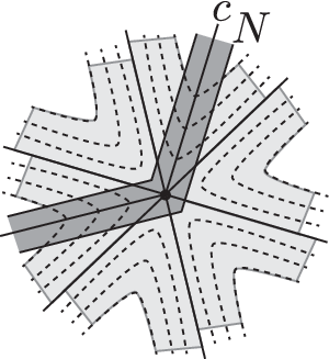
Let $\mu=\mu_{H}$ be the transverse measure to $H$ . We cover $c$ by closed rectangles $\{R_{i}\}_{i=1}^{N}$ in terms of $\omega$ such that (1) ${\rm Int}(R_{i})\cap{\rm Int}(R_{j})=\emptyset$ for $i\neq j$ and the interior of each $R_{i}$ does not contains critical points and points of $P$ ; (2) the vertical segment parts of $c$ is contained in $\partial R_{i}$ for some $i\in I$ , and; (3) $c$ intersects $\partial R_{i}$ only at the interiors of the vertical edges of $R_{i}$ for all $i=1$ , $\cdots$ , $N$ . Let $N$ be a sufficiently narrow annular neighborhood of $c$ such that $N$ is contained in the interior of the union $R=\cup_{i=1}^{N}R_{i}$ and $N$ intersects $\partial R_{i}$ only at the interior of the vertical edges of $R_{i}$ . We may assume that for $i\in I$ , any component of $N\cap R_{i}$ is either one which connects two vertical sides or a half-disk neighborhood of a critical point or a point in $P$ in $\partial R_{i}$ (cf. Figure 2).

Let $U_{0}\cup U_{1}=R\setminus N$ such that $U_{0}$ lies the left of $c$ . Under this convention, an oriented vertical segment in an rectangle $R_{i}$ intersects $c$ goes from $U_{0}$ to $U_{1}$ if $c$ is decreasing. Take a $C^{\infty}$ function $\varphi$ on $R$ such that $0\leq\varphi\leq 1$ , $\varphi=0$ on $U_{0}$ and $\varphi=1$ on $U_{1}$ . Then, $\eta_{C}$ is cohomologous to the closed form on $M$ defined by setting $d\varphi$ on $R$ and $0$ otherwise (cf. [29, §II.3]).

Suppose $R_{i}$ is represented as $[0,a_{i}]\times[0,b_{i}]$ on $\mathbb{R}^{2}\cong\mathbb{C}$ under the flat structure of $\omega$ . Let $\tau_{i}$ be the bottom horizontal edge of $R_{i}$ . Let $\ell_{x}$ be the vertical segment in $R_{i}$ emanating $(x,0)$ . By definition,

	$\displaystyle T_{H}\wedge\eta_{C}$	$\displaystyle=\sum_{i=1}^{N}\int_{0}^{a_{i}}\left(\int_{\ell_{x}}\eta_{C}\right)d\mu_{\tau_{i}}(x)=\sum_{i=1}^{N}\int_{0}^{a_{i}}\left(\int_{\ell_{x}}d\varphi\right)d\mu_{\tau_{i}}(x)$
		$\displaystyle=\sum_{i}\int_{0}^{a_{i}}d\mu_{\tau_{i}}(x)=\mu_{H}(c)=i(c,H),$

where the first term of the second line is given by summing all component of $N\cap R_{i}$ which connects vertical sides of $R_{i}$ . Notice in the above calculation that a component of $N\cap R_{i}$ which is a half-disk neighborhood of a point in $Z(\omega)$ in $\partial R_{i}$ does not contribute in the integration. ∎

Proposition 7.2.

Under the above notation, $T_{v(\omega^{2})}={\rm Re}(\omega)$ .

Proof.

We use the notation around (7.1). By definition,, $\mu_{\tau_{i}}=|dx|$ for each $\tau_{i}$ . For any smooth one form $\gamma=Adx+Bdy$ on $M$ ,

	$\displaystyle T_{v(\omega^{2})}\wedge\gamma$	$\displaystyle=\sum_{i\in I}\int_{0}^{a_{i}}\left(\int_{\ell_{x}}\gamma\right)\|dx\|=\sum_{i\in I}\int_{0}^{a_{i}}\left(\int_{\ell_{x}}Bdy\right)\|dx\|$
		$\displaystyle=\sum_{i\in I}\int_{0}^{a_{i}}\int_{0}^{b_{i}}Bdxdy=\sum_{i\in I}\iint_{R_{i}}{\rm Re}(\omega)\wedge\gamma=\iint_{M}{\rm Re}(\omega)\wedge\gamma,$

which implies what we wanted. ∎

7.3. Double branched covering spaces

Let $x_{0}=(M_{0},f_{0})\in\mathcal{T}_{g,m}$ and $q_{0}\in\mathcal{Q}_{x_{0}}$ . Let $\pi_{q_{0}}\colon\tilde{M}_{q_{0}}\to M_{0}$ be the double covering space associated to $\sqrt{q_{0}}$ , and $i_{q_{0}}\colon\tilde{M}_{q_{0}}\to\tilde{M}_{q_{0}}$ the covering transformation. The lift of $\sqrt{q_{0}}$ defines a holomorphic $1$ -form $\omega_{q_{0}}$ on $\tilde{M}_{q_{0}}$ . For $\mathbb{K}=\mathbb{Z}$ , $\mathbb{R}$ or $\mathbb{C}$ , we denote by $H_{1}(\tilde{M}_{q_{0}};\mathbb{K})^{\pm}$ the eigen space of the action of $i_{q_{0}}$ for the eigen value $\pm 1$ .

Suppose that $q_{0}$ is not a square of an Abelian differential. For $H\in\mathcal{MF}_{L(v(q_{0}))}$ , the transverse measure $\mu$ to the underlying foliation of $v(q_{0})$ for $H$ is lifted to that for the vertical foliation $\tilde{\mu}$ of $\omega_{q_{0}}$ which is equivariant to the action of the involtion $i_{q_{0}}$ . Namely, Let $\tau$ be a transverse arc to the vertical foliation of $\omega_{q_{0}}$ . Then, for any measurable set $E\subset\tau$ , $\tilde{\mu}_{i_{q_{0}}(\tau)}(i_{q_{0}}(E))=\tilde{\mu}_{\tau}(E)$ . Therefore, the current $T_{\tilde{\mu}}$ defined by the lift $\tilde{\mu}$ satisfies

T_{\tilde{\mu}}(i_{q_{0}}^{*}(\gamma))=-T_{\tilde{\mu}}(\gamma)

for any smooth one form $\gamma$ on $\tilde{M}_{q_{0}}$ since the the action of $i_{q_{0}}$ reverses the orientation of the leaves of the vertical foliation of $\omega_{q_{0}}$ . This means that $T_{\tilde{\mu}}$ vanishes on $H_{1}(\tilde{M}_{q_{0}};\mathbb{K})^{+}$ .

8. Holomorphic coordinates associated to extremal lengths

8.1. Double coverings for essentially complete measured foliations

Henceforth, we assume that $F\in\mathcal{MF}$ is essentially complete. In this case, the section

\mathcal{T}_{g,m}\ni x\mapsto q_{F,x}\in\mathcal{Q}_{g,m}

is smooth.

Fix $x_{0}=(M_{0},f_{0})\in\mathcal{T}_{g,m}$ and set $q_{0}=q_{F,x_{0}}$ . For all $x=(M,f)\in\mathcal{T}_{g,m}$ , the differential $q_{F,x}$ is generic and has $4g-4+m$ simple zeros and $m$ simple poles at marked points. The genus of $\tilde{M}_{q_{0}}$ is equal ${\boldsymbol{\xi}}+g$ where ${\boldsymbol{\xi}}=3g-3+m$ . Let $\tilde{Z}(q_{0})\subset\tilde{M}_{q_{0}}$ be the set consisting of zeros of $\omega_{q_{0}}$ and the preimages of marked points of $M$ . Notice from the discussion in [38, Proposition 2.6] that $H_{1}(\tilde{M}_{q_{0}};\mathbb{K})^{-}$ and $H_{1}(\tilde{M}_{q_{0}},\tilde{Z}(q_{0});\mathbb{K})^{-}$ are naturally isomorphic because of the exact sequence

H_{1}(\tilde{Z}(q_{0});\mathbb{K})^{-}\to H_{1}(\tilde{M}_{q_{0}};\mathbb{K})^{-}\to H_{1}(\tilde{M}_{q_{0}},\tilde{Z}(q_{0});\mathbb{K})^{-}\to H_{0}(\tilde{Z}(q_{0});\mathbb{K})^{-},

and $H_{k}(\tilde{Z}(q_{0});\mathbb{K})^{-}=\{0\}$ for $k=0$ , $1$ , since the involution $i_{q_{0}}$ fixes every points of $\tilde{Z}(q_{0})$ .

For any $x\in\mathcal{T}_{g,m}$ , there is a natural bijection between the set of transverse measures to the underlying foliation of $F$ and that to the underlying foliation of the vertical foliation of $q_{F,x}$ . Hence, for any $x=(M,f)\in\mathcal{T}_{g,m}$ and $H\in\mathcal{MF}_{L(F)}$ , we define a current $T_{H,x}$ on the set of smooth one forms on $\tilde{M}_{q_{F,x}}$ associated to the lift $\tilde{\mu}$ of the transverse measure $\mu$ for $H$ .

8.2. Periods of currents revisited

Since the Teichmüller space is contractible, the surface bundle $\cup_{(M,f)\in\mathcal{T}_{g,m}}M$ is trivial (cf. [8]).

For $x=(M,f)\in\mathcal{T}_{g,m}$ , $M\setminus Z(q_{F,x})$ is the Riemann surface of type $(g,4g-4+2m)$ where $Z(q_{F,x})$ is the zeros of $q_{F,x}$ since each $q_{F,x}$ is generic. The zeros of the differentials $q_{F,x}$ ( $x\in\mathcal{T}_{g,m}$ ) define mutually disjoint $(4g-4+2m)$ -smooth sections of the surface bundle $\cup_{(M,f)\in\mathcal{T}_{g,m}}M$ . This means that the zeros and the poles of $q_{F,x}$ is marked (labeled). By taking the double branched covering space along the sections, we obtain the surface bundle $\cup_{x\in\mathcal{T}_{g,m}}\tilde{M}_{q_{F,x}}\to\mathcal{T}_{g,m}$ which is a trivial bundle. Let $\tilde{\Sigma}_{F}\to\Sigma_{g,m}$ be the double branched covering associated to $F$ , which is branched at the singularities of $F$ (see [58, §4]). Then, there is a homeomorphism $\tilde{f}_{x}\colon\tilde{\Sigma}_{F}\to\tilde{M}_{x}$ respecting the trivialization commutes the diagram

(8.1)

\begin{CD}\tilde{\Sigma}_{F}@>{\tilde{f}_{x}}>{}>\tilde{M}_{q_{F,x}}\\ @V{}V{}V@V{}V{}V\\ \Sigma_{g,m}@>{f}>{}>M\end{CD}

after an appropriate choice of the marking $f$ of $x=(M,f)$ so that $f$ maps the (marked) singularities of $F$ to those of $q_{F,x}$ . The homeomorphism $\tilde{f}_{x}$ induces the identification

(8.2)

H_{1}(\tilde{M}_{q_{F,x}};\mathbb{K})^{\pm}\cong H_{1}(\tilde{\Sigma}_{F};\mathbb{K})^{\pm},\quad H^{1}(\tilde{M}_{q_{F,x}};\mathbb{K})^{\pm}\cong H^{1}(\tilde{\Sigma}_{F};\mathbb{K})^{\pm}

for $x\in\mathcal{T}_{g,m}$ and $\mathbb{K}=\mathbb{Z}$ , $\mathbb{R}$ and $\mathbb{C}$ , which are compatible with the duality. Namely, we denote by the pairing

\int_{C}\xi

for $C\in H_{1}(\tilde{M}_{q_{F,x}};\mathbb{K})$ and $\xi\in H^{1}(\tilde{M}_{q_{F,x}};\mathbb{K})$ . After identifying $H_{1}(\tilde{M}_{q_{F,x}};\mathbb{K})^{\pm}\cong H_{1}(\tilde{\Sigma}_{F};\mathbb{K})^{\pm}$ (via the trivialization of the surface bundle),

\int_{C}\xi=\int_{C}\xi^{\prime}

when $\xi\in H^{1}(\tilde{M}_{q_{F,x}};\mathbb{K})$ and $\xi^{\prime}\in H^{1}(\tilde{\Sigma}_{F};\mathbb{K})$ are identified.

Proposition 8.1.

For any $C\in H_{1}(\tilde{\Sigma}_{F};\mathbb{K})^{-}$ and $H\in\mathcal{MF}_{L(F)}$ , the period of $T_{H,x}$ along $C$ is dependent only on $H$ and $C$ .

Proof.

Indeed, this proposition is proved by using the same argument as that by Hubbard and Masur in [38, Proposition 4.3]. We shall sketch the proof.

It suffices to show that the period of $C$ is locally constant because the Teichmüller space is connected.

Let $x=(M,f)\in\mathcal{T}_{g,m}$ . For a simple closed curve $\alpha\in\mathcal{S}$ and $x=(M,f)\in\mathcal{T}_{g,m}$ , we define a decreasing quasi-transverse curve $\tilde{\alpha}=\tilde{\alpha}_{F,x}$ on $\tilde{M}_{q_{F,x}}$ as follows. We represent $\alpha$ as a quasi-transversal curve to the vertical foliation $v(q_{F,x})$ (we may take the geodesic representative of $\alpha$ with respect to the flat metric $|q_{F,x}|$ . See [87, Theorem 17.4]). Then, $\tilde{\alpha}=\tilde{\alpha}_{F,x}$ is defined by taking a lift of $\alpha$ and by orienting transverse segments in the lift so that they are decreasing. By applying the similar argument in [38, Chapter II, S4], we can see that

H_{1}(\tilde{M}_{q_{F,x}};\mathbb{R})^{-}\cong H_{1}(\tilde{M}_{q_{F,x}},\tilde{Z}(q_{F,x});\mathbb{R})^{-}

is generated by $\{\tilde{\alpha}_{F,x}\mid\alpha\in\mathcal{S}\}$ . We modify $\tilde{\alpha}_{F,x}$ at the self intersection points in $\tilde{M}_{q_{F,x}}\setminus\tilde{Z}(q_{F,x})$ as Figure 3, so that $\tilde{\alpha}_{F,x}$ can be thought of as a union of decreasing quasi-transversal simple closed curves since the modification does not change the homology class (see the proof of [38, Proposition 2.2]). From Proposition 7.1, the period of the lift $\tilde{\alpha}=\tilde{\alpha}_{F,x}$ of $\alpha$ is equal to $2i(F,\alpha)$ .

Since the decreasingness of (simple) closed curves is invariant under a (small) deformation, the period is a constant function around $x$ . ∎

8.3. Embedding into $H^{1}(\tilde{M}_{q_{0}};\mathbb{R})^{-}$

In this section, we identify two branched coverings $\tilde{M}_{q_{0}}\to M_{0}$ and $\tilde{\Sigma}_{F}\to\Sigma_{g,m}$ via (8.1). Under the identifications (8.2), we define $\mathcal{H}_{F}\colon\mathcal{T}_{g,m}\to H^{1}(\tilde{M}_{q_{0}};\mathbb{R})^{-}$ by

(8.3)

\mathcal{H}_{F}(x)=[{\rm Im}(\omega_{q_{F,x}})]

where $[{\rm Im}(\omega_{q_{F,x}})]$ is the cohomology class in $H^{1}(\tilde{M}_{q_{0}};\mathbb{R})^{-}$ corresponding to the closed one form ${\rm Im}(\omega_{q_{F,x}})$ . From Proposition 8.1 and (7.3),

T_{H,x_{0}}\wedge\mathcal{H}_{F}(x)=T_{H,x}\wedge{\rm Im}(\omega_{q_{F,x}})

for $H\in\mathcal{MF}_{L(F)}$ and $x\in\mathcal{T}_{g,m}$ .

The following theorem is recognized as a counter part to Bonahon’s theory on the shearing coordinates on Teichmüller space (cf. [15, Theorem 20]. See also [75, Théoème 6.1]).

Theorem 8.1 (Embedding).

The mapping $\mathcal{H}_{F}\colon\mathcal{T}_{g,m}\to H^{1}(\tilde{M}_{q_{0}};\mathbb{R})^{-}\cong H^{1}(\tilde{\Sigma}_{F};\mathbb{R})^{-}$ is a smooth embedding. The image of $\mathcal{H}_{F}$ is the open cone

\mathcal{C}_{F}=\{\xi\in H^{1}(\tilde{M}_{q_{0}};\mathbb{R})^{-}\mid T_{H,x_{0}}\wedge\xi>0\ \mbox{for $H\in\mathcal{MF}_{L(F)}$}\}.

Proof.

The proof of the non-singularity of the differential of $\mathcal{H}_{F}$ is postponed to §8.6 for the sake of readability. From (7.2), the image of $\mathcal{H}_{F}$ is contained in the cone $\mathcal{C}_{F}$ . We only check here the properness of the mapping $\mathcal{H}_{F}$ .

Let $K\subset\mathcal{C}_{F}$ be a compact set. Since intersection number is continuous and $\mathcal{C}_{F}$ is an open cone with vertex $0$ , from (7.2), there are $\epsilon_{0}=\epsilon_{0}(K)>0$ and $\epsilon_{1}=\epsilon_{1}(K)>0$ such that

(8.4)

\epsilon_{0}\leq T_{H,x_{0}}\wedge\mathcal{H}_{F}(x)=2i(h(q_{F,x}),H)\leq\epsilon_{1}

for $x\in\mathcal{T}_{g,m}$ with $\mathcal{H}_{F}(x)\in K$ , and $H\in\mathcal{MF}_{L(F)}\cap\mathcal{SMF}_{x_{0}}$ .

Let $\{x_{n}=(M_{n},f_{n})\}_{n=1}^{\infty}\subset\mathcal{T}_{g,m}$ with $\mathcal{H}_{F}(x_{n})\in K$ for $n\in\mathbb{N}$ . Let $H_{n}=h(q_{F,x_{n}})\in\mathcal{MF}$ be the horizontal foliation of $q_{F,x_{n}}$ . Then, there is $t_{n}>0$ such that $t_{n}H_{n}$ converges to $G\in\mathcal{MF}-\{0\}$ . From (8.4), $t_{n}$ does not diverge. We claim

Claim 1.

The sequence $\{t_{n}\}_{n=1}^{\infty}$ is bounded from below.

We postpone the proof of Claim 1 after finishing the proof of this theorem. From Claim 1, We may assume that $H_{n}$ converges to $G^{\prime}=t_{0}G$ for some $t_{0}>0$ . From (8.4), $i(G^{\prime},F)\neq 0$ and there is $x_{\infty}\in\mathcal{T}_{g,m}$ such that $h(q_{F,x_{\infty}})=G^{\prime}$ . Since $h(q_{F,x_{n}})=H_{n}\to G^{\prime}$ , $q_{F,x_{n}}\to q_{F,x_{\infty}}$ as $n\to\infty$ . Threfore $x_{n}\to x_{\infty}$ . Thus, we conclude that $\mathcal{H}_{F}$ is proper. ∎

Proof of Claim 1.

Suppose to the contrary that $t_{n}\to 0$ . From (8.4),

i(G,F)=\lim_{n\to\infty}t_{n}i(H_{n},F)=0.

Therefore, $F$ and $G$ are topologically equivalent, that is, the underlying foliations of $F$ and $G$ are isotopic (cf. [82]).

Let $\tau$ be a complete train track on $\Sigma_{g,m}$ carrying $F$ . Since $F$ is essentially complete, $F$ is thought of as an interior point of the transverse measures on $\tau$ (cf. [80, Lemma 3.1.2]). We may assume that each component of $\Sigma_{g,m}\setminus\tau$ contains a unique point of $P$ . Let $V(\tau)\subset\mathcal{MF}$ be the measured foliation carried by $\tau$ . From the above discussion, $G$ is thought of as an interior point of $V(\tau)$ . Hence, $H_{n}$ is carried by $\tau$ for sufficiently large $n$ . Let $\mu_{n}\in V(\tau)$ be the transverse measure associated to $H_{n}$ . The pair $(\tau,\mu_{n})$ is regarded as a weighted graph on $\Sigma_{g,m}$ . The branched covering $\tilde{\Sigma}_{F}\to\Sigma_{g,m}$ induces an orientation covering of $\tilde{\tau}\to\tau$ (cf. [80, §3.2]) and the weighted graph $(\tau,\mu_{n})$ defines a cycle $\tilde{\mu}_{n}$ on $\tilde{\Sigma}_{F}$ (via an orientation of $\tilde{\tau}$ ). After choosing an orientation of $\tilde{\tau}$ appropriately, the homology class $[\tilde{\mu}_{n}]$ in $H_{1}(\tilde{M}_{q_{0}};\mathbb{R})$ is thought of as the dual to $\mathcal{H}_{F}(x_{n})$ in the sense that

(8.5)

\int_{C}\mathcal{H}_{F}(x_{n})=[\tilde{\mu}_{n}]\cdot C

for any $C\in H_{1}(\tilde{M}_{q_{0}};\mathbb{R})$ , where the dot in the right-hand side means the algebraic intersection number.

Let $\beta$ be a simple closed curve on $\Sigma_{g,m}$ which hits $\tau$ efficiently (cf. [80, p.19]). Since $\beta$ intersects $\tau$ only at branches of $\tau$ , $\beta$ is presented by the union of paths connecting singular points of $F$ which intersects $\tau$ only at branches between components containing the singular points (in the presentation, $\beta$ may not be simple). Let $\tilde{\beta}\subset\tilde{\Sigma}_{F}\cong\tilde{M}_{q_{0}}$ be the lift of $\beta$ . We orient each branch of $\tilde{\beta}$ appropriately (as $\tilde{\alpha}_{F,x}$ in the proof of Proposition 8.1) , the homology classs $[\tilde{\beta}]$ is in $H_{1}(\tilde{M}_{q_{0}},\tilde{Z}(q_{0});\mathbb{R})^{-}\cong H_{1}(\tilde{M}_{q_{0}};\mathbb{R})^{-}$ and satisfies $[\tilde{\mu}_{n}]\cdot[\tilde{\beta}]=2i(\beta,H_{n})$ . Since $\mathcal{H}_{F}(x_{n})$ is contained in a compact set $K$ , from (8.5), $i(\beta,H_{n})$ is bounded from above. Therefore,

i(G,\beta)=\lim_{n\to\infty}i(t_{n}H_{n},\beta)=0,

which is a contradiction since $G$ is topologically equivalent to $F$ . ∎

8.4. Coordinates to $\mathbb{R}^{6g-6+2m}$

Let $\{a_{i},b_{i}\}_{i=1}^{{\boldsymbol{\xi}}+g}$ be a canonical homology basis of $H_{1}(\tilde{M}_{q_{0}};\mathbb{R})$ in the sense that $a_{j}\cdot a_{k}=b_{j}\cdot b_{k}=0$ and $a_{j}\cdot b_{k}=\delta_{jk}$ for $1\leq j,k\leq{\boldsymbol{\xi}}+g$ . Suppose thet $\{a_{i},b_{i}\}_{i=1}^{{\boldsymbol{\xi}}+g}$ satisfies

(1)

$\{(\pi_{q_{0}})_{*}(a_{j}),(\pi_{q_{0}})_{*}(b_{j})\}_{j=1}^{g}$ is a canonical homology basis on $H_{1}(M_{q_{0}};\mathbb{Z})$ ; and
(2)

$(i_{q_{0}})_{*}(a_{j})-a_{g+j}=(i_{q_{0}})_{*}(b_{j})-b_{g+j}=0$ , $(i_{q_{0}})_{*}(a_{2g+k})+a_{2g+k}=(i_{q_{0}})_{*}(b_{2g+k})+b_{2g+k}=0$ for $1\leq j\leq g$ and $1\leq k\leq{\boldsymbol{\xi}}-g$ .

We define a canonical homology basis $\{A_{k},B_{k}\}_{k=1}^{{\boldsymbol{\xi}}}$ of $H_{1}(\tilde{M}_{q_{0}};\mathbb{R})^{-}$ by

A_{j}=\begin{cases}{\displaystyle\frac{1}{\sqrt{2}}(a_{j}-a_{g+j})}&(1\leq j\leq g),\\ a_{g+j}&(g+1\leq j\leq{\boldsymbol{\xi}}),\end{cases}\quad B_{j}=\begin{cases}{\displaystyle\frac{1}{\sqrt{2}}(b_{j}-b_{g+j})}&(1\leq j\leq g),\\ b_{g+j}&(g+1\leq j\leq{\boldsymbol{\xi}})\end{cases}

for $j=1,\cdots,{\boldsymbol{\xi}}$ (cf. Figure 4).

Consider mappings $\Phi^{A}$ , $\Phi^{B}\colon\mathcal{T}_{g,m}\to\mathbb{R}^{{\boldsymbol{\xi}}}$ and $\Phi\colon\mathcal{T}_{g,m}\to\mathbb{R}^{2{\boldsymbol{\xi}}}$ defined by

	$\displaystyle\Phi^{A}(x)$	$\displaystyle=\left({\rm Im}\int_{A_{1}}\omega_{q_{F,x}},\cdots,{\rm Im}\int_{A_{{\boldsymbol{\xi}}}}\omega_{q_{F,x}}\right),$
	$\displaystyle\Phi^{B}(x)$	$\displaystyle=\left({\rm Im}\int_{B_{1}}\omega_{q_{F,x}},\cdots,{\rm Im}\int_{B_{{\boldsymbol{\xi}}}}\omega_{q_{F,x}}\right),$
	$\displaystyle\Phi(x)$	$\displaystyle=(\Phi^{A}(x),\Phi^{B}(x)).$

The mapping $\Phi$ factors through $H_{1}(\tilde{M}_{q_{0}};\mathbb{R})^{-}$ with the embedding (8.3). We denote by ${\bf y}=({\bf y}^{A},{\bf y}^{B})=(y^{A}_{1},\cdots,y^{A}_{{\boldsymbol{\xi}}},y^{B}_{1},\cdots,y^{B}_{{\boldsymbol{\xi}}})$ the coordinates of $\mathbb{R}^{2{\boldsymbol{\xi}}}=\mathbb{R}^{{\boldsymbol{\xi}}}\times\mathbb{R}^{{\boldsymbol{\xi}}}$ .

Let $H\in\mathcal{MF}_{L(F)}$ . From Proposition 8.1,

	$\displaystyle{\bf a}^{A}_{H}$	$\displaystyle=\left(\int_{A_{1}}T_{H,x_{0}}\cdots,\int_{A_{{\boldsymbol{\xi}}}}T_{H,x_{0}}\right),$
	$\displaystyle{\bf a}^{B}_{H}$	$\displaystyle=\left(\int_{B_{1}}T_{H,x_{0}}\cdots,\int_{B_{{\boldsymbol{\xi}}}}T_{H,x_{0}}\right)$

depend only on $H$ and $\mathcal{MF}_{L(F)}\ni H\mapsto({\bf a}^{A}_{H},{\bf a}^{B}_{H})\in\mathbb{R}^{2{\boldsymbol{\xi}}}$ is continuous (see also [38, Lemma 4.3]). We define a convex cone

\mathbb{H}_{F}=\bigcap_{H\in\mathcal{MF}_{L(F)}}\{{\bf y}=({\bf y}^{A},{\bf y}^{B})\in\mathbb{R}^{2{\boldsymbol{\xi}}}=\mathbb{R}^{{\boldsymbol{\xi}}}\times\mathbb{R}^{{\boldsymbol{\xi}}}\mid{\bf a}^{A}_{H}({\bf y}^{B})^{T}-{\bf a}^{B}_{H}({\bf y}^{A})^{T}>0\},

where the superscript “ $T$ ” means the transpose of matrices (vectors). From Theorem 8.1 and (7.3), we have

Proposition 8.2 (Coordinates).

The mapping

\Phi\colon\mathcal{T}_{g,m}\to\mathbb{R}^{2{\boldsymbol{\xi}}}

is a diffeomorphism onto the image. The image coincides with $\mathbb{H}_{F}$ .

8.5. Differentials of the periods

We first notice the following variational formula obtained in [70]: For $v\in T_{x}\mathcal{T}_{g,m}$ , let $\lambda\mapsto f(\lambda)\in\mathcal{T}_{g,m}$ be the holomorphic disk defined around $\lambda=0$ with $f(0)=x$ and $f_{*}(\partial/\partial\lambda\mid_{\lambda=0})=v$ . Then

(8.6)

\begin{cases}{\displaystyle\left(\frac{\partial}{\partial\lambda}\int_{C}\omega_{q_{F,f(\cdot)}}\right)_{\lambda=0}}&{\displaystyle=\int_{C}\overline{\frac{\pi_{q_{F,x_{0}}}^{*}(\eta_{v})}{\omega_{q_{F,x_{0}}}}}},\\ {\displaystyle\left(\frac{\partial}{\partial\overline{\lambda}}\int_{C}\omega_{q_{F,f(\cdot)}}\right)_{\lambda=0}}&={\displaystyle-\int_{C}\frac{\pi_{q_{F,x_{0}}}^{*}(\eta_{v})}{\omega_{q_{F,x_{0}}}}}\end{cases}

for $C\in H_{1}(\tilde{M}_{q_{F,x_{0}}};\mathbb{R})^{-}$ (cf. [70, Lemma 4.1]). From Propositions 7.2 and 8.1, $\lambda\mapsto\int_{C}{\rm Re}(\omega_{q_{F,f(\cdot)}})$ is a constant function for each $c\in H_{1}(\tilde{M}_{q_{0}})$ , Hence, when $\lambda=s+it$ , we have

(8.7)	$\displaystyle\frac{\partial}{\partial s}\left({\rm Im}\int_{C}\omega_{q_{F,f(\cdot)}}\right)_{\lambda=0}$	$\displaystyle=-\sqrt{-1}\left(\left.\frac{\partial\left(\chi_{q_{F,f(\lambda)}}(c)\right)}{\partial\lambda}\right\|_{\lambda=0}+\left.\frac{\partial\left(\chi_{q_{F,f(\lambda)}}(c)\right)}{\partial\overline{\lambda}}\right\|_{\lambda=0}\right)$
	$\displaystyle=-\sqrt{-1}\left(\overline{\int_{c}\frac{\pi_{q_{F,x_{0}}}^{}\left(\eta_{v}\right)}{\omega_{q_{F,x}}}}-\int_{c}\frac{\pi_{q_{F,x_{0}}}^{}\left(\eta_{v}\right)}{\omega_{q_{F,x}}}\right)$
	$\displaystyle=-2{\rm Im}\int_{c}\frac{\pi_{q_{F,x_{0}}}^{*}\left(\eta_{v}\right)}{\omega_{q_{F,x}}}.$

Let ${\bf y}\in\mathbb{H}_{F}$ and $x=(M,f)\in\mathcal{T}_{g,m}$ with ${\bf y}=\Phi(x)$ . For $j=1,\cdots,{\boldsymbol{\xi}}$ . let $\varphi^{j}_{F,x}$ be the Abelian differential on $\tilde{M}_{q_{F,x}}$ normalized by $\displaystyle\int_{A_{k}}\varphi^{j}_{F,x}=\delta_{jk}$ for $k=1,\cdots,{\boldsymbol{\xi}}$ . Set

\pi_{jk}=\pi_{jk}({\bf y})=\int_{B_{k}}\varphi^{j}_{F,x}\quad(j,k=1,\cdots,{\boldsymbol{\xi}})

and $\Pi=\Pi({\bf y})=(\boldsymbol{\pi}_{1},\cdots,\boldsymbol{\pi}_{{\boldsymbol{\xi}}})=(\pi_{jk}({\bf y}))$ . From the definition,

(8.8)

\omega_{q_{F,x}}=({\bf a}^{A}_{F}+i{\bf y}^{A})\boldsymbol{\varphi}_{F,x}{}^{T},

where ${\bf y}^{A}=\Phi_{A}(x)$ , ${\bf y}^{B}=\Phi_{B}(x)$ and $\boldsymbol{\varphi}_{F,x}=(\varphi^{1}_{F,x},\cdots,\varphi^{{\boldsymbol{\xi}}}_{F,x})$ . Comparing the $B$ -periods of both sides of (8.8), we have the following relation:

(8.9)

{\bf a}^{B}_{F}+i{\bf y}^{B}=({\bf a}^{A}_{F}+i{\bf y}^{A})\Pi.

8.6. The complex structure on $\mathcal{T}_{g,m}$ under the coordinates

For $j=1,\cdots,{\boldsymbol{\xi}}$ , we define a tangent vector $v_{j}=v_{j}(x)\in T_{x}\mathcal{T}_{g,m}$ by

(8.10)

\displaystyle\varphi^{j}_{F,x}

\displaystyle=2\sqrt{-1}\frac{\pi_{q_{F,x_{0}}}^{*}\left(\eta_{v_{j}(x)}\right)}{\omega_{q_{F,x}}}=-2\frac{\pi_{q_{F,x_{0}}}^{*}\left(\eta_{v_{{\boldsymbol{\xi}}+j}(x)}\right)}{\omega_{q_{F,x}}}

where $\eta_{v_{j}(x)}$ is the $q_{F,x}$ -realization for the tangent vector $v_{j}(x)$ (cf. (3.2)). Since (3.3) is an anti-complex isomorphism, $\sqrt{-1}v_{j}=v_{{\boldsymbol{\xi}}+j}$ and $\sqrt{-1}v_{{\boldsymbol{\xi}}+j}=-v_{j}$ for all $j=1,\cdots,{\boldsymbol{\xi}}$ . Set $\{{\bf v}^{A},{\bf v}^{B}\}$ $=\{(v_{k})_{k=1}^{{\boldsymbol{\xi}}},(v_{k})_{k={\boldsymbol{\xi}}+1}^{2{\boldsymbol{\xi}}}\}$ . From (8.7), we have

\Phi_{*}(\{{\bf v}^{A},{\bf v}^{B}\})=(\partial^{A},\partial^{B})\begin{pmatrix}I_{{\boldsymbol{\xi}}}&0\\ {\rm Re}(\Pi)&{\rm Im}(\Pi)\end{pmatrix}

where $\partial^{A}=(\partial/\partial y^{A}_{1},\cdots,\partial/\partial y^{A}_{{\boldsymbol{\xi}}})$ and $\partial^{B}=(\partial/\partial y^{B}_{1},\cdots,\partial/\partial y^{B}_{{\boldsymbol{\xi}}})$ . Since the matrix in the right-hand side is non-singular, the differential $\Phi_{*}$ of $\Phi$ is non-singular. Therefore, so is the differential of $\mathcal{H}_{F}$ .

Set $\{{\bf V}^{A},{\bf V}^{B}\}=\Phi_{*}(\{{\bf v}^{A},{\bf v}^{B}\})$ . We define an almost complex structure $\mathcal{J}$ on $\mathbb{H}_{F}$ by

(8.11)

\displaystyle\mathcal{J}\left(V_{j}\right)=V_{{\boldsymbol{\xi}}+j},

\displaystyle\quad\mathcal{J}\left(V_{{\boldsymbol{\xi}}+j}\right)=-V_{j}\quad(j=1,\cdots,{\boldsymbol{\xi}})

(cf. [46, §2, Chapter IV]). From (8.11), we see that $\mathcal{J}\circ\Phi_{*}=\Phi_{*}\circ(\sqrt{-1}\times)$ , where $\sqrt{-1}\times$ is the standard complex structure on $\mathcal{T}_{g,m}$ defined by multiplying by $\sqrt{-1}$ . Therefore, $\Phi$ is holomorphic. Thus, from Theorem 8.1, we obtain

Proposition 8.3 (Holomorphic chart).

$\Phi\colon(\mathcal{T}_{g,m},\sqrt{-1}\times)\to(\mathbb{H}_{F},\mathcal{J})$ is biholomorphic.

9. Complex analysis

9.1. PSH exhaustions and Boundary measures

Let $\Omega$ be a domain in $\mathbb{C}^{n}$ . A function $u$ on $\Omega$ is said to be plurisubharmonic (PSH) if for each $a\in\Omega$ and $b\in\mathbb{C}^{n}$ , the function $\lambda\mapsto u(a+\lambda b)$ is subharmonic or identically $-\infty$ on every component of the set $\{\lambda\in\mathbb{C}\mid a+\lambda b\in\Omega\}$ . A function $u$ on $\Omega$ is, by definition, pluriharmonic if $u\in C^{2}(\Omega)$ and the restriction to any complex line that meets $\Omega$ is harmonic. The real part of a holomorphic function on $\Omega$ is pluriharmonic (e.g. [45]). A function $u\colon\Omega\to[-\infty,0)$ is said to be an exhaustion on $\Omega$ if $u^{-1}([-\infty,r))$ is relatively compact in $\Omega$ for $r<0$ . A domain $\Omega\subset\mathbb{C}^{n}$ is said to be hyperconvex if there is a continuous PSH exhaustion $u\colon\Omega\to[-\infty,0)$ (cf. [21, Définition 2.1]).

Let $\Omega$ be a bounded hyperconvex domain in $\mathbb{C}^{n}$ . Let $u\colon\Omega\to[-\infty,0)$ be a continuous PSH-exhaustion on $\Omega$ and set $S_{u}(r)=\{z\in\Omega\mid u(z)=r\}$ and $B_{u}(r)=\{z\in\Omega\mid u(z)<r\}$ . For $r<0$ , there is a Borel measure $\mu_{u,r}$ on $\mathbb{C}^{n}$ supported on $S_{u}(r)$ which satisfies the Lelong-Jensen formula:

(9.1)

\int_{S_{u}(r)}Vd\mu_{u,r}=\int_{B_{u}(r)}V(dd^{c}u)^{n}+\int_{B_{u}(r)}(r-u)dd^{c}V\wedge(dd^{c}u)^{n-1}

for any PSH function $V$ on $\Omega$ , where $d=\partial+\overline{\partial}$ , $d^{c}=\sqrt{-1}(\overline{\partial}-\partial)$ and $dd^{c}=2\sqrt{-1}\partial\overline{\partial}$ (cf. [21, Définition 0.1]).

When $\int_{\Omega}(dd^{c}u)^{n}<\infty$ , there is a Borel measure $\mu_{u}$ on $\mathbb{C}^{n}$ which is supported on $\partial\Omega$ such that $\mu_{u,r}$ converges to $\mu_{u}$ weakly on $\mathbb{C}^{n}$ and $\mu_{u}(\partial\Omega)=\int_{\Omega}(dd^{c}u)^{n}$ . The measure $\mu_{u}$ is called the boundary measure associated to $u$ (cf. [21, Théorème et Définition 3.1]). We will use the following results due to Demailly later.

Proposition 9.1 (Théorème 3.4 in [21]).

Let $\Omega$ be a bounded hyperconvex domain in $\mathbb{C}^{N}$ . Let $u,v\colon\Omega\to(-\infty,0]$ be PSH exhaustion. Suppose that $u\leq v$ and $\int_{\Omega}(dd^{c}u)^{N}<\infty$ . Then

\int_{\Omega}(dd^{c}v)^{N}\leq\int_{\Omega}(dd^{c}u)^{N}.

and $\mu_{v}\leq\mu_{u}$ on $\partial\Omega$ .

Proposition 9.2 (Théorème 3.8 in [21]).

Let $\Omega$ be a bounded hyperconvex domain in $\mathbb{C}^{n}$ . Let $u,v\colon\Omega\to[-\infty,0)$ be PSH-continuous exhaustions with

\int_{\Omega}(dd^{x}u)^{n},\ \int_{\Omega}(dd^{c}v)^{n}<\infty.

Suppose that there is an relatively open $N_{0}\subset\partial\Omega$ and a function $\lambda\geq 0$ on $N_{0}$ such that for all $z\in N_{0}$ ,

\limsup_{w\to z}\frac{u(z)}{v(z)}=\lambda(z)<\infty.

Then $d\mu_{u}\leq\lambda^{n}d\mu_{v}$ on $N_{0}$ . If the lim-sup is the limit, $d\mu_{u}=\lambda^{n}d\mu_{v}$ on $N_{0}$ .

9.2. Pluricomplex Green function and Pluriharmonic measures

Demailly observed that for any bounded hyperconvex domain $\Omega$ in $\mathbb{C}^{n}$ and $w\in\Omega$ , there is a unique PSH function $g_{\Omega,w}\colon\Omega\to[-\infty,0)$ such that

(1)

$(dd^{c}g_{\Omega,w})^{n}=(2\pi)^{n}\delta_{w}$ , where $\delta_{w}$ is the Dirac measure with support at $w$ ; and
(2)

$g_{\Omega,w}(z)=\sup_{v}\{v(z)\}$ , where the supremum runs over all non-positive PSH function $v$ on $\Omega$ with $v(z)\leq\log\|z-w\|+O(1)$ around $z=w$

(cf. [21, Théorème 4.3]). The function $g_{\Omega}(w,z)=g_{\Omega,w}(z)$ is called the pluricomplex Green function on $\Omega$ . The pluricomplex Green function $g_{\Omega,w}$ is a continuous exhaustion on $\Omega$ for fixed $w\in\Omega$ . For $w\in\Omega$ , the boundary measure associated with $u_{\Omega,w}=(2\pi)^{-n}g_{\Omega,w}$ is called the pluriharmonic measure of point $w$ (cf. [21, (5.2) Définition]). It is known that the pluriharmonic measure of two distinct points are mutually absolutely continuous (cf. [21, (5.3) Théorème]). The pluriharmonic measure of point $w$ provides the following integral formula:

(9.2)

\int_{\partial\Omega}V(\zeta)d\mu_{u_{\Omega,w}}=V(w)+\int_{\Omega}dd^{c}V\wedge|u_{\Omega,w}|(dd^{c}u_{\Omega,w})^{n-1}

for any PSH function $V$ which is continuous on $\overline{\Omega}$ .

10. The Monge-Ampère measure of extremal lengths

10.1. Extremal length functions on the chart and Frames

We discuss with the chart $\Phi$ on $\mathcal{T}_{g,m}$ in Propositions 8.2 and 8.3 for an essentially complete measured foliation $F$ as complex coordinates. For the simplicity we set

\boldsymbol{\epsilon}_{G}({\bf y})={\rm Ext}_{\Phi^{-1}({\bf y})}(G)

for ${\bf y}\in\mathbb{H}_{F}$ and $G\in\mathcal{MF}$ . From (8.9) and Riemann’s bilinear relation, we have

(10.1)

\displaystyle\boldsymbol{\epsilon}_{F}({\bf y})

\displaystyle=\frac{1}{2}\left({\bf a}^{A}_{F}({\bf y}^{B})^{T}-{\bf a}^{B}_{F}({\bf y}^{A})^{T}\right)=\frac{1}{2}\left({\bf a}^{A}_{F}{\rm Im}(\Pi)({\bf a}^{A}_{F})^{T}+{\bf y}^{A}{\rm Im}(\Pi)({\bf y}^{A})^{T}\right)

for ${\bf y}\in\mathbb{H}_{F}$ .

Under the chart $\Phi$ , we define smooth vector fields ${\bf Z}=(Z_{j})_{1\leq j\leq{\boldsymbol{\xi}}}$ and $\overline{{\bf Z}}=(\overline{Z}_{j})_{1\leq j\leq{\boldsymbol{\xi}}}$ , and $1$ -forms $\boldsymbol{\Omega}=(\Omega^{k})_{1\leq k\leq{\boldsymbol{\xi}}}$ and $\overline{\boldsymbol{\Omega}}=(\overline{\Omega}^{k})_{1\leq k\leq{\boldsymbol{\xi}}}$ by

	$\displaystyle({\bf Z},\overline{{\bf Z}})$	$\displaystyle=\left(\frac{1}{2}({\bf V}^{A}-\sqrt{-1}{\bf V}^{B}),\frac{1}{2}({\bf V}^{A}+\sqrt{-1}{\bf V}^{B})\right)=\frac{1}{2}(\partial^{A},\partial^{B})\begin{bmatrix}I_{{\boldsymbol{\xi}}}&I_{{\boldsymbol{\xi}}}\\ \overline{\Pi}&\Pi\end{bmatrix},$
(10.2)		$\displaystyle(\boldsymbol{\Omega},\overline{\boldsymbol{\Omega}})$	$\displaystyle=-\sqrt{-1}(d{\bf y}^{A},d{\bf y}^{B})\begin{bmatrix}\Pi&-\overline{\Pi}\\ -I_{{\boldsymbol{\xi}}}&I_{{\boldsymbol{\xi}}}\end{bmatrix}\begin{bmatrix}{\rm Im}(\Pi)&0\\ 0&{\rm Im}(\Pi)\end{bmatrix}^{-1}.$

From the observations in §8.5 and §8.6, $Z_{k}$ and $\overline{Z}_{k}$ are $(1,0)$ and $(0,1)$ -vector fields, and $\Omega_{k}$ and $\overline{\Omega}_{k}$ are $(1,0)$ and $(0,1)$ -forms on $\mathbb{H}_{F}$ such that $\Omega_{k}(Z_{l})=\overline{\Omega}_{k}(\overline{Z}_{l})=\delta_{kl}$ and $\Omega_{k}(\overline{Z}_{l})=\overline{\Omega}_{k}(Z_{l})=0$ for $k,l=1,\cdots,{\boldsymbol{\xi}}$ . The systems $\{Z_{k}\}_{k=1}^{{\boldsymbol{\xi}}}$ and $\{\Omega_{k}\}_{k=1}^{{\boldsymbol{\xi}}}$ are a smooth frame on the holomorphic tangent bundle and a smooth coframe of the holomorphic cotangent bundle on $\mathbb{H}_{F}$ (and hence on $\mathcal{T}_{g,m}$ ).

Proposition 10.1 ([74]).

The differentials and the Levi-form of the extremal length function of $F$ satisfies the following:

(10.3)	$\displaystyle\left(\partial\boldsymbol{\epsilon}_{F}\right)_{{\bf y}}$	$\displaystyle=-\frac{\sqrt{-1}}{4}\sum_{k=1}^{{\boldsymbol{\xi}}}({\bf a}_{F}^{A}+\sqrt{-1}{\bf y}^{A}){\rm Im}(\boldsymbol{\pi}_{k})\,\Omega^{k},$
(10.4)	$\displaystyle\left(\overline{\partial}\boldsymbol{\epsilon}_{F}\right)_{{\bf y}}$	$\displaystyle=\frac{\sqrt{-1}}{4}\sum_{k=1}^{{\boldsymbol{\xi}}}({\bf a}_{F}^{A}-\sqrt{-1}{\bf y}^{A}){\rm Im}(\boldsymbol{\pi}_{k})\,\overline{\Omega}^{k},$
(10.5)	$\displaystyle\partial\overline{\partial}\boldsymbol{\epsilon}_{F}$	$\displaystyle=\frac{1}{4}\sum_{k,l=1}^{{\boldsymbol{\xi}}}{\rm Im}(\pi_{kl})\,\Omega^{k}\wedge\overline{\Omega}^{l}$

for ${\bf y}\in\mathbb{H}_{F}$ .

The formulas in in Proposition 10.1 are calculated in [74]. For the completeness, we shall check the formulas. We take the tangent vectors $\{v_{j}\}_{j=1,\cdots,{\boldsymbol{\xi}}}$ as §8.6. Let $\mu_{j}$ be a Beltrami differential on $x=(M,f)\in\mathcal{T}_{g,m}$ satisfying $v_{j}(x)=[\mu_{j}]\in T_{x}\mathcal{T}_{g,m}$ for $j=1,\cdots,{\boldsymbol{\xi}}$ . Then,

	$\displaystyle-\int_{M}\mu_{j}q_{F,x}$	$\displaystyle=-\int_{M}\frac{\overline{\eta_{v_{j}}}}{\|q_{F,x}\|}q_{F,x}=-\frac{\sqrt{-1}}{4}\int_{\tilde{M}_{q_{F,x}}}\omega_{q_{F,x_{0}}}\wedge\overline{\frac{\pi_{q_{F,x}}^{*}(\eta_{v_{j}})}{\omega_{q_{F,x}}}}$
		$\displaystyle=\frac{1}{8}\int_{\tilde{M}_{q_{F,x}}}\omega_{q_{F,x}}\wedge\overline{\varphi^{j}_{F,x}}$
		$\displaystyle=\frac{1}{8}\sum_{k=1}^{\tilde{g}}\left(\int_{A_{k}}\omega_{q_{F,x}}\overline{\int_{B_{k}}\varphi^{j}_{F,x}}-\int_{B_{k}}\omega_{q_{F,x}}\overline{\int_{A_{k}}\varphi^{j}_{F,x}}\right)$
		$\displaystyle=\frac{1}{8}\left(({\bf a}_{F}^{A}+\sqrt{-1}{\bf y}^{A})\cdot\overline{\boldsymbol{\pi}_{j}}-({\bf a}_{F}^{A}+\sqrt{-1}{\bf y}^{A})\cdot\boldsymbol{\pi}_{j}\right)$
		$\displaystyle=-\frac{\sqrt{-1}}{4}({\bf a}_{F}^{A}+\sqrt{-1}{\bf y}^{A})\cdot{\rm Im}(\boldsymbol{\pi}_{j}).$

Since $\Phi_{*}(v_{j})=Z_{j}$ , from Gardiner’s formula ([30]), we have (10.3) and (10.4).

Let $v=\sum_{k=1}^{{\boldsymbol{\xi}}}a_{i}v_{j}$ . From Theorem 5.1 in [70], the Levi form $\mathcal{L}(\boldsymbol{\epsilon}_{F})[v,\overline{v}]$ at $x=(M,f)\in\mathcal{T}_{g,m}$ satisfies

	$\displaystyle\mathcal{L}(\boldsymbol{\epsilon}_{F})[v,\overline{v}]$	$\displaystyle=2\int_{M}\frac{\|\eta_{v}\|^{2}}{\|q_{F,x}\|}=2\sum_{j,k=1}^{{\boldsymbol{\xi}}}a_{j}\overline{a_{k}}\int_{M}\frac{\overline{\eta_{v_{j}}}\eta_{v_{k}}}{\|q_{F,x}\|}$
		$\displaystyle=2\sum_{j,k=1}^{{\boldsymbol{\xi}}}a_{j}\overline{a_{k}}\frac{\sqrt{-1}}{4}\int_{\tilde{M}_{q_{F,x}}}\frac{\pi_{q_{F,x}}^{}(\eta_{v_{k}})}{\omega_{q_{F,x}}}\wedge\overline{\frac{\pi_{q_{F,x}}^{}(\eta_{v_{j}})}{\omega_{q_{F,x}}}}$
		$\displaystyle=\frac{1}{4}\sum_{j,k=1}^{{\boldsymbol{\xi}}}{\rm Im}(\pi_{jk})a_{j}\overline{a_{k}}$

from (8.10) since $\Pi$ is symmetric. This implies (10.5).

10.2. Vector fields tangent to Teichmüller disks

We define a $(1,0)$ -vector field ${\bf X}$ on $\mathbb{H}_{F}$ ( $\cong\mathcal{T}_{g,m}$ ) by

(10.6)	$\displaystyle{\bf X}={\bf X}_{{\bf y}}$	$\displaystyle=-2\sqrt{-1}({\bf a}^{A}_{F}-\sqrt{-1}{\bf y}^{A}){\bf Z}$
	$\displaystyle=-\sqrt{-1}({\bf a}^{A}_{F}-\sqrt{-1}{\bf y}^{A})(I_{{\boldsymbol{\xi}}},\overline{\Pi})\begin{pmatrix}(\partial^{A})^{T}\\ (\partial^{B})^{T}\end{pmatrix}$
	$\displaystyle=-({\bf y}^{A}+\sqrt{-1}{\bf a}^{A}_{F})(\partial^{A})^{T}-({\bf y}^{B}+\sqrt{-1}{\bf a}^{B}_{F})(\partial^{B})^{T}$

(cf. (8.9)). The vcctor field ${\bf X}$ is tangent to the Teichmüller disk defined by the Hubbard-Masur differentials with vertical foliation $F$ .

Proposition 10.2.

The tangent vector field ${\bf X}$ corresponds to the $(1,0)$ -vector associated to the infinitesimal Beltrami differential $\overline{q_{F,x}}/|q_{F,x}|$ at $x\in\mathcal{T}_{g,m}$ .

Proof.

Let $x=(M,f)\in\mathcal{T}_{g,m}$ . Let $v\in T_{x}\mathcal{T}_{g,m}$ be the tangent vector associated to the infinitesimal Beltrami differential $\overline{q_{F,x}}/|q_{F,x}|$ . By the defintion of the $q_{F,x}$ -realization, $\eta_{v}=q_{F,x}$ (cf. (3.2)). Let $\lambda\mapsto f(\lambda)$ be a holomorphic disk defined around $\lambda=0$ which satisfies $f(0)=x$ and $f_{*}(\partial/\partial\lambda\mid_{\lambda=0})=v$ . From (8.6),

	$\displaystyle(\Phi^{A}\circ f)_{*}\left(\left.\frac{\partial}{\partial\lambda}\right\|_{\lambda=0}\right)$	$\displaystyle=\frac{1}{2\sqrt{-1}}\left(\int_{A_{i}}\overline{\frac{\pi_{q_{F,x_{0}}}^{}(q_{F,x})}{\omega_{q_{F,x}}}}-\overline{\left(-\int_{A_{i}}\frac{\pi_{q_{F,x_{0}}}^{}(q_{F,x})}{\omega_{q_{F,x}}}\right)}\right)_{i=1}^{{\boldsymbol{\xi}}}$
		$\displaystyle=-\sqrt{-1}({\bf a}^{A}_{F}-\sqrt{-1}{\bf y}^{A}),$
	$\displaystyle(\Phi^{B}\circ f)_{*}\left(\left.\frac{\partial}{\partial\lambda}\right\|_{\lambda=0}\right)$	$\displaystyle=\frac{1}{2\sqrt{-1}}\left(\int_{B_{i}}\overline{\frac{\pi_{q_{F,x_{0}}}^{}(q_{F,x})}{\omega_{q_{F,x}}}}-\overline{\left(-\int_{B_{i}}\frac{\pi_{q_{F,x_{0}}}^{}(q_{F,x})}{\omega_{q_{F,x}}}\right)}\right)_{i=1}^{{\boldsymbol{\xi}}}$
		$\displaystyle=-\sqrt{-1}({\bf a}^{B}_{F}-\sqrt{-1}{\bf y}^{B}).$

This means $\Phi_{*}({\bf v})={\bf X}_{\Phi(x)}$ from (10.6). ∎

10.3. Monge-Ampère measures associated with extremal lengths

From (10.2) and (10.5),

(10.7)		$\displaystyle(dd^{c}\boldsymbol{\epsilon}_{F})^{{\boldsymbol{\xi}}}$	$\displaystyle={\boldsymbol{\xi}}!\left(\frac{\sqrt{-1}}{2}\right)^{{\boldsymbol{\xi}}}\det({\rm Im}(\Pi))\Omega^{1}\wedge\overline{\Omega}^{1}\wedge\cdots\wedge\Omega^{{\boldsymbol{\xi}}}\wedge\overline{\Omega}^{{\boldsymbol{\xi}}}$
		$\displaystyle={\boldsymbol{\xi}}!\,dy^{A}_{1}\wedge dy^{B}_{1}\wedge\cdots\wedge dy^{A}_{{\boldsymbol{\xi}}}\wedge dy^{B}_{{\boldsymbol{\xi}}}.$

Namely, the Monge-Ampère measure of $\boldsymbol{\epsilon}_{F}$ coincides with the constant multiple of the Euclidean measure under the chart.

Set ${\bf W}=-({\bf X}+\overline{{\bf X}})/4$ and ${\bf W}^{c}=({\bf X}-\overline{{\bf X}})/4\sqrt{-1}=\mathcal{J}({\bf W})$ . Then,

(10.8)

\displaystyle{\bf W}=\frac{1}{2}\left({\bf y}^{A}(\partial^{A})^{T}+{\bf y}^{B}(\partial^{B})^{T}\right)\ \ \mbox{and}\ \ {\bf W}^{c}=\frac{1}{2}\left({\bf a}^{A}_{F}(\partial^{A})^{T}+{\bf a}^{B}_{F}(\partial^{B})^{T}\right).

From Proposition 10.1, we have

(10.9)	$\displaystyle d\boldsymbol{\epsilon}_{F}[{\bf W}]$	$\displaystyle=d^{c}\boldsymbol{\epsilon}_{F}[{\bf W}^{c}]=\frac{1}{2}\boldsymbol{\epsilon}_{F},$
(10.10)	$\displaystyle d\boldsymbol{\epsilon}_{F}[{\bf W}^{c}]$	$\displaystyle=d^{c}\boldsymbol{\epsilon}_{F}[{\bf W}]=0,$
(10.11)	$\displaystyle{\bf W}\lrcorner dd^{c}\boldsymbol{\epsilon}_{F}$	$\displaystyle=d^{c}\boldsymbol{\epsilon}_{F},$
(10.12)	$\displaystyle{\bf W}^{c}\lrcorner dd^{c}\boldsymbol{\epsilon}_{F}$	$\displaystyle=-d\boldsymbol{\epsilon}_{F},$
(10.13)	$\displaystyle{\bf W}\lrcorner(dd^{c}\boldsymbol{\epsilon}_{F})^{{\boldsymbol{\xi}}}$	$\displaystyle={\boldsymbol{\xi}}(dd^{c}\boldsymbol{\epsilon}_{F})^{{\boldsymbol{\xi}}-1}\wedge d^{c}\boldsymbol{\epsilon}_{F}$

on $\mathbb{H}_{F}\cong\mathcal{T}_{g,m}$ , where $\lrcorner$ stands for the contraction (e.g. [13]). Define a function ${\bf u}_{G}$ on $\mathcal{T}_{g,m}$ by

{\bf u}_{G}({\bf y})=-\frac{1}{\boldsymbol{\epsilon}_{G}({\bf y})}=-\frac{1}{{\rm Ext}_{\Phi^{-1}({\bf y})}(G)}

for ${\bf y}\in\mathbb{H}_{F}$ and $G\in\mathcal{MF}$ . From [70, Theorem 5.3], ${\bf u}_{G}$ is a continuous PSH-function on $\mathcal{T}_{g,m}$ for all $G\in\mathcal{MF}$ . Notice from (10.9), (10.10), (10.11) and (10.12) that

	$\displaystyle{\bf W}\lrcorner(dd^{c}{\bf u}_{F})$	$\displaystyle=\frac{{\bf W}\lrcorner(\boldsymbol{\epsilon}_{F}dd^{c}\boldsymbol{\epsilon}_{F}-2d\boldsymbol{\epsilon}_{F}\wedge d^{c}\boldsymbol{\epsilon}_{F})}{\boldsymbol{\epsilon}_{F}^{3}}=0,$
	$\displaystyle{\bf W}^{c}\lrcorner(dd^{c}{\bf u}_{F})$	$\displaystyle=\frac{{\bf W}^{c}\lrcorner(\boldsymbol{\epsilon}_{F}dd^{c}\boldsymbol{\epsilon}_{F}-2d\boldsymbol{\epsilon}_{F}\wedge d^{c}\boldsymbol{\epsilon}_{F})}{\boldsymbol{\epsilon}_{F}^{3}}=0.$

Hence, the $(1,0)$ -vector field ${\bf X}$ on $\mathbb{H}_{F}$ is in the null-space of the complex Hessian $dd^{c}{\bf u}_{F}$ of ${\bf u}_{F}$ , and ${\bf u}_{F}$ satisfies the homogeneous Monge-Ampère equation

(dd^{c}{\bf u}_{F})^{{\boldsymbol{\xi}}}=0

on $\mathbb{H}_{F}\cong\mathcal{T}_{g,m}$ (cf. [45, §3.1]). From (10.13), we obtain

(10.14)

\displaystyle\left(dd^{c}{\bf u}_{F}\right)^{{\boldsymbol{\xi}}-1}\wedge d^{c}{\bf u}_{F}

\displaystyle=\frac{(dd^{c}\boldsymbol{\epsilon}_{F})^{{\boldsymbol{\xi}}-1}\wedge d^{c}\boldsymbol{\epsilon}_{F}}{(\boldsymbol{\epsilon}_{F})^{2{\boldsymbol{\xi}}}}=\frac{1}{{\boldsymbol{\xi}}}{\bf W}\lrcorner\left(\frac{(dd^{c}\boldsymbol{\epsilon}_{F})^{{\boldsymbol{\xi}}}}{(\boldsymbol{\epsilon}_{F})^{2{\boldsymbol{\xi}}}}\right).

In particular $(dd^{c}{\bf u}_{F})^{{\boldsymbol{\xi}}-1}\neq 0$ .

10.4. Measures on the horospheres

For $G\in\mathcal{MF}$ and $R>0$ , we define the horosphere for $G$ by

\displaystyle{\rm HS}(G;R)=\{x\in\mathcal{T}_{g,m}\mid{\rm Ext}_{x}(G)=R^{2}\}.

From (10.1), under the coordinates in Proposition 8.2, the horosphere ${\rm HS}(F;R)$ is represented as the affine subspace

(10.15)

\{({\bf y}^{A},{\bf y}^{B})\in\mathbb{H}_{F}\mid{\bf a}^{A}_{H}({\bf y}^{B})^{T}-{\bf a}^{B}_{H}({\bf y}^{A})^{T}=2R^{2}\}.

Henceforth, we also denote by ${\rm HS}(F;R)$ the set (10.15) under the coordinates in Proposition 8.2. From Proposition 10.2, the tangent vector field ${\bf W}$ is the gradient vector field of the extremal length function for $F$ . From (10.14), the contraction

(10.16)

d{\bf m}_{F,R}=\frac{1}{{\boldsymbol{\xi}}}{\bf W}\lrcorner\left(\frac{(dd^{c}\boldsymbol{\epsilon}_{F})^{{\boldsymbol{\xi}}}}{(\boldsymbol{\epsilon}_{F})^{2{\boldsymbol{\xi}}}}\right)=\left(dd^{c}{\bf u}_{F}\right)^{{\boldsymbol{\xi}}-1}\wedge d^{c}{\bf u}_{F}

is a non-trivial Borel measure on the horosphere ${\rm HS}(F;R)$ . Let $t\in\mathbb{R}$ , we set $T_{t}({\bf y})=e^{2t}{\bf y}$ . From (10.1), (10.8) and (10.16),

(10.17)

{\bf m}_{F,e^{2t}R}(T_{t}(E))={\bf m}_{F,R}(E)

for all Borel set $E\subset{\rm HS}(F,R)$ . From (10.16) and (10.17),

(10.18)

{\bf m}_{F,R}(E)\asymp\int_{\hat{E}}(dd^{c}\boldsymbol{\epsilon}_{F})^{{\boldsymbol{\xi}}}

holds for any Borel set $E\subset{\rm HS}(F,R)$ and $R>0$ , where $\hat{E}=\{T_{t-\log(\sqrt{2}R)}({\bf y})\in\mathbb{H}_{F}\mid{\bf y}\in E,0\leq t\leq(\log 2)/2\}$ and the constants for the comparison depend only on the topology of $\Sigma_{g,m}$ .

10.5. Comparison between ${\bf m}_{F,R}$ and $\hat{\mu}_{Th}^{x_{0}}$

Consider a mapping

(10.19)

\Psi\colon\mathbb{H}_{F}\ni{\bf y}\mapsto h(q_{F,\Phi^{-1}({\bf y})})\in\mathcal{MF}.

Since the piecewise linear structure on $\mathcal{MF}$ is determined by the intersection number function associated with some finite system of simple closed curves, the mapping (10.19) is a piecewise linear homeomorphism onto its image (cf. [16], [23, Exposé 6 and Appendice] and [82]). Hence the pushforward measure $\Psi_{*}(\left(dd^{c}\boldsymbol{\epsilon}_{F}\right)^{{\boldsymbol{\xi}}})$ via the mapping (10.19) is locally comparable with the Thurston measure $\mu_{Th}$ . Compare another treatment of $\mu_{Th}$ due to Masur in [58, §4].

Let $\mathcal{PMF}^{F}\subset\mathcal{PMF}$ be the projection of the image $\Psi(\mathbb{H}_{F})\subset\mathcal{MF}-\{0\}$ . $\mathcal{PMF}^{F}$ consists of the projective classes of measured foliations transverse to $F$ . For $x\in\mathcal{T}_{g,m}$ , let $\mathcal{SMF}_{x}^{F}\subset\mathcal{SMF}_{x}$ be the corresponding subset via the identification $\mathcal{SMF}_{x}\cong\mathcal{PMF}$ discussed in §6.2. The set $\mathcal{SMF}^{F}_{x}$ is an open subset of $\mathcal{SMF}_{x}$ . For $R>0$ , we define a homeomorphism

(10.20)

{\bf T}_{R,x}\colon\mathcal{SMF}_{x}^{F}\to{\rm HS}(F,R)

in such a way that for $G\in\mathcal{SMF}_{x}^{F}$ , $\Psi({\bf T}_{R,x}(G))$ is projectively equivalent to $G$ in $\mathcal{MF}$ .

Proposition 10.3 (Comparison between ${\bf m}_{F,R}$ and $\hat{\mu}_{Th}^{x}$ ).

Let $x\in\mathcal{T}_{g,m}$ . Let $G_{0}\in\mathcal{SMF}_{x}$ such that $G_{0}$ and $F$ are transverse. Let $U$ be a neighborhood of $G_{0}$ with $\overline{U}\subset\mathcal{SMF}^{F}_{x}$ . Then,

{\bf m}_{F,R}({\bf T}_{R,x}(E))\asymp\hat{\mu}_{Th}^{x}(E)

for all $R>0$ and all Borel set $E$ on $U$ , where $\asymp$ means that the measures are comparable with constants independent of the choice of the set $E$ in $U$ , but may depend on $U$ .

Proof.

Since the image ${\bf T}_{R,x}(U)$ is relatively compact in $\mathbb{H}_{F}$ , from the above discussion and (10.18), the measure ${\bf m}_{F,R}$ is comparable with the pushforward measure $({\bf T}_{R,x})_{*}(\hat{\mu}_{Th}^{x})$ on ${\bf T}_{R,x}(U)$ . From (10.17) (or (10.18) again), the constants for the comparison are independent of $R>0$ . ∎

10.6. Monge-Ampère mass of reciprocal of extremal length

Krushkal [50] observed that the pluricomplex Green function $g_{\mathcal{T}_{g,m}}$ on $\mathcal{T}_{g,m}$ is represented as

(10.21)

g_{\mathcal{T}_{g,m}}(x,y)=\log\tanh d_{T}(x,y)\quad(x,y\in\mathcal{T}_{g,m}).

Proposition 10.4.

When $G,H\in\mathcal{MF}$ are transverse, the function ${\bf u}_{G,H}$ is a continuous and negative PSH-exhaustion on $\mathcal{T}_{g,m}$ , and satisfies

(10.22)

u_{G,H}(x)\asymp-e^{-2d_{T}(x_{0},x)}\quad(x\in\mathcal{T}_{g,m}),

where the constants for the comparison depend only on $G$ , $H$ and $x_{0}$ .

Proof.

Since $G$ and $H$ are transverse, there is an $\epsilon_{0}>0$ such that $i(G,J)^{2}+i(H,J)^{2}\geq\epsilon_{0}$ for all $J\in\mathcal{SMF}_{x_{0}}$ . Minsky’s inequality (4.6) implies

{\rm Ext}_{x}(G)+{\rm Ext}_{x}(H)\geq(i(G,J)^{2}+i(H,J)^{2})/{\rm Ext}_{x}(J)\geq\epsilon_{0}/{\rm Ext}_{x}(J).

From Teichmüller’s theorem, for any $x\in\mathcal{T}_{g,m}-\{x_{0}\}$ , there is a unique $J\in\mathcal{SMF}_{x_{0}}$ satisfying ${\rm Ext}_{x}(J)=e^{-2d_{T}(x_{0},x)}$ (cf. [40, §5.2.3]). From (4.3)

(10.23)

\epsilon_{0}e^{2d_{T}(x_{0},x)}\leq{\rm Ext}_{x}(G)+{\rm Ext}_{x}(H)\leq({\rm Ext}_{x_{0}}(G)+{\rm Ext}_{x_{0}}(H))e^{2d_{T}(x_{0},x)}.

Since extremal length functions are positive functions,

(10.24)

-\frac{2}{{\rm Ext}_{x}(G)+{\rm Ext}_{x}(H)}\leq u_{G,H}(x)\leq-\frac{1}{{\rm Ext}_{x}(G)+{\rm Ext}_{x}(H)}

for all $x\in\mathcal{T}_{g,m}$ . The comparison (10.22) follows from (10.23) and (10.24). ∎

Let $K$ be a compact set in $\mathcal{T}_{g,m}$ containing $x_{0}$ in the interior. From the Krushkal formula (10.21) and Proposition 10.4, we have

(10.25)

g_{\mathcal{T}_{g,m}}(x_{0},x)\asymp-e^{-2d_{T}(x_{0},x)}\asymp{\bf u}_{G,H}(x)\quad(x\in\mathcal{T}_{g,m}-K),

where the constants for the first comparison depend only on $K$ .

Proposition 10.5 (Finiteness of MA-mass and Boundary measure for ${\bf u}_{G,H}$ ).

When $G,H\in\mathcal{MF}$ are transverse,

\int_{\mathcal{T}_{g,m}}(dd^{c}{\bf u}_{G,H})^{{\boldsymbol{\xi}}}<\infty,

and the boundary measure $\mu_{{\bf u}_{G,H}}$ of ${\bf u}_{G,H}$ and the pluriharmonic measure are comparable on the Bers boundary in the sense that they are mutually absolutely continuous and the Radon-Nikodym derivatives are bounded.

Proof.

We identify $\mathcal{T}^{B}_{x_{0}}$ with $\mathcal{T}_{g,m}$ via the Bers embedding (cf. §5.2). Fix $r<0$ . We set

g_{\mathcal{T}_{g,m},x_{0};r}(x)=\max\{r,g_{\mathcal{T}_{g,m}}(x_{0},x)\}.

Then, $g_{\mathcal{T}_{g,m},x_{0};r}$ is a continuous PSH-exhaustion on $\mathcal{T}_{g,m}$ . Since $g_{\mathcal{T}_{g,m},x_{0};r}$ coincides with $g_{\mathcal{T}_{g,m}}(x_{0},\,\cdot\,)$ in the outside of a compact set containing $x_{0}$ ,

\int_{\mathcal{T}_{g,m}}(dd^{c}g_{\mathcal{T}_{g,m},x_{0};r})^{{\boldsymbol{\xi}}}<\infty.

Since both $g_{\mathcal{T}_{g,m},x_{0};r}(x)$ and ${\bf u}_{G,H}(x)$ are negative bounded continuous exhaustions, from (10.25), there is a constant $A=A(G,H,x_{0},r)$ , $B=B(G,H,x_{0},r)>0$ such that

Ag_{\mathcal{T}_{g,m},x_{0};r}(x)<{\bf u}_{G,H}(x)<Bg_{\mathcal{T}_{g,m},x_{0};r}(x)\quad(x\in\mathcal{T}_{g,m}).

From Proposition 9.1, the Monge-Ampère mass of ${\bf u}_{G,H}$ is finite. Since $g_{\mathcal{T}_{g,m},x_{0};r}$ coincides with the pluricomplex Green function outside a compact set, the boundary measure of ${\bf u}_{G,H}$ and the pluriharmonic measure are comparable on the Bers boundary. ∎

10.7. Behavior of ${\bf u}_{F,G}$ and ${\bf u}_{F}$ around $\partial\mathcal{T}_{g,m}$

We continue to identify $\mathcal{T}^{B}_{x_{0}}$ with $\mathcal{T}_{g,m}$ via the Bers embedding. Let $\Gamma_{0}$ be the marked Fuchsian group representing $x_{0}$ as §5.2.

Proposition 10.6.

For any $\varphi\in\partial\mathcal{T}^{B}_{x_{0}}$ , there are $F,G\in\mathcal{MF}$ and a neighborhood $\hat{N}$ of $\varphi$ in $A_{2}(\mathbb{H}^{*},\Gamma_{0})$ such that

(1)

$F$ is essentially complete and $F$ and $G$ are transverse;
(2)

for any $x\in\mathcal{T}_{g,m}$ , $(\Xi_{x_{0}}\circ\boldsymbol{\psi}_{x})^{-1}(\hat{N})$ is contained in an open set $\mathcal{SMF}_{x}$ which is relatively compact in $\mathcal{SMF}^{F}_{x}$ ; and
(3)

${\bf u}_{F,G}(x)={\bf u}_{F}(x)$ for $x\in\hat{N}\cap\mathcal{T}^{B}_{x_{0}}$ .

Proof.

Take an essentially complete $F\in\mathcal{MF}$ whose support is realizable in the Kleinian manifold associated to $\varphi$ , that is, ${\rm leng}_{\rho_{\varphi}}(F)>0$ . Since the length function is continuous on the Bers compactification, we can take a small neighborhood $\hat{N}$ of $\varphi$ in $A_{2}(\mathbb{H}^{*},\Gamma_{0})$ such that the ending laminations of the Kleinian surface groups in the closure of $\hat{N}\cap\mathcal{T}^{B}_{x_{0}}$ does not coincide with $L(F)$ (see also [15, Lemma 30]). One can check that such an $\hat{N}$ satisfies the condition (2).

We claim

Claim 2.

For any $G^{\prime}\in\mathcal{MF}$ , the quotient ${\rm Ext}_{x}(G^{\prime})/{\rm Ext}_{x}(F)$ is bounded on $\hat{N}\cap\mathcal{T}^{B}_{x_{0}}$ .

Proof of Claim 2.

Take a sequence $\{x_{n}\}_{n}$ in $\hat{N}\cap\mathcal{T}^{B}_{x_{0}}$ such that

{\rm Ext}_{x_{n}}(G^{\prime})/{\rm Ext}_{x_{n}}(F)\to\sup_{x\in\hat{N}\cap\mathcal{T}^{B}_{x_{0}}}\left({\rm Ext}_{x}(G^{\prime})/{\rm Ext}_{x}(F)\right).

For our purpose, we may assume that $\{x_{n}\}_{n}$ is a divergent sequence in $\mathcal{T}^{B}_{x_{0}}$ . Let $G_{x_{n}}\in\mathcal{SMF}_{x_{0}}$ be the vertical foliation of the quadratic differential (of unit norm) associated to the Teichmüller geodesic connecting from $x_{0}$ to $x_{n}$ . By taking a subsequence, we may assume that $\{x_{n}\}_{n}$ converges to $\varphi_{0}$ in the closure of $\hat{N}\cap\partial\mathcal{T}^{B}_{x_{0}}$ and to $[H_{\infty}]\in\mathcal{PMF}$ in the Thurston compactification, and $\{G_{x_{n}}\}_{n}$ converges to $G_{\infty}\in\mathcal{SMF}_{x_{0}}$ . From [65, Proposition 5.1], $i(G_{\infty},H_{\infty})=0$ .

We claim $i(F,G_{\infty})\neq 0$ . Otherwise, $L(F)=L(G_{\infty})=L(H_{\infty})$ since $F$ is essentially complete (cf. [82]). On the other hand, from [78, Theorem 5.2], the limit $H_{\infty}$ is disjoint from the parabolic loci of the Kleinian manifold asssociated to $\varphi_{0}$ and satisfies $i(H_{\infty},H^{\prime})=0$ for any $H^{\prime}\in\mathcal{MF}$ such that $L(H^{\prime})$ coincides with the ending lamination of a geometrically infinite end of the Kleinian manifold associated to $\varphi_{0}$ . In particular, $L(H_{\infty})$ is not realizable in the Kleinian manifold associated to $\varphi_{0}$ . This contradicts the realizability of $F$ .

Since $i(F,G_{\infty})\neq 0$ , there is a constant $\epsilon_{0}>0$ such that $i(F,G_{x_{n}})\geq\epsilon_{0}$ for sufficiently large $n$ . Hence,

\epsilon_{0}^{2}\leq i(F,G_{x_{n}})^{2}\leq{\rm Ext}_{x_{n}}(F){\rm Ext}_{x_{n}}(G_{x_{n}})=e^{-2d_{T}(x_{0},x_{n})}{\rm Ext}_{x_{n}}(F)

and

\displaystyle\frac{{\rm Ext}_{x_{n}}(G^{\prime})}{{\rm Ext}_{x_{n}}(F)}

\displaystyle\leq\frac{{\rm Ext}_{x_{n}}(G^{\prime})}{\epsilon_{0}^{2}e^{2d_{T}(x_{0},x_{n})}}\leq\frac{{\rm Ext}_{x_{0}}(G^{\prime})}{\epsilon_{0}^{2}}

for sufficiently large $n$ . ∎

Let us complete the proof of Proposition 10.6. Take $G^{\prime}\in\mathcal{MF}$ which is transverse to $F$ . Let $M=\sup_{x}{\rm Ext}_{x}(G^{\prime})/{\rm Ext}_{x}(F)$ for $x\in\hat{N}\cap\mathcal{T}^{B}_{x_{0}}$ and set $G=G^{\prime}/M^{1/2}$ . Then, $F$ and $G$ are transverse and satisfy ${\bf u}_{F,G}(x)={\bf u}_{F}(x)$ for $x\in\hat{N}\cap\mathcal{T}^{B}_{x_{0}}$ . ∎

11. Pluriharmonic measure and Thurston measure

For $x\in\mathcal{T}_{g,m}$ , we denote by ${\boldsymbol{\omega}}^{x_{0}}_{x}$ the pluriharmonic measure of $x$ on $\mathcal{T}^{B}_{x_{0}}$ (cf. §9). The superscript “ $x_{0}$ ” of ${\boldsymbol{\omega}}^{x_{0}}_{x}$ indicates the base point of the Bers slice $\mathcal{T}^{B}_{x_{0}}$ . Since $\partial\mathcal{T}^{B}_{x_{0}}$ is a compact metrizable space, ${\boldsymbol{\omega}}^{x_{0}}_{x}$ and the pushforward measure ${\boldsymbol{\mu}}^{B}_{x}$ defined in (6.5) are inner and outer regular (cf. [12, Theorem 1.1]).

The aim of this section is to prove the following.

Theorem 11.1 (PH measure and Thurston measure).

For any $x\in\mathcal{T}_{g,m}$ , the pluriharmonic measure ${\boldsymbol{\omega}}^{x_{0}}_{x}$ is absolutely continuous with respect to ${\boldsymbol{\mu}}^{B}_{x}$ on $\partial\mathcal{T}^{B}_{x_{0}}$ .

11.1. Cusps are negligible

We first check the following.

Proposition 11.1 (Cusps are negligible).

${\boldsymbol{\omega}}^{x_{0}}_{x}(\partial^{cusp}\mathcal{T}^{B}_{x_{0}})=0$ . Namely, the pluriharmonic measure ${\boldsymbol{\omega}}^{x_{0}}_{x}$ is supported on $\partial^{mf}\mathcal{T}^{B}_{x_{0}}$ .

Proof.

Let $\gamma\in\pi_{1}(\Sigma_{g,m})$ . Let ${\rm APT}^{x_{0}}_{\gamma}\subset\partial\mathcal{T}^{B}_{x_{0}}$ be the boundary groups which admit $\gamma$ as an APT (possibly, ${\rm APT}^{x_{0}}_{\gamma}=\emptyset$ for some $\gamma\in\pi_{1}(\Sigma_{g,m})$ ). Since $\partial^{cusp}\mathcal{T}^{B}_{x_{0}}=\cup_{\gamma\in\pi_{1}(\Sigma_{g,m})}{\rm APT}^{x_{0}}_{\gamma}$ , it suffices to show that ${\boldsymbol{\omega}}^{x_{0}}_{x}({\rm APT}^{x_{0}}_{\gamma})=0$ for each $\gamma\in\pi_{1}(\Sigma_{g,m})$ .

Suppose ${\rm APT}^{x_{0}}_{\gamma}\neq\emptyset$ . Consider a holomorphic function on $\hat{\mathbb{C}}-[0,4]$ defined by

H(w)=\frac{w-2-\sqrt{w^{2}-4w}}{2}

and $H(\infty)=0$ . $H$ maps $\hat{\mathbb{C}}-[0,4]$ conformally onto $\mathbb{D}$ and is continuous on $\hat{\mathbb{C}}-[0,4)$ with $H(4)=1$ . Set

F_{\gamma}(\varphi)=H({\rm tr}^{2}\rho_{\varphi}(\gamma))

for $\varphi\in\overline{\mathcal{T}^{B}_{x_{0}}}$ . Since every monodromy $\rho_{\varphi}$ is faithful and discrete for $\varphi\in\overline{\mathcal{T}^{B}_{x_{0}}}$ , ${\rm tr}^{2}\rho_{\varphi}(\gamma)\in\mathbb{C}-[0,4)$ for all $\varphi\in\overline{\mathcal{T}^{B}_{x_{0}}}$ . Therefore, $F_{\gamma}$ is holomorphic on $\mathcal{T}^{B}_{x_{0}}$ and continuous on the Bers closure $\overline{\mathcal{T}^{B}_{x_{0}}}$ such that $F_{\gamma}(\mathcal{T}^{B}_{x_{0}})\subset\mathbb{D}$ and $F_{\gamma}(\overline{\mathcal{T}^{B}_{x_{0}}})\subset\mathbb{D}\cup\{1\}$ . Furthermore, for $\varphi\in\overline{\mathcal{T}^{B}_{x_{0}}}$ , $\varphi\in{\rm APT}^{x_{0}}_{\gamma}$ if and only if $F_{\gamma}(\varphi)=1$ .

By Demailly’s Poisson integral formula in [21, Théorème 5.1], for all $n\in\mathbb{N}$ , the $n$ -th power $(F_{\gamma})^{n}$ of $F_{\gamma}$ is represented by

(11.1)

(F_{\gamma})^{n}(x)=\int_{\partial\mathcal{T}^{B}_{x_{0}}}(F_{\gamma})^{n}(\varphi){\boldsymbol{\omega}}^{x_{0}}_{x}(\varphi)\quad(x\in\mathcal{T}^{B}_{x_{0}}).

The $n$ -th power $(F_{\gamma})^{n}$ converges pointwise to the characteristic function $\chi_{{\rm APT}^{x_{0}}_{\gamma}}$ of ${\rm APT}^{x_{0}}_{\gamma}$ on $\overline{\mathcal{T}^{B}_{x_{0}}}$ as $n\to\infty$ . Since ${\boldsymbol{\omega}}^{x_{0}}_{x}(\partial\mathcal{T}^{B}_{x_{0}})=1$ and all $(F_{\gamma})^{n}$ is uniformly bounded on the Bers closure, by Lebesgue’s dominated convergence theorem, from (11.1)

0=\int_{\partial\mathcal{T}^{B}_{x_{0}}}\chi_{{\rm APT}^{x_{0}}_{\gamma}}(\varphi)d{\boldsymbol{\omega}}^{x_{0}}_{x}(\varphi)={\boldsymbol{\omega}}^{x_{0}}_{x}({\rm APT}^{x_{0}}_{\gamma}),

and we are done. ∎

11.2. Local comparison and Proof of Theorem 11.1

Let $x\in\mathcal{T}_{g,m}$ . For $H\in\mathcal{SMF}^{mf}_{x}\cong\mathcal{PMF}^{mf}$ , $\varphi_{H}=\varphi_{H,x_{0}}\in\partial\mathcal{T}^{B}_{x_{0}}$ be the totally degenerate group whose ending lamination is equal to $L(H)$ . By Proposition 10.6, there are $F_{H}$ , $G_{H}\in\mathcal{MF}$ and a neighborhood $\hat{N}_{H}$ of $\varphi_{H}$ such that $F_{H}$ is essentially complete, $F_{H}$ and $G_{H}$ are transverse and satisfy

{\bf u}_{F_{H},G_{H}}={\bf u}_{F_{H}}

on $\hat{N}_{H}\cap\mathcal{T}^{B}_{x}$ . Since $\partial\mathcal{T}^{B}_{x_{0}}$ is compact, we can choose a finite system $\{\hat{N}_{H_{i}}\}_{i}$ which covers $\partial\mathcal{T}^{B}_{x_{0}}$ . For the simplicity, set $F_{i}=F_{H_{i}}$ , $G_{i}=G_{H_{i}}$ , and $\hat{N}_{i}=\hat{N}_{H_{i}}$ .

Theorem 11.1 follows from the following proposition.

Proposition 11.2 (Local comparison).

For each $i$ , the pluriharmonic measure ${\boldsymbol{\omega}}^{x_{0}}_{x}$ is absolutely continuous with respect to ${\boldsymbol{\mu}}^{B}_{x}$ on $\partial\mathcal{T}^{B}_{x_{0}}\cap\hat{N}_{i}$ .

Proof.

Since ${\boldsymbol{\omega}}^{x_{0}}_{x}$ and ${\boldsymbol{\mu}}^{B}_{x}$ are outer regular on $\partial\mathcal{T}^{B}_{x_{0}}$ , it suffices to show that

{\boldsymbol{\omega}}^{x_{0}}_{x}(U\cap\hat{N}_{i})\lesssim{\boldsymbol{\mu}}^{B}_{x}(U\cap\hat{N}_{i})

for each relative open set $U\subset\partial\mathcal{T}^{B}_{x_{0}}$ , where the constant for the comparison is independent of $U$ .

For $G\in\mathcal{SMF}_{x}$ which is transverse to $F_{i}$ , let $R_{G}\colon\mathbb{R}\to\mathcal{T}_{g,m}\cong\mathcal{T}^{B}_{x_{0}}$ be the Teichmüller ray defined by $-q_{F_{i},{\bf T}_{1,x}(G)}$ emanating from ${\bf T}_{1,x}(G)\in{\rm HS}(F_{i},1)\subset\mathbb{H}_{F_{i}}\cong\mathcal{T}_{g,m}$ , where ${\bf T}_{1,x}\colon\mathcal{SMF}^{F_{i}}_{x}\to\mathbb{H}_{F_{i}}$ is defined for $F_{i}$ and $R=1$ as (10.20). Let $G^{F_{i}}=h(q_{F_{i},{\bf T}_{1,x}(G)})$ for the simplicity. Then, $G^{F_{i}}$ is projectively equivalent to $G$ , and satisfies ${\rm Ext}_{{\bf T}_{1,x}(G)}(G^{F_{i}})={\rm Ext}_{{\bf T}_{1,x}(G)}(F_{i})=i(G^{F_{i}},F_{i})=1$ .

We define a function $\tau_{i}\colon\partial^{mf}\mathcal{T}^{B}_{x_{0}}\cap\hat{N}_{i}\to\mathbb{R}$ by

\tau_{i}(\varphi_{G})=\inf\{\tau>0\mid\mbox{$R_{G^{\prime}}(t)\in\hat{N}_{i}$ for $t\geq\tau$, $G^{\prime}\in\mathcal{SMF}_{x}^{mf}$ with $L(G^{\prime})=L(G)$}\}.

From Proposition 5.1, $\tau_{i}(\varphi_{G})<\infty$ for any $\varphi_{G}\in\partial^{mf}\mathcal{T}^{B}_{x_{0}}\cap\hat{N}_{i}$ . By the definition of $\tau_{i}$ , $R_{G^{\prime}}(t)\in\hat{N}_{i}$ for all $t>\tau_{i}(\varphi_{G})$ and $G^{\prime}\in\mathcal{SMF}_{x}^{mf}$ with $L(G^{\prime})=L(G)$ .

We claim

Claim 3.

$\tau_{i}$ is upper semicontinuous.

Proof of Claim 3.

Suppose to the contrary that $\tau_{i}$ is not upper semicontinuous at $\varphi_{G}\in\hat{N}_{i}\cap\partial^{mf}\mathcal{T}^{B}_{x_{0}}$ . There are $\epsilon>0$ and $\{H_{n}\}_{n}\subset\mathcal{SMF}_{x}^{mf}$ ( $\cong\mathcal{PMF}^{mf}$ ) such that $\tau(\varphi_{H_{n}})\geq\tau(\varphi_{G})+\epsilon$ and $\varphi_{H_{n}}\to\varphi_{G}$ . Since the Hausdorff limit (in the space of geodesic laminations) of any subsequences of $\{L(H_{n})\}_{n}$ contains $L(G)$ , any accumulation point of $\{H_{n}\}_{n}$ in $\mathcal{SMF}_{x}$ is topologically equivalent to $G$ since $G$ is minimal and filling (see the discussion in the last second paragraph in [35, §1]). Therefore, we may assume that there is a sequence $\{t_{n}\}_{n}$ in $\mathbb{R}$ such that $t_{n}\geq\tau(\varphi_{G})+\epsilon/2$ such that $R_{H_{n}}(t_{n})\not\in\hat{N}_{i}$ and $H_{n}\to G^{\prime}\in\mathcal{SMF}_{x}^{mf}$ with $L(G^{\prime})=L(G)$ .

When $\{t_{n}\}_{n}$ is bounded from above, we may also assume that $t_{n}\to t_{\infty}$ . Since ${\bf T}_{1,x}(H_{n})\to{\bf T}_{1,x}(G)$ , $R_{H_{n}}(t_{n})\to R_{G^{\prime}}(t_{\infty})$ (cf. [25, §1.1, Theorem]). Since $t_{\infty}\geq\tau(\varphi_{G})+\epsilon/2$ , $R_{G^{\prime}}(t_{\infty})\in\hat{N}_{i}$ . This is a contradiction.

Suppose $t_{\infty}\to\infty$ . We may assume that $\{R_{H_{n}}(t_{n})\}_{n}$ converges to $\varphi_{\infty}$ in $\overline{\mathcal{T}^{B}_{x_{0}}}$ . By the same discussion as the proof of Proposition 5.1, we have

{\rm leng}_{\rho_{\varphi_{n}}}(H_{n})\lesssim e^{-t_{n}}{\rm Ext}_{{\bf T}_{1,x}(H_{n})}(H_{n})^{1/2}=e^{-t_{n}}i((H_{n})^{F_{i}},F_{i})=e^{-t_{n}},

where $\varphi_{n}\in\mathcal{T}^{B}_{x_{0}}$ is the corresponding point to $R_{H_{n}}(t_{n})$ . From the continuity of the length function, we have ${\rm leng}_{\rho_{\varphi_{\infty}}}(G^{\prime})=0$ . Therefore we obtain $\varphi_{\infty}=\varphi_{G^{\prime}}=\varphi_{G}$ . This is also a contradiction since $\hat{N}_{i}$ is a neighborhood of $\varphi_{G}$ . ∎

Let $U^{mf}=U\cap\partial^{mf}\mathcal{T}^{B}_{x_{0}}$ . For $s>0$ , we define

U^{mf}_{s}=\{\varphi_{G}\in\hat{N}_{i}\cap\partial^{mf}\mathcal{T}^{B}_{x_{0}}\mid\tau_{i}(\varphi_{G})<s/2\}.

Then, $\{U^{mf}_{s}\}_{s}$ and $U^{mf}$ satisfies

(1)

$U^{mf}_{s}\subset U^{mf}_{s^{\prime}}$ for $s<s^{\prime}$ ;
(2)

$U^{mf}\cap\hat{N}_{i}=\cup_{s>0}U^{mf}_{s}$ ;
(3)

$U^{mf}_{s}$ is open in $\partial^{mf}\mathcal{T}^{B}_{x_{0}}$ in the sense that for any $\varphi_{G}\in U^{mf}_{s}$ , there is an open neighborhood $V$ of $\varphi_{G}$ with $V\cap\partial^{mf}\mathcal{T}^{B}_{x_{0}}\subset U^{mf}_{s}$ ; and
(4)

$\mathcal{U}^{mf}_{s}=(\Xi_{x_{0}}\circ\boldsymbol{\psi}_{x})^{-1}(U^{mf}_{s})$ is open in $\mathcal{SMF}^{mf}_{x}$ in the sense that any $G\in\mathcal{U}^{mf}_{s}$ admits a neighborhood $V^{\prime}$ with $V^{\prime}\cap\mathcal{SMF}^{mf}_{x}\subset\mathcal{U}^{mf}_{s}$ .

The third condition follows from Claim 3, and the fourth condition is deduced from the continuity of the mapping $\Xi_{x_{0}}\circ\boldsymbol{\psi}_{x}$ (cf. §5.3 and 6.2). From (2) of Proposition 10.6, each $\mathcal{U}^{mf}_{s}$ is contained in an open set in $\mathcal{SMF}_{x}$ which is relatively compact in $\mathcal{SMF}^{F_{i}}_{x}$ . Such an open set is defined from $(\Xi_{x_{0}}\circ\boldsymbol{\psi}_{x})^{-1}(\hat{N}_{i})$ , and taken independently of $U$ .

Take $s_{0}>0$ satisfying $U^{mf}_{s}\neq\emptyset$ for $s>s_{0}$ . Fix $s>s_{0}$ , we define subsets $\mathcal{R}$ and $\mathcal{R}_{s}$ in $\mathcal{T}^{B}_{x_{0}}\cong\mathcal{T}_{g,m}$ by

	$\displaystyle\mathcal{R}$	$\displaystyle=\{R_{G^{\prime}}(t)\in\mathcal{T}^{B}_{x_{0}}\mid\mbox{$G^{\prime}\in\mathcal{SMF}^{mf}_{x}\cap\mathcal{SMF}_{x}^{F_{i}}$, $t>0$}\},$
	$\displaystyle\mathcal{R}_{s}$	$\displaystyle=\{R_{G^{\prime}}(t)\in\mathcal{T}^{B}_{x_{0}}\mid G^{\prime}\in\mathcal{U}^{mf}_{s},t>0\}.$

From the above discussion, $\mathcal{R}_{s}$ satisfies an open condition in the sense that any $z\in\mathcal{R}_{s}$ admits a neighborhood $V_{z}$ in $\mathcal{T}^{B}_{x_{0}}$ with $V_{z}\cap\mathcal{R}\subset\mathcal{R}_{s}$ . Next we claim

Claim 4.

For $\varphi_{G}\in U^{mf}_{s}\cap\hat{N}_{i}$ , there is a neighborhood $V_{\varphi_{G}}$ in $A_{2}(\mathbb{H}^{*},\Gamma_{0})$ such that $V_{\varphi_{G}}\cap\partial^{mf}\mathcal{T}^{B}_{x_{0}}\subset U^{mf}_{s}\cap\hat{N}_{i}$ and $V_{\varphi_{G}}\cap\mathcal{R}\subset\mathcal{R}_{s}$ .

Proof of Claim 4.

Since $U^{mf}_{s}$ is open, we can take a neighborhood of $\varphi_{G}$ with the first condition. We need to show the existence of a neighborhood of $\varphi_{G}$ with the second condition.

Otherwise, there is a sequence $\{z_{n}\}_{n}\subset\mathcal{R}\cap\hat{N}_{i}$ with $z_{n}\notin\mathcal{R}_{s}$ and $z_{n}\to\varphi_{G}$ in $\overline{\mathcal{T}^{B}_{x_{0}}}$ . Take $t_{n}>0$ and $H_{n}\in\mathcal{SMF}^{mf}_{x}$ with $R_{H_{n}}(t_{n})=z_{n}$ . By taking a subsequence, we may assume that $H_{n}$ converges to some $G^{\prime}\in\mathcal{SMF}_{x}$ as $n\to\infty$ . Then,

{\rm leng}_{\rho_{\varphi_{n}}}((H_{n})^{F_{i}})\lesssim{\rm Ext}_{z_{n}}((H_{n})^{F_{i}})^{1/2}=e^{-t_{n}},

where $\varphi_{n}\in\mathcal{T}^{B}_{x_{0}}$ is the corresponding point to $z_{n}\in\mathcal{T}_{g,m}$ . Since $z_{n}\to\varphi_{G}$ and $G\in\mathcal{SMF}_{x}^{mf}$ , from the continuity of the length function, $G^{\prime}$ is topologically equivalent to $G$ . Therefore, $\varphi_{H_{n}}\to\varphi_{G^{\prime}}=\varphi_{G}$ . This implies that $\varphi_{H_{n}}\in U^{mf}_{s}\cap\hat{N}_{i}$ and $H_{n}\in\mathcal{U}^{mf}_{s}$ for sufficiently large $n$ . This is a contradiction. ∎

Let us proceed the proof of Proposition 11.2. We define an open set in the ambient space $A_{2}(\mathbb{H}^{*},\Gamma_{0})$ by

\mathcal{V}_{s}=\left(\cup_{z\in\mathcal{R}_{s}}V_{z}\right)\cup\left(\cup_{\varphi_{G}\in U^{mf}_{s}}V_{\varphi_{G}}\right).

From the definition,

	$\displaystyle\mathcal{V}_{s}\cap\partial^{mf}\mathcal{T}^{B}_{x_{0}}$	$\displaystyle=U^{mf}_{s}$
	$\displaystyle\mathcal{V}_{s}\cap\mathcal{R}$	$\displaystyle=\mathcal{R}_{s}.$

Since $\mathcal{SMF}^{mf}_{x}$ is a subset of full-measure on $\mathcal{SMF}_{x}$ , from Proposition 10.3,

(11.2)	$\displaystyle{\bf m}_{F,e^{2u}}(\mathcal{V}_{s}\cap{\rm HS}(F_{i},e^{2u}))$	$\displaystyle={\bf m}_{F,e^{2u}}({\bf T}_{e^{2u},x}(\mathcal{U}^{mf}_{s}))$
	$\displaystyle\asymp\hat{\mu}_{Th}^{x}(\mathcal{U}^{mf}_{s})={\boldsymbol{\mu}}^{B}_{x}(U^{mf}_{s})$
	$\displaystyle\leq{\boldsymbol{\mu}}^{B}_{x}(U\cap\hat{N}_{i})$

for all $u>s$ , where the constant for the comparison is independent of $s>s_{0}$ and $U$ . From the definition of the function $\tau_{i}$ ,

(\mathcal{V}_{s}\cap\mathcal{R})\cap{\rm HS}(F_{i},e^{2u})\subset\hat{N}_{i}

for $u>s/2$ . Since ${\bf u}_{F_{i},G_{i}}={\bf u}_{F_{i}}$ on $\hat{N}_{i}$ (Proposition 10.6) and $\mu_{i,u}=\mu_{{\bf u}_{F_{i},G_{i}},-e^{-2u}}$ is supported on the level set $S_{{\bf u}_{F_{i},G_{i}}}(-e^{-2u})$ of ${\bf u}_{F_{i},G_{i}}$ (cf. §9.1),

(11.3)

\mu_{i,u}(\mathcal{V}_{s})={\bf m}_{F,e^{2u}}(\mathcal{V}_{s}\cap{\rm HS}(F_{i},e^{2u}))

when $u$ is sufficiently large. From [21, Théorème et Définition 3.1] and Proposition 10.5, $\mu_{i,u}$ converges weakly to the boundary measure $\mu_{i}$ of ${\bf u}_{F_{i},G_{i}}$ . Hence, from (11.2) and (11.3) we conclude

\mu_{i}(U^{mf}_{s})=\mu_{i}(\mathcal{V}_{s})\leq\liminf_{u\to\infty}\mu_{i,u}(\mathcal{V}_{s})\lesssim{\boldsymbol{\mu}}^{B}_{x}(U\cap\hat{N}_{i})

since $\mathcal{V}_{s}$ is an open set in the ambient space (cf. [12, (iv) of Theorem 2.1]). Since $\{U^{mf}_{s}\}_{s}$ is an increasing sequence of measurable sets and $\cup_{s>0}U^{mf}_{s}=U^{mf}\cap\hat{N_{i}}$ , from Proposition 11.1, from Proposition 10.5, we deduce

	$\displaystyle{\boldsymbol{\omega}}^{x_{0}}_{x}(U\cap\hat{N}_{i})$	$\displaystyle={\boldsymbol{\omega}}^{x_{0}}_{x}(U^{mf}\cap\hat{N}_{i})$
		$\displaystyle\asymp\mu_{i}(U^{mf}\cap\hat{N}_{i})=\lim_{s\to\infty}\mu_{i}(U^{mf}_{s})\lesssim{\boldsymbol{\mu}}^{B}_{x}(U\cap\hat{N}_{i}),$

where the constants for the comparisons are independent of $U$ . ∎

11.3. Corollary of Theorem 11.1

The pushforward measure ${\boldsymbol{\mu}}^{B}_{x}$ is supported on $\partial^{ue}\mathcal{T}_{g,m}$ (cf. §6.3). The Thurston measure $\hat{\mu}_{Th}^{x}$ on $\mathcal{SMF}^{mf}_{x}$ is defined from the Euclidean measure on the train track coordinates. Hence, we can see that ${\boldsymbol{\mu}}^{B}_{x}$ has no atom on $\partial\mathcal{T}^{B}_{x_{0}}$ since the inverse image $(\Xi_{x_{0}}\circ\boldsymbol{\psi}_{x_{0}})^{-1}(\varphi_{G})$ for $\varphi_{G}\in\partial^{mf}\mathcal{T}^{B}_{x_{0}}$ is a proper (linear) subspace in any train track coordinates around $G$ . Thus, from Theorem 11.1, we deduce

Corollary 11.1.

For any $x\in\mathcal{T}_{g,m}$ , the pluriharmonic measure ${\boldsymbol{\omega}}^{x_{0}}_{x}$ is supported on $\partial^{ue}\mathcal{T}^{B}_{x_{0}}$ and has no atom on $\partial\mathcal{T}^{B}_{x_{0}}$ .

12. Pluriharmonic Poisson kernel

The aim of this section is to determine the Poisson kernel for Teichmüller space.

Theorem 12.1 (Poisson kernel).

The function (1.2) is the Poisson kernel. Namely, for $x,y\in\mathcal{T}_{g,m}$ ,

d{\boldsymbol{\omega}}^{x_{0}}_{y}=\mathbb{P}(x,y,\,\cdot\,)d{\boldsymbol{\omega}}^{x_{0}}_{x}

on $\partial\mathcal{T}^{B}_{x_{0}}$ .

Proof.

Since the function (1.2) is reciprocal in the sense that $\mathbb{P}(x,y,\varphi)=\mathbb{P}(y,x,\varphi)^{-1}$ for $x,y\in\mathcal{T}_{g,m}$ and $\varphi\in\partial\mathcal{T}^{B}_{x_{0}}$ , from Demailly’s theorem (Proposition 9.2) and Corollary 11.1, the assertion of the theorem follows from

(12.1)		$\displaystyle\lim_{\mathcal{T}_{g,m}\ni z\to\varphi}\frac{g_{\mathcal{T}_{g,m}}(y,z)}{g_{\mathcal{T}_{g,m}}(x,z)}$	$\displaystyle=\frac{{\rm Ext}_{x}(F_{\varphi})}{{\rm Ext}_{y}(F_{\varphi})},$
(12.2)		$\displaystyle\limsup_{\mathcal{T}_{g,m}\ni z\to\varphi^{\prime}}\frac{g_{\mathcal{T}_{g,m}}(y,z)}{g_{\mathcal{T}_{g,m}}(x,z)}$	$\displaystyle\leq e^{2d_{T}(x,y)}$

for $x,y\in\mathcal{T}_{g,m}$ , $\varphi\in\partial^{ue}\mathcal{T}^{B}_{x_{0}}$ and $\varphi^{\prime}\in\partial\mathcal{T}^{B}_{x_{0}}$ , where $F_{\varphi}\in\mathcal{MF}$ is defined as §1.2.1. Indeed, (12.1) and (12.2) implies that the left-hand side of (12.2) is measurable and integrable on $\partial\mathcal{T}^{B}_{x_{0}}$ with respect to the harmonic measure ${\boldsymbol{\omega}}^{x_{0}}_{x}$ ( $x\in\mathcal{T}_{g,m}$ ) and coincides with our function $\mathbb{P}(x,y,\cdot)$ a.e. on $\partial\mathcal{T}^{B}_{x_{0}}$ from Corollary 11.1.

(12.2) follows from (10.21) and

\frac{g_{\mathcal{T}_{g,m}}(x,z)}{g_{\mathcal{T}_{g,m}}(y,z)}=e^{-2(d_{T}(x,z)-d_{T}(y,z))}(1+o(1))\leq e^{2d_{T}(x,y)}(1+o(1))

as $z\to\varphi^{\prime}\in\partial\mathcal{T}^{B}_{x_{0}}$ . We show (12.1). We claim

Claim 5.

Let $\{x_{n}\}_{n}\subset\mathcal{T}_{g,m}\cong\mathcal{T}^{B}_{x_{0}}$ be a sequence converging to $\varphi\in\partial^{ue}\mathcal{T}^{B}_{x_{0}}$ . Then, $\{x_{n}\}_{n}$ converges to the projective class $[F_{\varphi}]$ in the Gardinar-Masur compactification.

Proof of Claim 5.

This claim follows by applying the discussion in [69, §3]. We give a proof for confirmation.

Take $\alpha_{n}\in\mathcal{S}$ with ${\rm Ext}_{x_{n}}(\alpha_{n})\leq M$ for some constant $M$ depending only on $(g,m)$ (cf. [10, Theorem 1]). By taking a subsequence, we may assume that $t_{n}\alpha_{n}\to F\in\mathcal{MF}-\{0\}$ with some $t_{n}>0$ . Since $x_{n}$ converges to a totally degenerate group without APT, ${\rm Ext}_{x_{0}}(\alpha_{n})\to\infty$ and hence $t_{n}\to 0$ (cf. [1]). By the Bers inequality and (4.5), the hyperbolic length of the geodesic representation of $t_{n}\alpha_{n}$ in the quasifuchsian manifold associated with $x_{n}$ tends to $0$ . From the continuity of the length function, any sublamination of the support of $F$ is non-realizable in the Kleinian manifold associated with $\varphi$ . Hence, the support of $F$ is contained in $F_{\varphi}$ and $i(F,F_{\varphi})=0$ . Thus we have $[F]=[F_{\varphi}]$ in $\mathcal{PMF}$ since $F_{\varphi}$ is uniquely ergodic.

By taking a subsequence if necessary, we may assume that $x_{n}\to\mathfrak{p}\in\partial_{GM}\mathcal{T}_{g,m}$ . From (4.9), we obtain

	$\displaystyle i_{x_{0}}(\mathfrak{p},[F_{\varphi}])$	$\displaystyle=i_{x_{0}}(\mathfrak{p},[F])=\lim_{n\to\infty}i_{x_{0}}(x_{n},[t_{n}\alpha_{n}])$
		$\displaystyle=\lim_{n\to\infty}e^{-d_{T}(x_{0},x_{n})}\frac{{\rm Ext}_{x_{n}}(t_{n}\alpha_{n})^{1/2}}{{\rm Ext}_{x_{0}}(t_{n}\alpha_{n})^{1/2}}$
		$\displaystyle\leq\lim_{n\to\infty}\frac{M^{1/2}t_{n}e^{-d_{T}(x_{0},x_{n})}}{{{\rm Ext}_{x_{0}}(t_{n}\alpha_{n})^{1/2}}}=0.$

From the characterization of uniquely ergodic measured foliations in the Gardiner-Masur compactification, we conclude that $\mathfrak{p}=[F_{\varphi}]$ (cf. [66, Theorem 3]). ∎

Let us finish the proof. From (4.8), (4.9) and the Krushkal formula (10.21),

	$\displaystyle\frac{g_{\mathcal{T}_{g,m}}(y,z)}{g_{\mathcal{T}_{g,m}}(x,z)}$	$\displaystyle=\exp(2(d_{T}(x,z)-d_{T}(y,z)))(1+o(1))$
		$\displaystyle=\exp(2d_{T}(y,x))\exp(-4\langle x\,\|\,z\rangle_{y})(1+o(1))$
		$\displaystyle\to\exp(2d_{T}(y,x))\left(\exp(-d_{T}(y,x))\frac{{\rm Ext}_{x}(F_{\varphi})^{1/2}}{{\rm Ext}_{y}(F_{\varphi})^{1/2}}\right)^{2}$
		$\displaystyle=\frac{{\rm Ext}_{x}(F_{\varphi})}{{\rm Ext}_{y}(F_{\varphi})}$

as $z\to\varphi\in\partial^{ue}\mathcal{T}^{B}_{x_{0}}$ . This implies (12.1). ∎

Remark 12.1.

The Poisson kernel $\mathbb{P}(x,y,\,\cdot\,)$ is not pluriharmonic in the variable $y$ when ${\boldsymbol{\xi}}\geq 2$ . Indeed, when $F\in\mathcal{MF}$ is uniquely ergodic and essentially complete, for $y=(M_{1},f_{1})\in\mathcal{T}_{g,m}$ and $v\in T_{y}\mathcal{T}_{g,m}$ ,

\displaystyle\mathcal{L}(\mathbb{P}(x,\,\cdot\,,F))[v,\overline{v}]

\displaystyle=-{\boldsymbol{\xi}}\frac{{\rm Ext}_{x}(F)^{{\boldsymbol{\xi}}}}{{\rm Ext}_{y}(F)^{{\boldsymbol{\xi}}+1}}\left(2\int_{M_{1}}\frac{|\eta_{v}|^{2}}{|q_{F,y}|}-\frac{{\boldsymbol{\xi}}+1}{{\rm Ext}_{y}(F)}\left|\langle v,q_{F,y}\rangle\right|^{2}\right),

where $\mathcal{L}$ stands for the Levi form and $\eta_{v}\in\mathcal{Q}_{y}$ is the $q_{F,y}$ -realization of $v$ (cf. (3.2) and [70, Theorem 5.1]). When $v$ is represented by the infiniteismal Beltrami differential $\overline{q_{F,y}}/|q_{F,y}|$ , $\eta_{v}=q_{F,y}$ . Hence, the Levi form of $\mathbb{P}(x,\,\cdot\,,F)$ at $y$ is positive in the direction $v$ . However, when $v$ satisfies $\langle v,q_{F,y}\rangle=0$ , the Levi form at $y$ is negative in this direction $v$ .

On the other hand, the Poisson kernel $\mathbb{P}(x,y,\,\cdot\,)$ is plurisubharmonic in the variable $x$ (cf. [70, Corollary 1.1]).

13. The Green formula

The aim of this section is to complete the proof of the Poisson integral formula (Theorem 1.1). Indeed, Theorem 1.1 is derived from the following theorem.

Theorem 13.1 (Green formula).

Let $V$ be a continuous function on the Bers compactification $\overline{\mathcal{T}^{B}_{x_{0}}}$ which is plurisubharmonic on $\mathcal{T}^{B}_{x_{0}}\cong\mathcal{T}_{g,m}$ . Then

\displaystyle V(x)

\displaystyle=\int_{\partial\mathcal{T}^{B}_{x_{0}}}V(\varphi)\mathbb{P}(x_{0},x,\varphi)d{\boldsymbol{\mu}}^{B}_{x_{0}}(\varphi)-\int_{\Omega}dd^{c}V\wedge|g_{x}|(dd^{c}g_{x})^{{\boldsymbol{\xi}}-1},

where $g_{x}(y)=(2\pi)^{-1}\log\tanh d_{T}(x,y)$ . Furthermore, when ${\boldsymbol{\xi}}\geq 2$ ,

V(x)=\int_{\partial\mathcal{T}^{B}_{x_{0}}}V(\varphi)\mathbb{P}(x_{0},x,\varphi)d{\boldsymbol{\mu}}^{B}_{x_{0}}(\varphi)-\int_{\Omega}dd^{c}V\wedge(dd^{c}g_{x})^{{\boldsymbol{\xi}}-2}\wedge dg_{x}\wedge d^{c}g_{x}.

From the definitions of the function $\mathbb{P}$ and the probability measure ${\boldsymbol{\mu}}^{B}_{x_{0}}$ , the first terms of the above Green formulas are dealt with from Thurston theory and Extremal length geometry. It is also possible to discuss the second terms from the topological aspect in Teichmüller theory. Indeed, the Levi form of the pluricomplex Green function has a topological interpretation in terms of the Thurston symplectic form on $\mathcal{MF}$ via Dumas’ Kähler (symplectic) structure on the space of holomorphic quadratic differentials (cf. [71]. See also [24, Theorem 5.8]).

Theorem 13.1 follows from the following theorem, Theorem 12.1, and the Jensen-Lelong formula (9.2) (cf. [21, Théorème 5.1]).

Theorem 13.2 (PH measure is Thurston measure).

For any $x\in\mathcal{T}_{g,m}$ ,

{\boldsymbol{\omega}}^{x_{0}}_{x}={\boldsymbol{\mu}}^{B}_{x}

on $\partial\mathcal{T}^{B}_{x_{0}}$ .

13.1. Measures and the action of ${\rm Mod}_{g,m}$

Since the action of ${\rm Mod}_{g,m}$ extends continuously to $\mathcal{T}^{B}_{x_{0}}\cup\partial^{mf}\mathcal{T}^{B}_{x_{0}}$ , the pushforward measure $[\omega]_{*}{\boldsymbol{\omega}}^{x_{0}}_{x}$ is well-defined for $[\omega]\in{\rm Mod}_{g,m}$ and $x\in\mathcal{T}_{g,m}$ from Corollary 11.1. We first check the following (see the discussion after [21, Définition 5.2] and [21, (5.8) in Théorème 5.4]).

Lemma 13.1 ( ${\rm Mod}_{g,m}$ and PH measure).

For $[\omega]\in{\rm Mod}_{g,m}$ and $x\in\mathcal{T}_{g,m}$

[\omega]_{*}{\boldsymbol{\omega}}^{x_{0}}_{x}={\boldsymbol{\omega}}^{x_{0}}_{[\omega](x)}

on $\partial\mathcal{T}^{B}_{x_{0}}$ .

Proof.

We need to show that for any bounded continuous function $f$ on $A_{2}(\mathbb{H}^{*},\Gamma_{0})$ , $x\in\mathcal{T}_{g,m}$ and $[\omega]\in{\rm Mod}_{g,m}$ ,

\int_{\partial\mathcal{T}^{B}_{x_{0}}}f\circ[\omega]d{\boldsymbol{\omega}}^{x_{0}}_{x}=\int_{\partial\mathcal{T}^{B}_{x_{0}}}f\,d{\boldsymbol{\omega}}^{x_{0}}_{[\omega](x)}

(cf. [12, Theorem 1.2]). We may assume that $f$ is a strictly PSH function of class $C^{2}$ on a neighborhood of the Bers compactification (see the proof of [21, Théorème and Définition 3.1]). For simplicity, we set $g_{x}(y)=(2\pi)^{-1}g_{\mathcal{T}_{g,m}}(x,y)$ as Theorem 13.1.

Since $g_{[\omega](x)}([\omega](y))=g_{x}(y)$ , from the Lelong-Jensen formula (9.1),

(13.1)

\int_{S_{g_{[\omega](x)}}(r)}fd\mu_{g_{[\omega](x)},r}=\int_{S_{g_{x}}(r)}f\circ[\omega]d\mu_{g_{x},r}

for $r<0$ . We define a function $f^{*}$ on $\overline{\mathcal{T}^{B}_{x_{0}}}$ by

f^{*}(\varphi)=\lim_{\delta\to 0}\sup\{f\circ[\omega](\varphi^{\prime})\mid\|\varphi^{\prime}-\varphi\|_{\infty}<\delta,\varphi^{\prime}\in\mathcal{T}^{B}_{x_{0}}\},

where $\|\cdot\|_{\infty}$ is the hyperbolic supremum norm on $A_{2}(\mathbb{H}^{*},\Gamma_{0})$ . Then $f^{*}$ is bounded and upper semicontinuous on $\overline{\mathcal{T}^{B}_{x_{0}}}$ and satisfies $f^{*}=f\circ[\omega]$ on $\mathcal{T}^{B}_{x_{0}}\cup\partial^{mf}\mathcal{T}^{B}_{x_{0}}$ by virtue of the continuity of $[\omega]$ on $\mathcal{T}^{B}_{x_{0}}\cup\partial^{mf}\mathcal{T}^{B}_{x_{0}}$ . Since $\mu_{g_{x},r}$ converges to ${\boldsymbol{\omega}}^{x_{0}}_{x}$ weakly as $r\to 0$ on $A_{2}(\mathbb{H}^{*},\Gamma_{0})$ , from (13.1) and Proposition 11.1,

	$\displaystyle\int_{\partial\mathcal{T}^{B}_{x_{0}}}f\,d{\boldsymbol{\omega}}^{x_{0}}_{[\omega](x)}$	$\displaystyle=\limsup_{r\to 0}\int_{S_{g_{[\omega](x)}}(r)}fd\mu_{g_{[\omega](x)},r}$
		$\displaystyle=\limsup_{r\to 0}\int_{S_{g_{x}}(r)}f\circ[\omega]d\mu_{g_{x},r}$
		$\displaystyle=\limsup_{r\to 0}\int_{S_{g_{x}}(r)}f^{*}d\mu_{g_{x},r}$
		$\displaystyle\leq\int_{\partial\mathcal{T}^{B}_{x_{0}}}f^{*}d{\boldsymbol{\omega}}^{x_{0}}_{x}=\int_{\partial\mathcal{T}^{B}_{x_{0}}}f\circ[\omega]\,d{\boldsymbol{\omega}}^{x_{0}}_{x}$

(cf. [12, Theorem 2.1, Problem 2.6 in Chapter 1]). Applying the similar argument to a bounded lower semicontinuous function

f_{*}(\varphi)=\lim_{\delta\to 0}\inf\{f\circ[\omega](\varphi^{\prime})\mid\|\varphi^{\prime}-\varphi\|_{\infty}<\delta,\varphi^{\prime}\in\mathcal{T}^{B}_{x_{0}}\}

on $\overline{\mathcal{T}^{B}_{x_{0}}}$ , we obtain the reverse inequality. ∎

Next, we show the following.

Lemma 13.2.

For $x\in\mathcal{T}_{g,m}$ and $[\omega]\in{\rm Mod}_{g,m}$ ,

d{\boldsymbol{\mu}}^{B}_{[\omega](x)}=\mathbb{P}(x,[\omega](x),\,\cdot\,)d{\boldsymbol{\mu}}^{B}_{x}\ \mbox{and}\ \ [\omega]_{*}({\boldsymbol{\mu}}^{B}_{x})={\boldsymbol{\mu}}^{B}_{[\omega](x)}.

Proof.

Since ${\rm Vol}_{Th}([\omega](x))={\rm Vol}_{Th}(x)$ , for any bounded continuous function $f$ on $A_{2}(\mathbb{H}^{*},\Gamma_{0})$ ,

	$\displaystyle\int_{\partial\mathcal{T}^{B}_{x_{0}}}f\,d{\boldsymbol{\mu}}^{B}_{[\omega](x)}$	$\displaystyle=\int_{\mathcal{SMF}^{mf}_{[\omega](x)}}f\circ(\Xi_{x_{0}}\circ\boldsymbol{\psi}_{[\omega](x)})d\hat{\mu}_{Th}^{[\omega](x)}$
		$\displaystyle=\int_{\mathcal{SMF}^{mf}_{x}}f\circ(\Xi_{x_{0}}\circ\boldsymbol{\psi}_{[\omega](x)}\circ\boldsymbol{\psi}_{x,[\omega](x)})d\left((\boldsymbol{\psi}_{x,[\omega](x)}^{-1})_{*}\hat{\mu}_{Th}^{[\omega](x)}\right)$
		$\displaystyle=\int_{\mathcal{SMF}^{mf}_{x}}f\circ(\Xi_{x_{0}}\circ\boldsymbol{\psi}_{x}(G))\frac{1}{{\rm Ext}_{[\omega](x)}(G)^{{\boldsymbol{\xi}}}}d\hat{\mu}_{Th}^{x}(G)$
		$\displaystyle=\int_{\partial\mathcal{T}^{B}_{x_{0}}}f(\varphi)\mathbb{P}(x,[\omega](x),\varphi)\,d{\boldsymbol{\mu}}^{B}_{x}(\varphi)$

from (6.4), where $\boldsymbol{\psi}_{x}$ and $\boldsymbol{\psi}_{x,[\omega](x)}$ are homeomorphisms defined in §6.2. This implies the first equation.

Let us prove the second equation. Any element $[\omega]\in{\rm Mod}_{g,m}$ induces a homeomorphism

[\omega]\colon\mathcal{SMF}_{x}\ni G\to[\omega](G)\in\mathcal{SMF}_{[\omega](x)}.

Since the Thurston measure $\mu_{Th}$ is an invariant measure on $\mathcal{MF}$ with respect to the action of ${\rm Mod}_{g,m}$ , for a measurable set $E\subset\mathcal{SMF}_{[\omega](x)}$ ,

	$\displaystyle[\omega]_{*}\hat{\mu}_{Th}^{x}(E)$	$\displaystyle=\hat{\mu}_{Th}^{x}([\omega]^{-1}(E))$
		$\displaystyle=\mu_{Th}(\{tG\mid G\in[\omega]^{-1}(E),\ 0\leq t\leq 1\})/{\rm Vol}_{Th}(x)$
		$\displaystyle=\mu_{Th}([\omega]^{-1}(\{tG\mid G\in E,\ 0\leq t\leq 1\}))/{\rm Vol}_{Th}(x)$
		$\displaystyle=\mu_{Th}(\{tG\mid G\in E,\ 0\leq t\leq 1\})/{\rm Vol}_{Th}([\omega](x))=\hat{\mu}_{Th}^{[\omega](x)}(E).$

Therefore we obtain

	$\displaystyle\int_{\partial\mathcal{T}^{B}_{x_{0}}}f\circ[\omega]\,d{\boldsymbol{\mu}}^{B}_{x}$	$\displaystyle=\int_{\mathcal{SMF}_{x}}f\circ[\omega]\circ(\Xi_{x_{0}}\circ\boldsymbol{\psi}_{x})d\hat{\mu}_{Th}^{x}$
		$\displaystyle=\int_{\mathcal{SMF}_{x}}f\circ(\Xi_{x_{0}}\circ\boldsymbol{\psi}_{[\omega](x)}\circ[\omega])d\hat{\mu}_{Th}^{x}$
		$\displaystyle=\int_{\mathcal{SMF}_{[\omega](x)}}f\circ(\Xi_{x_{0}}\circ\boldsymbol{\psi}_{[\omega](x)})\left(d([\omega]_{*}\hat{\mu}_{Th}^{x})\right)$
		$\displaystyle=\int_{\mathcal{SMF}_{[\omega](x)}}f\circ(\Xi_{x_{0}}\circ\boldsymbol{\psi}_{[\omega](x)})d\hat{\mu}_{Th}^{[\omega](x)}=\int_{\partial\mathcal{T}^{B}_{x_{0}}}f\,d{\boldsymbol{\mu}}^{B}_{[\omega](x)},$

which implies what we wanted. ∎

13.2. Proof of Theorem 13.2

Let $x\in\mathcal{T}_{g,m}$ . From Theorem 11.1, there is an integrable function $\Lambda_{x}$ on $\partial\mathcal{T}^{B}_{x_{0}}$ such that

d{\boldsymbol{\omega}}^{x_{0}}_{x}=\Lambda_{x}d{\boldsymbol{\mu}}^{B}_{x}

on $\partial\mathcal{T}^{B}_{x_{0}}$ . For $[\omega]\in{\rm Mod}_{g,m}$ , from Theorem 12.1, Lemmas 13.1 and 13.2,

	$\displaystyle\mathbb{P}(x,[\omega](x),\,\cdot\,)\Lambda_{x}d{\boldsymbol{\mu}}^{B}_{x}.$	$\displaystyle=\mathbb{P}(x,[\omega](x),\,\cdot\,)d{\boldsymbol{\omega}}^{x_{0}}_{x}=d{\boldsymbol{\omega}}^{x_{0}}_{[\omega](x)}=[\omega]_{*}d{\boldsymbol{\omega}}^{x_{0}}_{x}$
		$\displaystyle=[\omega]_{*}(\Lambda_{x}d{\boldsymbol{\mu}}^{B}_{x})=\Lambda_{x}\circ[\omega]^{-1}d{\boldsymbol{\mu}}^{B}_{[\omega](x)}$
		$\displaystyle=(\Lambda_{x}\circ[\omega]^{-1})\mathbb{P}(x,[\omega](x),\,\cdot\,)d{\boldsymbol{\mu}}^{B}_{x}.$

Therefore, we obtain $\Lambda_{x}\circ[\omega]^{-1}=\Lambda_{x}$ a.e. on $\partial\mathcal{T}^{B}_{x_{0}}$ with respect to ${\boldsymbol{\mu}}^{B}_{x}$ . Hence, the pullback $\Lambda_{x}\circ\Xi_{x}$ is an invariant integrable function on $\mathcal{PMF}$ under the action of ${\rm Mod}_{g,m}$ . Since the action of ${\rm Mod}_{g,m}$ on $\mathcal{PMF}$ is ergodic with respect to the measure class of $(\boldsymbol{\psi}_{x_{0}})_{*}(\hat{\mu}_{Th}^{x_{0}})$ (cf. [58, Corollary 2]), $\Lambda_{x}\circ\Xi_{x}$ is a constant function, and so is $\Lambda_{x}$ as a measurable function on $\partial\mathcal{T}^{B}_{x_{0}}$ . Since both measures ${\boldsymbol{\omega}}^{x_{0}}_{x}$ and ${\boldsymbol{\mu}}^{B}_{x}$ are probability measures on $\partial\mathcal{T}^{B}_{x_{0}}$ , $\Lambda_{x}\equiv 1$ a.e. on $\partial\mathcal{T}^{B}_{x_{0}}$ . ∎

14. Boundary behavior of Poisson integral

The purpose of this section to prove Theorem 1.2.

14.1. Two lemmas

As §11.2, for $H\in\mathcal{SMF}^{mf}_{x_{0}}$ , we denote by $\varphi_{H}\in\partial\mathcal{T}^{B}_{x_{0}}$ the totally degenerate group whose ending lamination is equal to $L(H)$ .

Lemma 14.1.

Let $\varphi_{H}\in\partial^{mf}\mathcal{T}^{B}_{x_{0}}$ . For $\delta>0$ , we define

N(\varphi_{H};\delta)=\{\varphi_{G}\in\partial^{mf}\mathcal{T}^{B}_{x_{0}}\mid i(H,G)<\delta\}.

Then, $N(\varphi_{H};\delta)$ is an open neighborhood of $\varphi_{H}$ in $\partial^{mf}\mathcal{T}^{B}_{x_{0}}$ and satisfies

\bigcap_{\delta>0}N(\varphi_{H};\delta)=\{\varphi_{H}\}.

Proof.

The mapping $\Xi_{x_{0}}\colon\mathcal{PMF}^{mf}\to\partial^{mf}\mathcal{T}^{B}_{x_{0}}$ is factorized as the composition of the homeomorphism from the Gromov-boundary of the complex of curves to $\partial^{mf}\mathcal{T}^{B}_{x_{0}}$ and the measure-forgetting mapping from $\mathcal{PMF}^{mf}$ to the Gromov boundary of the complex of curves (cf. [52, Theorem 6.6]). The measure-forgetting mapping is the quotient mapping (cf. [35] and [44]). Since the intersection number function is continuous, $(\Xi_{x_{0}}\circ\boldsymbol{\psi}_{x_{0}})^{-1}(N(\varphi_{H};\delta))=\{G\in\mathcal{SMF}^{mf}_{x_{0}}\mid i(H,G)<\delta\}$ is open in $\mathcal{SMF}^{mf}_{x_{0}}$ . Hence, $N(\varphi_{H};\delta)$ is an open neighborhood of $\varphi_{H}$ in $\partial^{mf}\mathcal{T}^{B}_{x_{0}}$ .

Let $\varphi_{G}\in\bigcap_{\delta>0}N(\varphi_{H};\delta)\subset\partial^{mf}\mathcal{T}^{B}_{x_{0}}$ . Since $i(G,H)<\delta$ for all $\delta>0$ , $i(G,H)=0$ , and hence $L(G)=L(H)$ since $H$ is minimal and filling. Therefore $\varphi_{G}=\varphi_{H}$ . ∎

Lemma 14.2.

Let $\delta>0$ and $\varphi_{H}\in\partial^{ue}\mathcal{T}^{B}_{x_{0}}$ , there is a neigborhood $U$ of $\varphi_{H}$ in $A_{2}(\mathbb{H}^{*},\Gamma_{0})$ such that

\sup\{\mathbb{P}(x_{0},x,\varphi)\mid\varphi\in\partial^{ue}\mathcal{T}^{B}_{x_{0}}-N(\varphi_{H};\delta)\}\leq\left(\frac{2}{\delta^{2}}\right)^{{\boldsymbol{\xi}}}e^{-2{\boldsymbol{\xi}}d_{T}(x_{0},x)}

for $x\in\mathcal{T}^{B}_{x_{0}}\cap U$ .

Proof.

We first claim that

U^{\prime}=\{x\in\mathcal{T}_{g,m}\mid\mbox{$e^{-2d_{T}(x_{0},x)}{\rm Ext}_{x}(G)\geq\delta^{2}/2$ for $G\in\mathcal{SMF}^{ue}_{x_{0}}$ with $i(H,G)\geq\delta$}\}

satisfies that $U\cap\mathcal{T}^{B}_{x_{0}}\subset U^{\prime}$ for some neighborhood $U$ of $\varphi_{H}$ in is a neighborhood of $\varphi_{H}$ in the sense that there is a neighborhood $U$ of $A_{2}(\mathbb{H}^{*},\Gamma_{0})$ .

Otherwise, there is a sequence $\{x_{n}\}_{n=1}^{\infty}$ in $\mathcal{T}_{g,m}$ converging to $\varphi_{H}$ and $\{G_{n}\}_{n}\subset\mathcal{SMF}^{ue}_{x_{0}}$ such that $e^{-2d_{T}(x_{0},x_{n})}{\rm Ext}_{x_{n}}(G_{n})<\delta^{2}/2$ for some $G_{n}\in\mathcal{SMF}^{ue}_{x_{0}}$ with $i(G_{n},H)\geq\delta$ . We may assume that $G_{n}$ converges to some $G_{0}\in\mathcal{SMF}_{x_{0}}$ . Since the intersection number is continuous, $i(G_{0},H)\geq\delta$ . From Claim 5 in Theorem 12.1, (4.9) and (4.10),

	$\displaystyle\delta^{2}/2$	$\displaystyle>e^{-2d_{T}(x_{0},x_{n})}{\rm Ext}_{x_{n}}(G_{n})=i_{x_{0}}(x_{n},[G_{n}])$
		$\displaystyle\to i_{x_{0}}([H],[G_{0}])=\frac{i(G_{0},H)^{2}}{{\rm Ext}_{x_{0}}(G_{0}){\rm Ext}_{x_{0}}(H)}=i(G_{0},H)^{2}\geq\delta^{2}$

as $n\to\infty$ , which is a contradiction.

We show that the open neighborhood $U$ which is taken above satisfies the desired condition. Indeed, for $x\in U^{\prime}$ , we deduce

\mathbb{P}(x_{0},x,\varphi_{G})=\left(\frac{{\rm Ext}_{x_{0}}(G)}{{\rm Ext}_{x}(G)}\right)^{{\boldsymbol{\xi}}}\leq\left(\frac{2}{\delta^{2}}\right)^{{\boldsymbol{\xi}}}e^{-2{\boldsymbol{\xi}}d_{T}(x_{0},x)}.

Since the right-hand side is independent of $\varphi_{G}\in\partial^{ue}\mathcal{T}^{B}_{x_{0}}-N(\varphi_{H};\delta)$ , we have the assertion. ∎

14.2. Proof of Theorem 1.2

We prove Theorem 1.2 with a weaker assumption. Suppose $V$ is integrable on $\partial\mathcal{T}^{B}_{x_{0}}$ and the restriction of $V$ to $\partial^{mf}\mathcal{T}^{B}_{x_{0}}$ is continuous at $\varphi_{0}\in\partial^{ue}\mathcal{T}^{B}_{x_{0}}$ .

Fix $\epsilon>0$ . From Lemma 14.1, there is $\delta>0$ such that $|V(\varphi)-V(\varphi_{0})|<\epsilon$ for $\varphi\in N(\varphi_{H};\delta)$ . Since $d{\boldsymbol{\mu}}^{B}_{x}=\mathbb{P}(x_{0},x,\cdot)d{\boldsymbol{\mu}}^{B}_{x_{0}}$ is a probability measure on $\partial\mathcal{T}^{B}_{x_{0}}$ for $x\in\mathcal{T}^{B}_{x_{0}}$ ,

(14.1)

\int_{N(\varphi_{H};\delta)}|V(\varphi)-V(\varphi_{0})|\mathbb{P}(x_{0},x,\varphi)d{\boldsymbol{\mu}}^{B}_{x_{0}}(\varphi)<\epsilon.

Since $V$ is integrable on $\partial\mathcal{T}^{B}_{x_{0}}$ and $\partial^{ue}\mathcal{T}^{B}_{x_{0}}$ is of full measure in $\partial\mathcal{T}^{B}_{x_{0}}$ with respect to ${\boldsymbol{\mu}}^{B}_{x_{0}}$ (Corollary 11.1), from Lemma 14.2, there is a neighborhood $U$ of $\varphi_{H}$ in $A_{2}(\mathbb{H}^{*},\Gamma_{0})$ such that

(14.2)

\int_{\partial\mathcal{T}^{B}_{x_{0}}-N(\varphi_{H};\delta)}|V(\varphi)-V(\varphi_{0})|\mathbb{P}(x_{0},x,\varphi)d{\boldsymbol{\mu}}^{B}_{x_{0}}(\varphi)\leq Me^{-2{\boldsymbol{\xi}}d_{T}(x_{0},x)}

for $x\in\mathcal{T}^{B}_{x_{0}}\cap U$ , where $M>0$ depends only on $V$ , $\varphi_{0}$ and $\delta$ . From (14.1) and (14.2), we conclude

		$\displaystyle\left\|\int_{\partial\mathcal{T}^{B}_{x_{0}}}V(\varphi)\mathbb{P}(x_{0},x,\varphi)d{\boldsymbol{\mu}}^{B}_{x_{0}}(\varphi)-V(\varphi_{0})\right\|$
		$\displaystyle\leq\int_{\partial\mathcal{T}^{B}_{x_{0}}}\|V(\varphi)-V(\varphi_{0})\|\mathbb{P}(x_{0},x,\varphi)d{\boldsymbol{\mu}}^{B}_{x_{0}}(\varphi)\leq\epsilon+Me^{-2{\boldsymbol{\xi}}d_{T}(x_{0},x)}$

for $x\in\mathcal{T}^{B}_{x_{0}}\cap U$ . ∎

15. Averaging on $\mathcal{PMF}$

We discuss on the integral representation from the topological point of view.

15.1. Integral representation with $\mathcal{PMF}$

We identify $\mathcal{SMF}_{x_{0}}$ with $\mathcal{PMF}$ as §6.2. We think of $\hat{\mu}_{Th}^{x_{0}}$ as a Borel measure on $\mathcal{PMF}$ under the identification. We define a linear operator (isometry)

L^{1}(\partial\mathcal{T}^{B}_{x_{0}},{\boldsymbol{\mu}}^{B}_{x_{0}})\ni V\mapsto\hat{V}=V\circ\Xi_{x_{0}}\in L^{1}(\mathcal{PMF},\hat{\mu}_{Th}^{x_{0}}).

The following is an immediate consequence from Theorem 1.1.

Corollary 15.1 (Integral representation with $\mathcal{PMF}$ ).

Let $V$ be a pluriharmonic function on $\mathcal{T}_{g,m}$ which is continuous on the Bers closure. Then,

(15.1)

V(x)=\int_{\mathcal{PMF}}\hat{V}([F])\left(\sqrt{\frac{{\rm Ext}_{x_{0}}(F)}{{\rm Ext}_{x}(F)}}\right)^{2{\boldsymbol{\xi}}}d\hat{\mu}_{Th}^{x_{0}}([F])

for $x\in\mathcal{T}_{g,m}$ .

Remark 15.1.

The family of measures

\left\{\left(\sqrt{\frac{{\rm Ext}_{x_{0}}(\cdot)}{{\rm Ext}_{x}(\cdot)}}\right)^{2{\boldsymbol{\xi}}}d\hat{\mu}_{Th}^{x_{0}}\right\}_{x\in\mathcal{T}_{g,m}}

on $\mathcal{PMF}$ which are appeared in the right-hand side (15.1) is already discussed in [4, §2.3.1], and recognized as the conformal density of dimension $2{\boldsymbol{\xi}}=6g-6+2m$ (the Patterson-Sullivan measures) on $\mathcal{T}_{g,m}$ from the dynamical point of view (see also [36]).

We prove Mirzakhani and Dumas’ observation in [24] by using the formulation as in Corollary 15.1 as follows.

Corollary 15.2 (Mirzakhani and Dumas [24]).

The Hubbard-Masur function (6.2) is constant.

Proof.

Fix $x_{0}\in\mathcal{T}_{g,m}$ . Let $x\in\mathcal{T}_{g,m}$ . By applying $V\equiv 1$ on $A_{2}(\mathbb{H}^{*},\Gamma_{0})$ to Corollary 15.1, we obtain

(15.2)		$\displaystyle 1$	$\displaystyle=\int_{\mathcal{PMF}}\left(\frac{{\rm Ext}_{x_{0}}(F)}{{\rm Ext}_{x}(F)}\right)^{{\boldsymbol{\xi}}}d\hat{\mu}_{Th}^{x_{0}}([F])=\int_{\mathcal{SMF}_{x_{0}}}\left(\frac{{\rm Ext}_{x_{0}}(F)}{{\rm Ext}_{x}(F)}\right)^{{\boldsymbol{\xi}}}d\hat{\mu}_{Th}^{x_{0}}(F)$
		$\displaystyle=\frac{1}{{\rm Vol}_{Th}(x_{0})}\int_{\mathcal{BMF}_{x_{0}}}\left(\frac{{\rm Ext}_{x_{0}}(F)}{{\rm Ext}_{x}(F)}\right)^{{\boldsymbol{\xi}}}d\mu_{Th}(F)$

for $x\in\mathcal{T}_{g,m}$ . On the other hand, the mapping

\mathcal{BMF}_{x_{0}}\ni F\mapsto\sqrt{\frac{{\rm Ext}_{x_{0}}(F)}{{\rm Ext}_{x}(F)}}F\in\mathcal{BMF}_{x}

is homeomorphic (the origin is sent to the origin). Therefore, the last term of (15.2) coincides with ${\rm Vol}_{Th}(x)/{\rm Vol}_{Th}(x_{0})$ . ∎

From (6.4) and Corollary 15.2, we also obtain the following.

Corollary 15.3.

For $x,y\in\mathcal{T}_{g,m}$ , after identifying $\mathcal{SMF}_{x}$ and $\mathcal{SMF}_{y}$ with $\mathcal{PMF}$ as §6.2, we have

\hat{\mu}_{Th}^{y}(E)=\int_{E}\left(\frac{{\rm Ext}_{x}(F)}{{\rm Ext}_{y}(F)}\right)^{{\boldsymbol{\xi}}}d\hat{\mu}_{Th}^{x}([F])

for any measurable set $E\subset\mathcal{PMF}$ .

15.2. Phenomena by averaging

In this section, we discuss the averaging procedure from the Poisson integral formula (1.3).

15.2.1. Presentation of differentials by averaging

Let $V$ be a pluriharmonic function on $\mathcal{T}^{B}_{x_{0}}$ which is continuous on the Bers closure. We identify the holomorphic cotangent bundle over $\mathcal{T}_{g,m}$ with the space of holomorphic quadratic differentials as §3.3. The following formula is deduced by the differentiating the both sides of (15.1):

(15.3)	$\displaystyle(\partial V)_{x}$	$\displaystyle={\boldsymbol{\xi}}\int_{\mathcal{PMF}}\hat{V}([F])\left(\frac{{\rm Ext}_{x_{0}}(F)}{{\rm Ext}_{x}(F)}\right)^{{\boldsymbol{\xi}}}\frac{q_{F,x}}{\\|q_{F,x}\\|}\,d\hat{\mu}_{Th}^{x_{0}}([F])$
	$\displaystyle={\boldsymbol{\xi}}\int_{\mathcal{PMF}}\hat{V}([F])\frac{q_{F,x}}{\\|q_{F,x}\\|}\,d\hat{\mu}_{Th}^{x}([F])$
(15.4)	$\displaystyle(\overline{\partial}V)_{x}$	$\displaystyle={\boldsymbol{\xi}}\int_{\mathcal{PMF}}\hat{V}([F])\left(\frac{{\rm Ext}_{x_{0}}(F)}{{\rm Ext}_{x}(F)}\right)^{{\boldsymbol{\xi}}}\frac{\overline{q_{F,x}}}{\\|q_{F,x}\\|}\,d\hat{\mu}_{Th}^{x_{0}}([F])$
	$\displaystyle={\boldsymbol{\xi}}\int_{\mathcal{PMF}}\hat{V}([F])\frac{\overline{q_{F,x}}}{\\|q_{F,x}\\|}\,d\hat{\mu}_{Th}^{x}([F])$

for $x\in\mathcal{T}_{g,m}$ from Gardiner’s formula ([30]) and Corollary 15.3 since $\|q_{F,x}\|={\rm Ext}_{x}(F)$ . Equation (15.4) is deduced from the equation $\overline{\partial}F=\overline{\partial\overline{F}}$ for a $C^{1}$ -function $F$ . Equations (15.3) and (15.4) mean that the $\partial$ and $\overline{\partial}$ -differentials are obtained by averaging the boundary value with the vector-valued (quadratic differential-valued) measures

\left\{{\boldsymbol{\xi}}\frac{q_{\,\cdot\,,x}}{\|q_{\,\cdot\,,x}\|}\,d\hat{\mu}_{Th}^{x},\ {\boldsymbol{\xi}}\frac{\overline{q_{\,\cdot\,,x}}}{\|q_{\,\cdot\,,x}\|}\,d\hat{\mu}_{Th}^{x}\right\}_{x\in\mathcal{T}_{g,m}}.

Thus, for $\hat{V}\in L^{1}(\mathcal{PMF},\hat{\mu}_{Th}^{x_{0}})$ , the homogeneous tangential Cauchy-Riemann equation (1.5) is rephrased as

(15.5)

\int_{\mathcal{PMF}}\hat{V}([F])\frac{\overline{q_{F,x}}}{\|q_{F,x}\|}\,d\hat{\mu}_{Th}^{x}([F])=0\quad(x\in\mathcal{T}_{g,m}).

15.2.2. Differentials for lengths of hyperbolic geodesics

We give an application of (15.3). We use the notation defined in §5.2 and §11.2 frequently.

For $\gamma\in\pi_{1}(\Sigma_{g,m})$ , denote by $\ell_{\gamma}(x)={\rm leng}_{x}(\gamma)$ the hyperbolic length of the hyperbolic geodesic on a marked Riemann surface $x$ in the class $\gamma$ (cf. §4.2). Wolpert discussed a Petersson series which defines a holomorphic quadratic differential $\Theta_{\gamma,x}\in\mathcal{Q}_{x}$ satisfying that

(15.6)

d\ell_{\gamma}[v]={\rm Re}\langle v,\Theta_{\gamma,x}\rangle

for $v\in T_{x}\mathcal{T}_{g,m}$ which follows from the Gardiner variational formula. The quadratic differential $\Theta_{\gamma,x}$ is a fundamental object in the Weil-Petersson geometry (e.g. [40, §7, §8] and [91, Chapter 3]).

Proof of Theorem 1.3.

For $x\in\mathcal{T}_{g,m}$ and $y\in\mathcal{T}_{g,m}\cup\mathcal{PMF}^{mf}$ , we denote by $\rho_{y,x}=\rho_{\varphi_{y}}$ where $\varphi_{y}\in\overline{\mathcal{T}^{B}_{x}}$ is the corresponding differential to $y$ (cf. §5.3).

Let $v\in T_{x}\mathcal{T}_{g,m}$ . From (15.3), we have

\left(\partial{\rm tr}^{2}\rho_{\varphi_{\cdot,x_{0}}}(\gamma)\right)[v]={\boldsymbol{\xi}}\int_{\mathcal{PMF}^{mf}}{\rm tr}^{2}\rho_{\varphi_{[F],x_{0}}}(\gamma)\,\frac{\langle v,q_{F,x}\rangle}{\|q_{F,x}\|}d\hat{\mu}_{Th}^{x}([F])

for $x_{0}\in\mathcal{T}_{g,m}$ . Since $\rho_{x,x}$ is the Fuchsian representation of $x$ , from the argument in the proof of the variation of the hyperbolic length, we can check

(15.7)

\left(\partial{\rm tr}^{2}\rho_{\varphi_{\cdot,x}}(\gamma)\right)[v]=4\sinh(\ell_{\gamma}(x))\cdot\frac{1}{2}\langle v,\Theta_{\gamma,x}\rangle

(e.g. [40, Theorem 8.3]). This implies what we wanted. ∎

15.2.3. The case of $(1,1)$

In the case of $(g,m)=(1,1)$ , we give a concrete explanation of Theorem 1.3. Since the identification $\boldsymbol{\beta}\colon\mathbb{H}\cong\mathcal{T}_{1,1}\to\mathcal{T}^{B}_{\tau_{0}}$ is the Riemann mapping which sends $\tau_{0}$ to $0$ ,

\mathbb{H}\ni\tau\mapsto{\rm Tr}_{\gamma}(\tau):={\rm tr}^{2}\left(\rho_{\varphi_{\boldsymbol{\beta}(\tau),\tau_{0}}}(\gamma)\right)

is a holomorphic function which extends continuously to $\mathbb{H}\cup\hat{\mathbb{R}}$ and satisfies ${\rm Tr}_{\gamma}(\xi)={\rm tr}^{2}\left(\rho_{\varphi_{F_{[a,b]},\tau_{0}}}(\gamma)\right)$ when $u=-b/a$ (cf. §2.2). Notice that the representation $\rho_{\varphi_{F_{[a,b]},\tau_{0}}}$ is well-defined in this case even when $u\in\hat{\mathbb{Q}}$ , since the complement of a simple closed curve in a once punctured torus is a three hold sphere. From the residue theorem, the right-hand side of (1.6) is equal to

(15.8)

\frac{1}{2\sinh(\ell_{\gamma}(\tau_{0}))}\left(\int_{\hat{\mathbb{R}}}{\rm Tr}_{\gamma}(u)\frac{-1}{\pi}\frac{du}{(u-\tau_{0})^{2}}\right)dz^{2}=\frac{-\sqrt{-1}}{\sinh(\ell_{\gamma}(\tau_{0}))}\frac{d{\rm Tr}_{\gamma}}{d\tau}(\tau_{0})dz^{2}

for $\gamma\in\pi_{1}(\Sigma_{1,1})$ .

Notice that the differential $\partial/\partial\tau$ on $\mathbb{H}$ at $\tau=\tau_{0}$ is induced by the Beltrami differential $\mu=(\sqrt{-1}/(2{\rm Im}(\tau_{0}))(d\overline{z}/dz)$ on $M_{\tau_{0}}$ (e.g. [70, §7.2]). This means that for a smooth function $F$ around $\tau=\tau_{0}$ , if $\partial F$ is associated to $Adz^{2}\in\mathcal{Q}_{M_{\tau_{0}}}$ ,

\frac{\partial F}{\partial\tau}(\tau_{0})=\langle\mu,Adz^{2}\rangle=\frac{\sqrt{-1}}{2}A.

Thus, from (15.7), (15.8) implies (1.6) in the case when $(g,m)=(1,1)$ .

16. Questions

16.1.

Theorem 1.1, Corollary 1.1 and Corollary 15.1 give an interaction between holomorphic functions on Teichmüller space and measurable functions on the Bers boundary and $\mathcal{PMF}$ . A natural problem from our integral formula is:

Question 1.

Determine the classes of holomorphic or pluriharmonic functions on $\mathcal{T}_{g,m}$ to which the Poisson integral formula (1.3) apply.

We have already stated the homogeneous tangential Cauchy-Riemann equation (in the distribution sense) in (1.5) and (15.5). Since they are given by integration, it is hard to derive infinitesimal properties of the boundary functions.

16.2.

Our Poisson integral formula is for pluriharmomonic functions which are continuous on the Bers compactifications. Since the Bers slices depend on the choice of the base point, the class of pluriharmonic functions continuous up to a Bers boundary possibly looks like the wrong object of study (the author thanks referees for pointing it out). On the other hand, as noticed in §1.4, any holomorphic function on the Teichmülller space is approximated by holomorphic functions which are continuous up to the Bers boundary. Hence, holomorphic functions which are continuous up to the Bers boundary would be worth to study in some sense.

Question 2.

Fix a base point $x_{0}\in\mathcal{T}_{g,m}$ . When measurable functions on $\mathcal{PMF}^{mf}$ or $\partial^{mf}\mathcal{T}^{B}_{x_{0}}$ extend as pluriharmonic (or holomorphic) functions on $\mathcal{T}^{B}_{x_{0}}$ which are continuous on the Bers boundary?

This question will be related to a problem which asks how the Bers slices depend the base points. Namely, even if some measurable function on $\mathcal{PMF}^{mf}$ extends continuously on $\overline{\mathcal{T}^{B}_{x_{0}}}$ and pluriharmonically on $\mathcal{T}^{B}_{x_{0}}$ , it will not do for $\mathcal{T}^{B}_{x_{1}}$ for some $x_{1}\neq x_{0}$ , This problem originates from Kerckhoff and Thurston’s observation [43].

16.3.

In this paper, we settle the Poisson integral formula on the Bers compactification. As noticed in §1.4, there are many embeddings (slices) which realize the Teichmüller space. For instance, the Maskit slice [56] is a version of the upper-half space model of the Teichmüller space.

Question 3.

Study the Poisson integral formula for various slices of Teichmüller spaces.

References

[1] William Abikoff. Two theorems on totally degenerate Kleinian groups. Amer. J. Math., 98(1):109–118, 1976.
[2] William Abikoff. The real analytic theory of Teichmüller space, volume 820 of Lecture Notes in Mathematics. Springer, Berlin, 1980.
[3] Lars V. Ahlfors. The complex analytic structure of the space of closed Riemann surfaces. In Analytic functions, pages 45–66. Princeton Univ. Press, Princton, N.J., 1960.
[4] Jayadev Athreya, Alexander Bufetov, Alex Eskin, and Maryam Mirzakhani. Lattice point asymptotics and volume growth on Teichmüller space. Duke Math. J., 161(6):1055–1111, 2012.
[5] Lipman Bers. Simultaneous uniformization. Bull. Amer. Math. Soc., 66:94–97, 1960.
[6] Lipman Bers. Correction to “Spaces of Riemann surfaces as bounded domains”. Bull. Amer. Math. Soc., 67:465–466, 1961.
[7] Lipman Bers. On boundaries of Teichmüller spaces and on Kleinian groups. I. Ann. of Math. (2), 91:570–600, 1970.
[8] Lipman Bers. Fiber spaces over Teichmüller spaces. Acta. Math., 130:89–126, 1973.
[9] Lipman Bers. The action of the modular group on the complex boundary. In Riemann surfaces and related topics: Proceedings of the 1978 Stony Brook Conference (State Univ. New York, Stony Brook, N.Y., 1978), volume 97 of Ann. of Math. Stud., pages 33–52. Princeton Univ. Press, Princeton, N.J., 1981.
[10] Lipman Bers. An inequality for Riemann surfaces. In Differential geometry and complex analysis, pages 87–93. Springer, Berlin, 1985.
[11] Lipman Bers and Leon Ehrenpreis. Holomorphic convexity of Teichmüller spaces. Bull. Amer. Math. Soc., 70:761–764, 1964.
[12] Patrick Billingsley. Convergence of probability measures. Wiley Series in Probability and Statistics: Probability and Statistics. John Wiley & Sons, Inc., New York, second edition, 1999. A Wiley-Interscience Publication.
[13] Albert Boggess. CR manifolds and the tangential Cauchy-Riemann complex. Studies in Advanced Mathematics. CRC Press, Boca Raton, FL, 1991.
[14] Francis Bonahon. Bouts des variétés hyperboliques de dimension $3$ . Ann. of Math. (2), 124(1):71–158, 1986.
[15] Francis Bonahon. Shearing hyperbolic surfaces, bending pleated surfaces and Thurston’s symplectic form. Ann. Fac. Sci. Toulouse Math. (6), 5(2):233–297, 1996.
[16] Francis Bonahon. Geodesic laminations on surfaces. In Laminations and foliations in dynamics, geometry and topology (Stony Brook, NY, 1998), volume 269 of Contemp. Math., pages 1–37. Amer. Math. Soc., Providence, RI, 2001.
[17] J. F. Brock. Continuity of Thurston’s length function. Geom. Funct. Anal., 10(4):741–797, 2000.
[18] Jeffrey F. Brock, Richard D. Canary, and Yair N. Minsky. The classification of Kleinian surface groups, II: The ending lamination conjecture. Ann. of Math. (2), 176(1):1–149, 2012.
[19] Richard D. Canary. Introductory bumponomics: the topology of deformation spaces of hyperbolic 3-manifolds. In Teichmüller theory and moduli problem, volume 10 of Ramanujan Math. Soc. Lect. Notes Ser., pages 131–150. Ramanujan Math. Soc., Mysore, 2010.
[20] Georges de Rham. Differentiable manifolds, volume 266 of Grundlehren der mathematischen Wissenschaften [Fundamental Principles of Mathematical Sciences]. Springer-Verlag, Berlin, 1984. Forms, currents, harmonic forms, Translated from the French by F. R. Smith, With an introduction by S. S. Chern.
[21] Jean-Pierre Demailly. Mesures de Monge-Ampère et mesures pluriharmoniques. Math. Z., 194(4):519–564, 1987.
[22] Bertrand Deroin and Romain Dujardin. Complex projective structures: Lyapunov exponent, degree, and harmonic measure. Duke Math. J., 166(14):2643–2695, 2017.
[23] Adrian Douady, Albert Fathi, David Fried, François Laudenbach, Valentin Poénaru, and Michael Shub. Travaux de Thurston sur les surfaces, volume 66 of Astérisque. Société Mathématique de France, Paris, 1979. Séminaire Orsay, With an English summary.
[24] David Dumas. Skinning maps are finite-to-one. Acta Math., 215(1):55–126, 2015.
[25] Clifford J. Earle. The Teichmüller distance is differentiable. Duke Math. J., 44(2):389–397, 1977.
[26] Clifford J. Earle. Some intrinsic coordinates on Teichmüller space. Proc. Amer. Math. Soc., 83(3):527–531, 1981.
[27] Clifford J. Earle and Irwin Kra. On holomorphic mappings between Teichmüller spaces. pages 107–124, 1974.
[28] Clifford J. Earle and Albert Marden. On holomorphic families of Riemann surfaces. In Conformal dynamics and hyperbolic geometry, volume 573 of Contemp. Math., pages 67–97. Amer. Math. Soc., Providence, RI, 2012.
[29] Harschel Farkas and Irwin Kra. Riemann surfaces, volume 71 of Graduate Texts in Mathematics. Springer-Verlag, New York, second edition, 1992.
[30] Frederick P. Gardiner. Measured foliations and the minimal norm property for quadratic differentials. Acta Math., 152(1-2):57–76, 1984.
[31] Frederick P. Gardiner. Teichmüller theory and quadratic differentials. Pure and Applied Mathematics (New York). John Wiley & Sons, Inc., New York, 1987. A Wiley-Interscience Publication.
[32] Frederick P. Gardiner and Howard Masur. Extremal length geometry of Teichmüller space. Complex Variables Theory Appl., 16(2-3):209–237, 1991.
[33] John B. Garnett and Donald E. Marshall. Harmonic measure, volume 2 of New Mathematical Monographs. Cambridge University Press, Cambridge, 2005.
[34] M. Gromov. Hyperbolic manifolds, groups and actions. In Riemann surfaces and related topics: Proceedings of the 1978 Stony Brook Conference (State Univ. New York, Stony Brook, N.Y., 1978), volume 97 of Ann. of Math. Stud., pages 183–213. Princeton Univ. Press, Princeton, N.J., 1981.
[35] Ursula Hamenstädt. Train tracks and the Gromov boundary of the complex of curves. In Spaces of Kleinian groups, volume 329 of London Math. Soc. Lecture Note Ser., pages 187–207. Cambridge Univ. Press, Cambridge, 2006.
[36] Ursula Hamenstädt. Invariant Radon measures on measured lamination space. Invent. Math., 176(2):223–273, 2009.
[37] Gustav A. Hedlund. Fuchsian groups and mixtures. Ann. of Math. (2), 40(2):370–383, 1939.
[38] John Hubbard and Howard Masur. Quadratic differentials and foliations. Acta Math., 142(3-4):221–274, 1979.
[39] John Hamal Hubbard. Teichmüller theory and applications to geometry, topology, and dynamics. Vol. 1. Matrix Editions, Ithaca, NY, 2006. Teichmüller theory, With contributions by Adrien Douady, William Dunbar, Roland Roeder, Sylvain Bonnot, David Brown, Allen Hatcher, Chris Hruska and Sudeb Mitra, With forewords by William Thurston and Clifford Earle.
[40] Yoichi Imayoshi and Masahiko Taniguchi. An introduction to Teichmüller spaces. Springer-Verlag, Tokyo, 1992.
[41] Hej Iss’sa. On the meromorphic function field of a Stein variety. Ann. of Math. (2), 83:34–46, 1966.
[42] Steven P. Kerckhoff. The asymptotic geometry of Teichmüller space. Topology, 19(1):23–41, 1980.
[43] Steven P. Kerckhoff and William P. Thurston. Noncontinuity of the action of the modular group at Bers’ boundary of Teichmüller space. Invent. Math., 100(1):25–47, 1990.
[44] Erica Klarerich. The boundary at infinity of the curve complex and the relative Teichmüller space. preprint, 1999.
[45] Maciej Klimek. Pluripotential theory, volume 6 of London Mathematical Society Monographs. New Series. The Clarendon Press, Oxford University Press, New York, 1991. Oxford Science Publications.
[46] Shoshichi Kobayashi and Katsumi Nomizu. Foundations of differential geometry. Vol. II. Wiley Classics Library. John Wiley & Sons, Inc., New York, 1996. Reprint of the 1969 original, A Wiley-Interscience Publication.
[47] Yohei Komori and Toshiyuki Sugawa. Bers embedding of the Teichmüller space of a once-punctured torus. Conform. Geom. Dyn., 8:115–142, 2004.
[48] Yohei Komori, Toshiyuki Sugawa, Masaaki Wada, and Yasushi Yamashita. Drawing Bers embeddings of the Teichmüller space of once-punctured tori. Experiment. Math., 15(1):51–60, 2006.
[49] Samuel L. Krushkal. Strengthening pseudoconvexity of finite-dimensional Teichmüller spaces. Math. Ann., 290(4):681–687, 1991.
[50] Samuel L. Krushkal. The Green function of Teichmüller spaces with applications. Bull. Amer. Math. Soc. (N.S.), 27(1):143–147, 1992.
[51] F. Ledrappier and M. Pollicott. Ergodic properties of linear actions of $(2\times 2)$ -matrices. Duke Math. J., 116(2):353–388, 2003.
[52] Christopher J. Leininger and Saul Schleimer. Connectivity of the space of ending laminations. Duke Math. J., 150(3):533–575, 2009.
[53] Elon Lindenstrauss and Maryam Mirzakhani. Ergodic theory of the space of measured laminations. Int. Math. Res. Not. IMRN, (4):Art. ID rnm126, 49, 2008.
[54] Lixin Liu and Weixu Su. The horofunction compactification of the Teichmüller metric. In Handbook of Teichmüller theory. Vol. IV, volume 19 of IRMA Lect. Math. Theor. Phys., pages 355–374. Eur. Math. Soc., Zürich, 2014.
[55] Vladimir Markovic. Carathéodory’s metrics on Teichmüller spaces and $L$ -shaped pillowcases. Duke Math. J., 167(3):497–535, 2018.
[56] Bernard Maskit. Moduli of marked Riemann surfaces. Bull. Amer. Math. Soc., 80:773–777, 1974.
[57] Howard Masur. On a class of geodesics in Teichmüller space. Ann. of Math. (2), 102(2):205–221, 1975.
[58] Howard Masur. Interval exchange transformations and measured foliations. Ann. of Math. (2), 115(1):169–200, 1982.
[59] Curtis T. McMullen. Renormalization and 3-manifolds which fiber over the circle, volume 142 of Annals of Mathematics Studies. Princeton University Press, Princeton, NJ, 1996.
[60] Curtis T. McMullen. The moduli space of Riemann surfaces is Kähler hyperbolic. Ann. of Math. (2), 151(1):327–357, 2000.
[61] Curtis T. McMullen. Teichmüller dynamics and unique ergodicity via currents and Hodge theory. J. Reine Angew. Math., 768:39–54, 2020.
[62] Yair N. Minsky. Teichmüller geodesics and ends of hyperbolic $3$ -manifolds. Topology, 32(3):625–647, 1993.
[63] Yair N. Minsky. The classification of punctured-torus groups. Ann. of Math. (2), 149(2):559–626, 1999.
[64] Maryam Mirzakhani. Growth of the number of simple closed geodesics on hyperbolic surfaces. Ann. of Math. (2), 168(1):97–125, 2008.
[65] Hideki Miyachi. Teichmüller rays and the Gardiner-Masur boundary of Teichmüller space. Geom. Dedicata, 137:113–141, 2008.
[66] Hideki Miyachi. Teichmüller rays and the Gardiner-Masur boundary of Teichmüller space II. Geom. Dedicata, 162:283–304, 2013.
[67] Hideki Miyachi. Extremal length geometry. In Handbook of Teichmüller theory. Vol. IV, volume 19 of IRMA Lect. Math. Theor. Phys., pages 197–234. Eur. Math. Soc., Zürich, 2014.
[68] Hideki Miyachi. Unification of extremal length geometry on Teichmüller space via intersection number. Math. Z., 278(3-4):1065–1095, 2014.
[69] Hideki Miyachi. A rigidity theorem for holomorphic disks in Teichmüller space. Proc. Amer. Math. Soc., 143(7):2949–2957, 2015.
[70] Hideki Miyachi. Extremal length functions are log-plurisubharmonic. In In the Tradition of Ahlfors–Bers, VII, volume 696 of Contemp. Math., pages 225–250. Amer. Math. Soc., Providence, RI, 2017.
[71] Hideki Miyachi. Pluripotential theory on Teichmüller space I – Pluricomplex Green function –. To appear in Conform. Geom. Dyn., 2018.
[72] Hideki Miyachi. Teichmüller theory, Thurston theory, Extremal length geometry and Complex analysis. submitted, 2018.
[73] Hideki Miyachi. Toward Complex analysis with Thurston’s theory. Oberwolfach Report of Workshop “New Trends in Teichmüller Theory and Mapping Class Groups” (2 Sep. – 8 Sep. 2018), 2018.
[74] Hideki Miyachi. Toward the complex geometry of Teichmüller space with Extremal length geometry - A complex chart associated with extremal length. To appear in Proceedings of Workshop on Grothendieck-Teichmülller Theories, 2018.
[75] Hideki Miyachi and Ken’ichi Ohshika. Une formule différentielle de la longueur extrémale et ses applications. Ann. Math. Blaise Pascal, 24(1):115–133, 2017.
[76] Subhashis Nag. The complex analytic theory of Teichmüller spaces. Canadian Mathematical Society Series of Monographs and Advanced Texts. John Wiley & Sons, Inc., New York, 1988. A Wiley-Interscience Publication.
[77] Ken’ichi Ohshika. Limits of geometrically tame Kleinian groups. Invent. Math., 99(1):185–203, 1990.
[78] Ken’ichi Ohshika. Reduced Bers boundaries of Teichmüller spaces. Ann. Inst. Fourier (Grenoble), 64(1):145–176, 2014.
[79] Athanase Papadopoulos, editor. Handbook of Teichmüller theory. Vol. IV, volume 19 of IRMA Lectures in Mathematics and Theoretical Physics. European Mathematical Society (EMS), Zürich, 2014.
[80] R. C. Penner and J. L. Harer. Combinatorics of train tracks, volume 125 of Annals of Mathematics Studies. Princeton University Press, Princeton, NJ, 1992.
[81] H. E. Rauch. A transcendental view of the space of algebraic Riemann surfaces. Bull. Amer. Math. Soc., 71:1–39, 1965.
[82] Mary Rees. An alternative approach to the ergodic theory of measured foliations on surfaces. Ergodic Theory Dynamical Systems, 1(4):461–488 (1982), 1981.
[83] Gonzalo Riera. The complex structure of the Teichmüller space. Michigan Math. J., 64(3):475–485, 2015.
[84] Halsey L. Royden. Automorphisms and isometries of Teichmüller space. In Advances in the Theory of Riemann Surfaces (Proc. Conf., Stony Brook, N.Y., 1969), pages 369–383. Ann. of Math. Studies, No. 66. Princeton Univ. Press, Princeton, N.J., 1971.
[85] H. A. Schwarz. Zur Integration der partiellen Differentialgleichung $\frac{\partial^{2}u}{\partial x^{2}}+\frac{\partial^{2}u}{\partial y^{2}}=0$ . J. Reine Angew. Math., 74:218–253, 1872.
[86] Hiroshige Shiga. On analytic and geometric properties of Teichmüller spaces. J. Math. Kyoto Univ., 24(3):441–452, 1984.
[87] Kurt Strebel. Quadratic differentials, volume 5 of Ergebnisse der Mathematik und ihrer Grenzgebiete (3) [Results in Mathematics and Related Areas (3)]. Springer-Verlag, Berlin, 1984.
[88] Oswald Teichmüller. Veränderliche Riemannsche Flächen. Deutsche Math., 7:344–359, 1944.
[89] William Thurston. The Geometry and Topology of Three-Manifolds. 1980. Lecture Note at Princeton University, Available at http://library.msri.org/nonmsri/gt3m/.
[90] M. Tsuji. Potential theory in modern function theory. Maruzen Co., Ltd., Tokyo, 1959.
[91] Scott A. Wolpert. Families of Riemann surfaces and Weil-Petersson geometry, volume 113 of CBMS Regional Conference Series in Mathematics. Published for the Conference Board of the Mathematical Sciences, Washington, DC; by the American Mathematical Society, Providence, RI, 2010.

	$\displaystyle(\Phi^{A}\circ f)_{*}\left(\left.\frac{\partial}{\partial\lambda}\right\|_{\lambda=0}\right)$	$\displaystyle=\frac{1}{2\sqrt{-1}}\left(\int_{A_{i}}\overline{\frac{\pi_{q_{F,x_{0}}}^{}(q_{F,x})}{\omega_{q_{F,x}}}}-\overline{\left(-\int_{A_{i}}\frac{\pi_{q_{F,x_{0}}}^{}(q_{F,x})}{\omega_{q_{F,x}}}\right)}\right)_{i=1}^{{\boldsymbol{\xi}}}$
		$\displaystyle=-\sqrt{-1}({\bf a}^{A}_{F}-\sqrt{-1}{\bf y}^{A}),$
	$\displaystyle(\Phi^{B}\circ f)_{*}\left(\left.\frac{\partial}{\partial\lambda}\right\|_{\lambda=0}\right)$	$\displaystyle=\frac{1}{2\sqrt{-1}}\left(\int_{B_{i}}\overline{\frac{\pi_{q_{F,x_{0}}}^{}(q_{F,x})}{\omega_{q_{F,x}}}}-\overline{\left(-\int_{B_{i}}\frac{\pi_{q_{F,x_{0}}}^{}(q_{F,x})}{\omega_{q_{F,x}}}\right)}\right)_{i=1}^{{\boldsymbol{\xi}}}$
		$\displaystyle=-\sqrt{-1}({\bf a}^{B}_{F}-\sqrt{-1}{\bf y}^{B}).$

Pluripotential theory on Teichmüller space II – Poisson integral formula –Thanks: t This work is partially supported by JSPS KAKENHI Grant Numbers 20H01800, 20K20519, 18KK0071, and was partially supported by JSPS KAKENHI Grant Numbers 16K05202, 16H03933, 17H02843

Abstract.

Key words and phrases:

2010 Mathematics Subject Classification

1. Introduction

1.1. Classical Poisson integral formula and a dictionary

1.2. Results

1.2.1. Results

Theorem 1.1 (Poisson integral formula).

Theorem 1.2 (Schwarz type theorem).

Corollary 1.1 (Holomorphic extension).

1.3. Applications

Theorem 1.3 (Representation of Wolpert’s differentials).

1.4. History, Motivation and Future

A naive problem behind our research

Problem 1.

Why Bers slices?

Complex analysis encounters the Thurston theory

1.5. About this paper

Acknowledgement

2. One dimensional cases

2.1. Case of tori

2.2. Cases of once punctured tori and fourth punctured spheres

3. Teichmüller theory

3.1. Teichmüller space

3.2. Quadratic differentials

3.3. Infinitesimal complex structure on 𝒯g,m\mathcal{T}_{g,m}

3.4. Measured foliations and laminations

3.4.1. Measured foliations

3.4.2. Measured laminations

Convention.

4. Extremal length geometry

4.1. Hubbard-Masur theorem

4.2. Extremal length

4.3. Extremal length geometry

5. Kleinian surface groups and the Bers slice

5.1. Kleinian surface groups

5.2. Bers slice

5.3. Boundary groups without APTs

5.4. Limits of Teichmüller rays in the Bers slice

Proposition 5.1.

Proof.

6. Thurston measure

6.1. Thurston measure on ℳ​ℱ\mathcal{MF}

6.2. Thurston measure on 𝒫​ℳ​ℱ\mathcal{PMF}

6.3. Push-forward measure on the Bers boundary

7. Transverse measures and currents

7.1. Currents

7.2. Periods of currents

Proposition 7.1.

Proof.

Proposition 7.2.

Proof.

7.3. Double branched covering spaces

8. Holomorphic coordinates associated to extremal lengths

8.1. Double coverings for essentially complete measured foliations

8.2. Periods of currents revisited

Proposition 8.1.

Proof.

8.3. Embedding into H1​(M~q0,ℝ)−H^{1}(\tilde{M}_{q_{0}};\mathbb{R})^{-}

Theorem 8.1 (Embedding).

Proof.

Claim 1.

Proof of Claim 1.

8.4. Coordinates to ℝ6​g−6+2​m\mathbb{R}^{6g-6+2m}

Proposition 8.2 (Coordinates).

8.5. Differentials of the periods

8.6. The complex structure on 𝒯g,m\mathcal{T}_{g,m} under the coordinates

Proposition 8.3 (Holomorphic chart).

9. Complex analysis

9.1. PSH exhaustions and Boundary measures

Proposition 9.1 (Théorème 3.4 in [21]).

Proposition 9.2 (Théorème 3.8 in [21]).

9.2. Pluricomplex Green function and Pluriharmonic measures

10. The Monge-Ampère measure of extremal lengths

10.1. Extremal length functions on the chart and Frames

Proposition 10.1 ([74]).

10.2. Vector fields tangent to Teichmüller disks

Proposition 10.2.

Proof.

Pluripotential theory on Teichmüller space II
– Poisson integral formula –Thanks: t This work is partially supported by JSPS KAKENHI Grant Numbers 20H01800, 20K20519, 18KK0071, and was partially supported by JSPS KAKENHI Grant Numbers 16K05202, 16H03933, 17H02843

3.3. Infinitesimal complex structure on $\mathcal{T}_{g,m}$

6.1. Thurston measure on $\mathcal{MF}$

6.2. Thurston measure on $\mathcal{PMF}$

8.3. Embedding into $H^{1}(\tilde{M}_{q_{0}};\mathbb{R})^{-}$

8.4. Coordinates to $\mathbb{R}^{6g-6+2m}$

8.6. The complex structure on $\mathcal{T}_{g,m}$ under the coordinates

10.5. Comparison between ${\bf m}_{F,R}$ and $\hat{\mu}_{Th}^{x_{0}}$

Proposition 10.3 (Comparison between ${\bf m}_{F,R}$ and $\hat{\mu}_{Th}^{x}$ ).

Proposition 10.5 (Finiteness of MA-mass and Boundary measure for ${\bf u}_{G,H}$ ).

10.7. Behavior of ${\bf u}_{F,G}$ and ${\bf u}_{F}$ around $\partial\mathcal{T}_{g,m}$

13.1. Measures and the action of ${\rm Mod}_{g,m}$

Lemma 13.1 ( ${\rm Mod}_{g,m}$ and PH measure).

15. Averaging on $\mathcal{PMF}$

15.1. Integral representation with $\mathcal{PMF}$

Corollary 15.1 (Integral representation with $\mathcal{PMF}$ ).

15.2.3. The case of $(1,1)$