Entropic GANs meet VAEs: A Statistical Approach to Compute Sample Likelihoods in GANs
Abstract
Building on the success of deep learning, two modern approaches to learn a probability model from the data are Generative Adversarial Networks (GANs) and Variational AutoEncoders (VAEs). VAEs consider an explicit probability model for the data and compute a generative distribution by maximizing a variational lower-bound on the log-likelihood function. GANs, however, compute a generative model by minimizing a distance between observed and generated probability distributions without considering an explicit model for the observed data. The lack of having explicit probability models in GANs prohibits computation of sample likelihoods in their frameworks and limits their use in statistical inference problems. In this work, we resolve this issue by constructing an explicit probability model that can be used to compute sample likelihood statistics in GANs. In particular, we prove that under this probability model, a family of Wasserstein GANs with an entropy regularization can be viewed as a generative model that maximizes a variational lower-bound on average sample log likelihoods, an approach that VAEs are based on. This result makes a principled connection between two modern generative models, namely GANs and VAEs. In addition to the aforementioned theoretical results, we compute likelihood statistics for GANs trained on Gaussian, MNIST, SVHN, CIFAR-10 and LSUN datasets. Our numerical results validate the proposed theory.
Keywords:
Machine Learning, ICMLmarginparsep has been altered.
topmargin has been altered.
marginparwidth has been altered.
marginparpush has been altered.
The page layout violates the ICML style.
Please do not change the page layout, or include packages like geometry, savetrees, or fullpage, which change it for you.
We’re not able to reliably undo arbitrary changes to the style. Please remove the offending package(s), or layout-changing commands and try again.
1 Introduction
Learning generative models is an important problem in machine learning and statistics with a wide range of applications in self-driving cars (Santana & Hotz, 2016), robotics (Hirose et al., 2017), natural language processing (Lee & Tsao, 2018), domain-transfer (Sankaranarayanan et al., 2018), computational biology (Ghahramani et al., 2018), etc. Two modern approaches to deal with this problem are Generative Adversarial Networks (GANs) (Goodfellow et al., 2014) and Variational AutoEncoders (VAEs) (Kingma & Welling, 2013; Makhzani et al., 2015; Rosca et al., 2017; Tolstikhin et al., 2017; Mescheder et al., 2017b).
VAEs (Kingma & Welling, 2013) compute a generative model by maximizing a variational lower-bound on average sample -likelihoods using an explicit probability distribution for the data. GANs, however, learn a generative model by minimizing a distance between observed and generated distributions without considering an explicit probability model for the data. Empirically, GANs have been shown to produce higher-quality generative samples than that of VAEs (Karras et al., 2017). However, since GANs do not consider an explicit probability model for the data, we are unable to compute sample likelihoods using their generative models. Obtaining sample likelihoods and posterior distributions of latent variables are critical in several statistical inference applications. Inability to obtain such statistics within GAN’s framework severely limits their applications in statistical inference problems.
In this paper, we resolve this issue for a general formulation of GANs by providing a theoretically-justified approach to compute sample likelihoods using GAN’s generative model. Our results can facilitate the use of GANs in massive-data applications such as model selection, sample selection, hypothesis-testing, etc.

We first state our main results informally without going into technical details while precise statements of our results are presented in Section 2. Let and represent the observed (i.e. real) and generative (i.e. fake or synthetic) variables, respectively. (i.e. the latent variable) is the random vector used as the input to the generator . Consider the following explicit probability model of the data given a latent sample :
| (1.1) |
where is a loss function. is the model that we consider for the underlying data distribution. This is a reasonable model for the data as the function can be a complex function. Similar data models have been used in VAEs. Under this explicit probability model, we show that minimizing the objective of an optimal transport GAN (e.g. Wasserstein GAN (Arjovsky et al., 2017)) with the cost function and an entropy regularization (Cuturi, 2013; Seguy et al., 2017) maximizes a variational lower-bound on average sample likelihoods. That is
If , the optimal transport (OT) GAN simplifies to WGAN (Arjovsky et al., 2017) while if , the OT GAN simplifies to the quadratic GAN (or, W2GAN) (Feizi et al., 2017). The precise statement of this result can be found in Theorem 1.
This result provides a statistical justification for GAN’s optimization and puts it in par with VAEs whose goal is to maximize a lower bound on sample likelihoods. We note that entropy regularization has been proposed primarily to improve computational aspects of GANs (Genevay et al., 2018). Our results provide an additional statistical justification for this regularization term. Moreover, using the GAN’s training, we obtain a coupling between the observed variable and the latent variable . This coupling provides the conditional distribution of the latent variable given an observed sample . The explicit model of (1.1) acts similar to the decoder in the VAE framework, while the coupling computed using GANs acts as an encoder.
Another key question is how to estimate the likelihood of a new sample given the generative model trained using GANs. For instance, if we train a GAN on stop-sign images, upon receiving a new image, one may wish to compute the likelihood of the new sample according to the trained generative model. In standard GAN formulations, the support of the generative distribution lies on the range of the optimal generator function. Thus, if the observed sample does not lie in that range (which is very likely in practice), there is no way to assign a sensible likelihood score to the sample. Below, we show that using the explicit probability model of (1.1), we can lower-bound the likelihood of this sample . This is similar to the variational lower-bound on sample likelihoods used in VAEs. Our numerical results in Section 4 show that this lower-bound well-reflects the expected trends of the true sample likelihoods.
Let and be the optimal generator and the optimal coupling between real and latent variables, respectively. The optimal coupling can be computed efficiently for entropic GANs as we explain in Section 3. For other GAN architectures, one may approximate such couplings as we explain in Section 4. The log likelihood of a new test sample can be lower-bounded as
| (1.2) |
We present the precise statement of this result in Corollary 2. This result combines three components in order to approximate the likelihood of a sample given a trained generative model: (1) if the distance between to the generative model is large, the likelihood of observing from the generative model is small, (2) if the entropy of the coupled latent variable is large, the coupled latent variable has large randomness, thus, this contributes positively to the sample likelihood, and (3) if the likelihood of the coupled latent variable is large, the likelihood of the observed test sample will be large as well. Figure 1 provides a pictorial illustration of these components.
To summarize, we make the following theoretical contributions in this paper:
- •
- •
We prove that, under this probability model, the objective of an entropic GAN is a variational lower bound for average sample log likelihoods (Theorem 1). This result makes a principled connection between two modern generative models, namely GANs and VAEs.
Moreover, we conduct the following empirical experiments in this paper:
- •
We compute likelihood statistics for GANs trained on Gaussian, MNIST, SVHN, CIFAR-10 and LSUN datasets and shown the consistency of these empirical results with the proposed theory (Section 4 and Appendix D).
- •
We demonstrate the tightness of the variational lower bound of entropic GANs for both linear and non-linear generators (Section 4.3).
1.1 Related Work
Connections between GANs and VAEs have been investigated in some of the recent works as well (Hu et al., 2018; Mescheder et al., 2017a). In (Hu et al., 2018), GANs are interpreted as methods performing variational inference on a generative model in the label space. In their framework, observed data samples are treated as latent variables while the generative variable is the indicator of whether data is real or fake. The method in (Mescheder et al., 2017a), on the other hand, uses an auxiliary discriminator network to rephrase the maximum-likelihood objective of a VAE as a two-player game similar to the objective of a GAN. Our method is different from both of these approaches as we consider an explicit probability model for the data, and show that the entropic GAN objective maximizes a variational lower bound under this probability model, thus allowing sample likelihood computation in GANs similar to VAEs.
Of relevance to our work is (Wu et al., 2016), in which annealed importance sampling (AIS) is used to evaluate the approximate likelihood of decoder-based generative models. More specifically, a Gaussian observation model with a fixed variance is used as the generative distribution for GAN-based models on which the AIS is computed. Gaussian observation models may not be appropriate specially in high-dimensional spaces. Our approach, on the other hand, makes a connection between GANs and VAEs by constructing a theoretically-motivated model for the data distribution in GANs, and uses this model to compute sample likelihoods.
In an independent recent work, the authors of (Rigollet & Weed, 2018) show that entropic optimal transport corresponds to the objective function in maximum-likelihood estimation for deconvolution problems involving additive Gaussian noise. Our result is similar in spirit, however, our focus is in providing statistical interpretations to GANs by constructing a probability model for data distribution using GANs. We show that under this model, the objective of the entropic GAN is a variational lower bound to the average log-likelihood function. This lower-bound can then be used for computing sample likelihood estimates in GANs.
2 A Variational Bound for GANs
Let represent the real-data random variable with a probability density function . GAN’s goal is to find a generator function such that has a similar distribution to . Let be an -dimensional random variable with a fixed probability density function . Here, we assume is the density of a normal distribution. In practice, we observe samples from and generate samples from , i.e., where for . We represent these empirical distributions by and , respectively. Note that the number of generative samples can be arbitrarily large.
GAN computes the optimal generator by minimizing a distance between the observed distribution and the generative one . Common distance measures include optimal transport measures (e.g. Wasserstein GAN (Arjovsky et al., 2017), WGAN+Gradient Penalty (Gulrajani et al., 2017), GAN+Spectral Normalization (Miyato et al., 2018), WGAN+Truncated Gradient Penalty (Petzka et al., 2017), relaxed WGAN (Guo et al., 2017)), and divergence measures (e.g. the original GAN’s formulation (Goodfellow et al., 2014), -GAN (Nowozin et al., 2016)), etc.
In this paper, we focus on GANs based on optimal transport (OT) distance (Villani, 2008; Arjovsky et al., 2017) defined for a general loss function as follows
| (2.1) |
is the joint distribution whose marginal distributions are equal to and , respectively. If , this distance is called the first-order Wasserstein distance and is referred to by , while if , this measure is referred to by where is the second-order Wasserstein distance (Villani, 2008).
The optimal transport (OT) GAN is formulated using the following optimization problem (Arjovsky et al., 2017):
| (2.2) |
where is the set of generator functions. Examples of the OT GAN are WGAN (Arjovsky et al., 2017) corresponding to the first-order Wasserstein distance 11 1 Note that some references (e.g. (Arjovsky et al., 2017)) refer to the first-order Wasserstein distance simply as the Wasserstein distance. In this paper, we explicitly distinguish between different Wasserstein distances. and the quadratic GAN (or, the W2GAN) (Feizi et al., 2017) corresponding to the second-order Wasserstein distance.
Note that optimization (2.2) is a min-min optimization. The objective of this optimization is not smooth in and it is often computationally expensive to obtain a solution for it (Sanjabi et al., 2018). One approach to improve computational aspects of this optimization problem is to add a regularization term to make its objective strongly convex (Cuturi, 2013; Seguy et al., 2017). The Shannon entropy function is defined as . The negative Shannon entropy is a common strongly-convex regularization term. This leads to the following optimal transport GAN formulation with the entropy regularization, or for simplicity, the entropic GAN formulation:
| (2.3) |
where is the regularization parameter.
There are two approaches to solve the optimization problem (2.3). The first approach uses an iterative method to solve the min-min formulation (Genevay et al., 2017). Another approach is to solve an equivelent min-max formulation by writing the dual of the inner minimization (Seguy et al., 2017; Sanjabi et al., 2018). The latter is often referred to as a GAN formulation since the min-max optimization is over a set of generator functions and a set of discriminator functions. The details of this approach are further explained in Section 3.
In the following, we present an explicit probability model for entropic GANs under which their objective can be viewed as maximizing a lower bound on average sample likelihoods.
Theorem 1
Let the loss function be shift invariant, i.e., . Let
| (2.4) |
be an explicit probability model for given for a well-defined normalization
| (2.5) |
Then, we have
| (2.6) |
In words, the entropic GAN maximizes a lower bound on sample likelihoods according to the explicit probability model of (2.4).
The proof of this theorem is presented in Appendix A. This result has a similar flavor to that of VAEs (Kingma & Welling, 2013; Rosca et al., 2017) where a generative model is computed by maximizing a lower bound on sample likelihoods.
Having a shift invariant loss function is critical for Theorem 1 as this makes the normalization term to be independent from and (to see this, one can define in (2.6)). The most standard OT GAN loss functions such as the for WGAN (Arjovsky et al., 2017) and the quadratic loss for W2GAN (Feizi et al., 2017) satisfy this property.
One can further simplify this result by considering specific loss functions. For example, we have the following result for the entropic GAN with the quadratic loss function.
Corollary 1
Let and be optimal solutions of an entropic GAN optimization (2.3) (note that the optimal coupling can be computed efficiently using (3.7)). Let be a newly observed sample. An important question is what the likelihood of this sample is given the trained generative model. Using the explicit probability model of (2.4) and the result of Theorem 1, we can (approximately) compute sample likelihoods as explained in the following corollary.
Corollary 2
Let and (or, alternatively ) be optimal solutions of the entropic GAN (2.3). Let be a new observed sample. We have
| (2.7) | ||||
The inequality becomes tight iff , where is the Kullback-Leibler divergence between two distributions. The r.h.s of equation (A.2) will be denoted as ”surrogate likelihood” in the rest of the paper.
3 Review of GAN’s Dual Formulations
In this section, we discuss dual formulations for OT GAN (2.2) and entropic GAN (2.3) optimizations. These dual formulations are min-max optimizations over two function classes, namely the generator and the discriminator. Often local search methods such as alternating gradient descent (GD) are used to compute a solution for these min-max optimizations.
First, we discuss the dual formulation of OT GAN optimization (2.2). Using the duality of the inner minimization, which is a linear program, we can re-write optimization (2.2) as follows (Villani, 2008):
| (3.1) |
where for all . The maximization is over two sets of functions and which are coupled using the loss function. Using the Kantorovich duality (Villani, 2008), we can further simplify this optimization as follows:
| (3.2) |
where is the -conjugate function of and is restricted to -convex functions (Villani, 2008). The above optimization provides a general formulation for OT GANs. If the loss function is , then the optimal transport distance is referred to as the first order Wasserstein distance. In this case, the min-max optimization (3.2) simplifies to the following optimization (Arjovsky et al., 2017):
| (3.3) |
This is often referred to as Wasserstein GAN, or WGAN (Arjovsky et al., 2017). If the loss function is quadratic, then the OT GAN is referred to as the quadratic GAN (or, W2GAN) (Feizi et al., 2017).
Similarly, the dual formulation of the entropic GAN (2.3) can be written as the following optimization (Cuturi, 2013; Seguy et al., 2017) 22 2 Note that optimization (3.4) is dual of optimization (2.3) when the terms have been added to its objective. Since for a fixed (fixed marginals), these terms are constants, they can be ignored from the optimization objective without loss of generality. :
| (3.4) | ||||
where
| (3.5) |
Note that the hard constraint of optimization (3.1) is being replaced by a soft constraint in optimization (3.2). In this case, optimal primal variables can be computed according to the following lemma (Seguy et al., 2017):
Lemma 1
Let and be the optimal discriminator functions for a given generator function according to optimization (3.4). Let
| (3.6) |
Then,
| (3.7) |
This lemma is important for our results since it provides an efficient way to compute the optimal coupling between real and generative variables (i.e. ) using the optimal generator () and discriminators ( and ) of optimization (3.4). It is worth noting that without the entropy regularization term, computing the optimal coupling using the optimal generator and discriminator functions is not straightforward in general (unless in some special cases such as W2GAN (Villani, 2008; Feizi et al., 2017)). This is another additional computational benefit of using entropic GAN.
4 Experimental Results
In this section, we supplement our theoretical results with experimental validations. One of the main objectives of our work is to provide a framework to compute sample likelihoods in GANs. Such likelihood statistics can then be used in several statistical inference applications that we discuss in Section 5. With a trained entropic WGAN, the likelihood of a test sample can be lower-bounded using Corollary 2. Note that this likelihood estimate requires the discriminators and to be solved to optimality. In our implementation, we use the algorithm presented in (Sanjabi et al., 2018) to train the Entropic GAN. It has been proven (Sanjabi et al., 2018) that this algorithm leads to a good approximation of stationary solutions of Entropic GAN. We also discuss an approximate likelihood computation approach for un-regularized GANs in SM Section 4.
To obtain the surrogate likelihood estimates using Corollary 2, we need to compute the density . As shown in Lemma 1, WGAN with entropy regularization provides a closed-form solution to the conditional density of the latent variable ((3.7)). When is injective, can be obtained from (3.7) by change of variables. In general case, is not well defined as multiple can produce the same . In this case,
| (4.1) |
Also, from (3.7), we have
| (4.2) |
One solution (which may not be unique) that satisfies both (4.1) and (4.2) is
| (4.3) |
Ideally, we would like to choose , satisfying (4.1) and (4.2) that maximizes the lower bound of Corollary 2. But finding such a solution can be difficult in general. Instead we use (4.3) to evaluate the surrogate likelihoods of Corollary 2 (note that our results still hold in this case). In order to compute our proposed surrogate likelihood, we need to draw samples from the distribution . One approach is to use a Markov chain Monte Carlo (MCMC) method to sample from this distribution. In our experiments, however, we found that MCMC demonstrates poor performance owing to the high dimensional nature of . A similar issue with MCMC has been reported for VAEs in (Kingma & Welling, 2013). Thus, we use a different estimator to compute the likelihood surrogate which provides a better exploration of the latent space. We present our sampling procedure in Algorithm 1 of Appendix.
4.1 Likelihood Evolution in GAN’s Training
In the experiments of this section, we study how sample likelihoods vary during GAN’s training. An entropic WGAN is first trained on MNIST training set. Then, we randomly choose samples from MNIST test set to compute the surrogate likelihoods using Algorithm 1 at different training iterations. Surrogate likelihood computation requires solving and to optimality for a given (refer to Lemma 1), which might not be satisfied at the intermediate iterations of the training process. Therefore, before computing the surrogate likelihoods, discriminators and are updated for steps for a fixed . We expect sample likelihoods to increase over training iterations as the quality of the generative model improves.
Fig. 2(a) demonstrates the evolution of sample likelihood distributions at different training iterations of the entropic WGAN. Note that the constant in surrogate likelihood (Corollary 2) was ignored for obtaining the plot since its inclusion would have only shifted every curve by the same offset. At iteration , surrogate likelihood values are very low as GAN’s generated images are merely random noise. The likelihood distribution shifts towards high values during the training and saturates beyond a point. The depicted likelihood values (after convergence) is roughly in the ballpark of the values reported by direct likelihood optimization methods (e.g., DRAW (Gregor et al., 2015), PixelRNN (Oord et al., 2016)).
4.2 Likelihood Comparison Across Different Datasets
In this section, we perform experiments across different datasets. An entropic WGAN is first trained on a subset of samples from the MNIST dataset containing digit (which we call the MNIST-1 dataset). With this trained model, likelihood estimates are computed for (1) samples from the entire MNIST dataset, and (2) samples from the Street View House Numbers (SVHN) dataset (Netzer et al., 2011) (Fig. 2(b)). In each experiment, the likelihood estimates are computed for samples. We note that highest likelihood estimates are obtained for samples from MNIST-1 dataset, the same dataset on which the GAN was trained. The likelihood distribution for the MNIST dataset is bimodal with one mode peaking inline with the MNIST-1 mode. Samples from this mode correspond to digit in the MNIST dataset. The other mode, which is the dominant one, contains the rest of the digits and has relatively low likelihood estimates. The SVHN dataset, on the other hand, has much smaller likelihoods as its distribution is significantly different than that of MNIST. Furthermore, we observe that the likelihood distribution of SVHN samples has a large spread (variance). This is because samples of the SVHN dataset is more diverse with varying backgrounds and styles than samples from MNIST. We note that SVHN samples with high likelihood estimates correspond to images that are similar to MNIST digits, while samples with low scores are different than MNIST samples. Details of this experiment are presented in Appendix. 33 3 Training code available at https://github.com/yogeshbalaji/EntropicGANs_meet_VAEs
| Data | Approximation | Surrogate |
|---|---|---|
| dimension | gap | Log-Likelihood |
| Data | Exact | Surrogate |
|---|---|---|
| dimension | Log-Likelihood | Log-Likelihood |
4.3 Tightness of the Variational Bound
In Theorem 1, we have shown that the Entropic GAN objective maximizes a lower-bound on the average sample log-likelihoods. This result has the same flavor as variational lower bounds used in VAEs, thus providing a connection between these two areas. One drawback of VAEs in general is the lack of tightness analysis of the employed variational lower bounds. In this section, we aim to understand the tightness of the entropic GAN’s variational lower bound for some generative models.
4.3.1 Linear Generators
Corollary 2 shows that the entropic GAN lower bound is tight when approaches . Quantifying this term can be useful for assessing the quality of the proposed likelihood surrogate function. We refer to this term as the approximation gap.
Computing the approximation gap can be difficult in general as it requires evaluating . Here we perform an experiment for linear generative models and a quadratic loss function (same setting of Corrolary 1). Let the real data be generated from the following underlying model
Using the Bayes rule, we have,
Since we have a closed-form expression for , can be computed efficiently.
The matrix to generate is chosen randomly. Then, an entropic GAN with a linear generator and non-linear discriminators are trained on this dataset. is then computed using (4.3). Table 1 reports the average surrogate log-likelihood values and the average approximation gaps computed over samples drawn from the underlying data distribution. We observe that the approximation gap is orders of magnitudes smaller than the log-likelihood values.
Additionally, in Figure 3, we demonstrate the density functions of and for a random and a two-dimensional case () . In this figure, one can observe that both distributions are very similar to one another making the approximation gap very small.
Architecture and hyper-parameter details: For the generator network, we used 3 linear layers without any non-linearities (). Thus, it is an over-parameterized linear system. Over-parameterization was needed to improve convergence of the EntropicGAN training. The discriminator architecture (both and ) is a 2-layer MLP with ReLU non-linearities (2 128 128 1). was used in all the experiments. Both generator and discriminator were trained using the Adam optimizer with a learning rate and momentum . The discriminators were trained for steps per generator iteration. Batch size of was used.
4.3.2 Non-linear Generators
In this part, we consider the case of non-linear generators. The approximation gap cannot be computed efficiently for non-linear generators as computing the optimal coupling is intractable. Instead, we demonstrate the tightness of the variational lower bound by comparing the exact data log-likelihood and the estimated lower-bound. As before, a dimensional Gaussian data distribution is used as the data distribution. The use of Gaussian distribution enables us to compute the exact data likelihood in closed-form. A table showing exact likelihood and the estimated lower-bound is shown in Table 2. We observe that the computed likelihood surrogate provides a good estimate to the exact data likelihood.
5 Conclusion
In this paper, we have provided a statistical framework for a family of GANs. Our main result shows that the entropic GAN optimization can be viewed as maximization of a variational lower-bound on average sample log-likelihoods, an approach that VAEs are based upon. This result makes a connection between two most-popular generative models, namely GANs and VAEs. More importantly, our result constructs an explicit probability model for GANs that can be used to compute a lower-bound on sample likelihoods. Our experimental results on various datasets demonstrate that this likelihood surrogate can be a good approximation of the true likelihood function. Although in this paper we mainly focus on understanding the behavior of the sample likelihood surrogate in different datasets, the proposed statistical framework of GANs can be used in various statistical inference applications. For example, our proposed likelihood surrogate can be used as a quantitative measure to evaluate the performance of different GAN architectures, it can be used to quantify the domain shifts, it can be used to select a proper generator class by balancing the bias term vs. variance, it can be used to detect outlier samples, it can be used in statistical tests such as hypothesis testing, etc. We leave exploring these directions for future work.
Acknowledgement
The Authors acknowledge support of the following organisations for sponsoring this work: (1) MURI from the Army Research Office under the Grant No. W911NF-17-1-0304, (2) Capital One Services LLC.
References
- Arjovsky et al. (2017) Arjovsky, M., Chintala, S., and Bottou, L. Wasserstein GAN. arXiv preprint arXiv:1701.07875, 2017.
- Cover & Thomas (2012) Cover, T. M. and Thomas, J. A. Elements of information theory. John Wiley & Sons, 2012.
- Cuturi (2013) Cuturi, M. Sinkhorn distances: Lightspeed computation of optimal transport. In Advances in neural information processing systems, pp. 2292–2300, 2013.
- Feizi et al. (2017) Feizi, S., Suh, C., Xia, F., and Tse, D. Understanding GANs: the LQG setting. arXiv preprint arXiv:1710.10793, 2017.
- Genevay et al. (2017) Genevay, A., Peyré, G., and Cuturi, M. Sinkhorn-autodiff: Tractable wasserstein learning of generative models. arXiv preprint arXiv:1706.00292, 2017.
- Genevay et al. (2018) Genevay, A., Peyre, G., and Cuturi, M. Learning generative models with sinkhorn divergences. In Storkey, A. and Perez-Cruz, F. (eds.), Proceedings of the Twenty-First International Conference on Artificial Intelligence and Statistics, volume 84 of Proceedings of Machine Learning Research, pp. 1608–1617, Playa Blanca, Lanzarote, Canary Islands, 09–11 Apr 2018. PMLR.
- Ghahramani et al. (2018) Ghahramani, A., Watt, F. M., and Luscombe, N. M. Generative adversarial networks uncover epidermal regulators and predict single cell perturbations. bioRxiv, pp. 262501, 2018.
- Goodfellow et al. (2014) Goodfellow, I., Pouget-Abadie, J., Mirza, M., Xu, B., Warde-Farley, D., Ozair, S., Courville, A., and Bengio, Y. Generative adversarial nets. In Advances in neural information processing systems, pp. 2672–2680, 2014.
- Gregor et al. (2015) Gregor, K., Danihelka, I., Graves, A., Rezende, D., and Wierstra, D. Draw: A recurrent neural network for image generation. In Bach, F. and Blei, D. (eds.), Proceedings of the 32nd International Conference on Machine Learning, volume 37 of Proceedings of Machine Learning Research, pp. 1462–1471, Lille, France, 07–09 Jul 2015. PMLR. URL http://proceedings.mlr.press/v37/gregor15.html.
- Gulrajani et al. (2017) Gulrajani, I., Ahmed, F., Arjovsky, M., Dumoulin, V., and Courville, A. Improved training of Wasserstein GANs. arXiv preprint arXiv:1704.00028, 2017.
- Guo et al. (2017) Guo, X., Hong, J., Lin, T., and Yang, N. Relaxed wasserstein with applications to GANs. arXiv preprint arXiv:1705.07164, 2017.
- Hirose et al. (2017) Hirose, N., Sadeghian, A., Goebel, P., and Savarese, S. To go or not to go? a near unsupervised learning approach for robot navigation. arXiv preprint arXiv:1709.05439, 2017.
- Hu et al. (2018) Hu, Z., Yang, Z., Salakhutdinov, R., and Xing, E. P. On unifying deep generative models. In International Conference on Learning Representations, 2018. URL https://openreview.net/forum?id=rylSzl-R-.
- Karras et al. (2017) Karras, T., Aila, T., Laine, S., and Lehtinen, J. Progressive growing of gans for improved quality, stability, and variation. CoRR, abs/1710.10196, 2017. URL http://arxiv.org/abs/1710.10196.
- Kingma & Welling (2013) Kingma, D. P. and Welling, M. Auto-encoding variational bayes. arXiv preprint arXiv:1312.6114, 2013.
- Krizhevsky (2009) Krizhevsky, A. Learning multiple layers of features from tiny images. Technical report, 2009.
- Lee & Tsao (2018) Lee, H.-y. and Tsao, Y. Generative adversarial network and its applications to speech signal and natural language processing. IEEE International Conference on Acoustics, Speech and Signal Processing, 2018.
- Makhzani et al. (2015) Makhzani, A., Shlens, J., Jaitly, N., Goodfellow, I., and Frey, B. Adversarial autoencoders. arXiv preprint arXiv:1511.05644, 2015.
- Mescheder et al. (2017a) Mescheder, L., Nowozin, S., and Geiger, A. Adversarial variational bayes: Unifying variational autoencoders and generative adversarial networks. In Proceedings of the 34th International Conference on Machine Learning, volume 70 of Proceedings of Machine Learning Research. PMLR, August 2017a.
- Mescheder et al. (2017b) Mescheder, L., Nowozin, S., and Geiger, A. Adversarial variational bayes: Unifying variational autoencoders and generative adversarial networks. arXiv preprint arXiv:1701.04722, 2017b.
- Miyato et al. (2018) Miyato, T., Kataoka, T., Koyama, M., and Yoshida, Y. Spectral normalization for generative adversarial networks. arXiv preprint arXiv:1802.05957, 2018.
- Netzer et al. (2011) Netzer, Y., Wang, T., Coates, A., Bissacco, A., Wu, B., and Ng, A. Y. Reading digits in natural images with unsupervised feature learning. In NIPS workshop on deep learning and unsupervised feature learning, volume 2011, pp. 5, 2011.
- Nowozin et al. (2016) Nowozin, S., Cseke, B., and Tomioka, R. f-GAN: training generative neural samplers using variational divergence minimization. In Advances in Neural Information Processing Systems, pp. 271–279, 2016.
- Oord et al. (2016) Oord, A. V., Kalchbrenner, N., and Kavukcuoglu, K. Pixel recurrent neural networks. In Balcan, M. F. and Weinberger, K. Q. (eds.), Proceedings of The 33rd International Conference on Machine Learning, volume 48 of Proceedings of Machine Learning Research, pp. 1747–1756, New York, New York, USA, 20–22 Jun 2016. PMLR. URL http://proceedings.mlr.press/v48/oord16.html.
- Petzka et al. (2017) Petzka, H., Fischer, A., and Lukovnicov, D. On the regularization of Wasserstein GANs. arXiv preprint arXiv:1709.08894, 2017.
- Radford et al. (2015) Radford, A., Metz, L., and Chintala, S. Unsupervised representation learning with deep convolutional generative adversarial networks. arXiv preprint arXiv:1511.06434, 2015.
- Rigollet & Weed (2018) Rigollet, P. and Weed, J. Entropic optimal transport is maximum-likelihood deconvolution. Comptes Rendus Mathématique, 356(11-12), 2018.
- Rosca et al. (2017) Rosca, M., Lakshminarayanan, B., Warde-Farley, D., and Mohamed, S. Variational approaches for auto-encoding generative adversarial networks. arXiv preprint arXiv:1706.04987, 2017.
- Sanjabi et al. (2018) Sanjabi, M., Ba, J., Razaviyayn, M., and Lee, J. D. Solving approximate Wasserstein GANs to stationarity. Neural Information Processing Systems (NIPS), 2018.
- Sankaranarayanan et al. (2018) Sankaranarayanan, S., Balaji, Y., Castillo, C. D., and Chellappa, R. Generate to adapt: Aligning domains using generative adversarial networks. In The IEEE Conference on Computer Vision and Pattern Recognition (CVPR), June 2018.
- Santana & Hotz (2016) Santana, E. and Hotz, G. Learning a driving simulator. arXiv preprint arXiv:1608.01230, 2016.
- Seguy et al. (2017) Seguy, V., Damodaran, B. B., Flamary, R., Courty, N., Rolet, A., and Blondel, M. Large-scale optimal transport and mapping estimation. arXiv preprint arXiv:1711.02283, 2017.
- Tolstikhin et al. (2017) Tolstikhin, I., Bousquet, O., Gelly, S., and Schoelkopf, B. Wasserstein auto-encoders. arXiv preprint arXiv:1711.01558, 2017.
- Villani (2008) Villani, C. Optimal transport: old and new, volume 338. Springer Science & Business Media, 2008.
- Wu et al. (2016) Wu, Y., Burda, Y., Salakhutdinov, R., and Grosse, R. B. On the quantitative analysis of decoder-based generative models. CoRR, abs/1611.04273, 2016.
- Yu et al. (2015) Yu, F., Zhang, Y., Song, S., Seff, A., and Xiao, J. Lsun: Construction of a large-scale image dataset using deep learning with humans in the loop. arXiv preprint arXiv:1506.03365, 2015.
Appendix
Appendix A Proof of Theorem 1
Using the Baye’s rule, one can compute the -likelihood of an observed sample as follows:
| (A.1) | ||||
where the second step follows from Equation 2.4 (main paper).
Consider a joint density function such that its marginal distributions match and . Note that the equation A.1 is true for every . Thus, we can take the expectation of both sides with respect to a distribution . This leads to the following equation:
| (A.2) | ||||
| (A.3) | ||||
| (A.4) |
where is the Shannon-entropy function. Please note that Corrolary 2 follows from Equation (A.4).
Next we take the expectation of both sides with respect to :
| (A.5) | ||||
Here, we replaced the expectation over with the expectation over since one can generate an arbitrarily large number of samples from the generator. Since the KL divergence is always non-negative, we have
| (A.6) |
Moreover, using the data processing inequality, we have (Cover & Thomas, 2012). Thus,
| (A.7) |
This inequality is true for every satisfying the marginal conditions. Thus, similar to VAEs, we can pick to maximize the lower bound on average sample -likelihoods. This leads to the entropic GAN optimization 2.3 (main paper).
Appendix B Optimal Coupling for W2GAN
Optimal coupling for the W2GAN (quadratic GAN (Feizi et al., 2017)) can be computed using the gradient of the optimal discriminator (Villani, 2008) as follows.
Lemma 2
Let be absolutely continuous whose support contained in a convex set in . Let be the optimal discriminator for a given generator in W2GAN. This solution is unique. Moreover, we have
| (B.1) |
where means matching distributions.
Appendix C Sinkhorn Loss
In practice, it has been observed that a slightly modified version of the entropic GAN demonstrates improved computational properties (Genevay et al., 2017; Sanjabi et al., 2018). We explain this modification in this section. Let
| (C.1) |
where is the Kullback–Leibler divergence. Note that the objective of this optimization differs from that of the entropic GAN optimization 2.3 (main paper) by a constant term . A sinkhorn distance function is then defined as (Genevay et al., 2017):
| (C.2) |
is called the Sinkhorn loss function. Reference (Genevay et al., 2017) has shown that as , approaches . For a general , we have the following upper and lower bounds:
Lemma 3
For a given , we have
| (C.3) | ||||
Proof From the definition (C.2), we have . Moreover, since (this can be seen by using an identity coupling as a feasible solution for optimization (C.1)) and similarly , we have .
Since is constant in our setup, optimizing the GAN with the Sinkhorn loss is equivalent to optimizing the entropic GAN. So, our likelihood estimation framework can be used with models trained using Sinkhorn loss as well. This is particularly important from a practical standpoint as training models with Sinkhorn loss tends to be more stable in practice.
Appendix D Approximate Likelihood Computation in Un-regularized GANs
Most standard GAN architectures do not have the entropy regularization. Likelihood lower bounds of Theorem 1 and Corollary 2 hold even for those GANs as long as we obtain the optimal coupling in addition to the optimal generator from GAN’s training. Computation of optimal coupling from the dual formulation of OT GAN can be done when the loss function is quadratic (Feizi et al., 2017). In this case, the gradient of the optimal discriminator provides the optimal coupling between and (Villani, 2008) (see Lemma 2 in Appendix).
For a general GAN architecture, however, the exact computation of optimal coupling may be difficult. One sensible approximation is to couple with a single latent sample (we are assuming the conditional distribution is an impulse function). To compute corresponding to a , we sample latent samples and select the whose is closest to . This heuristic takes into account both the likelihood of the latent variable as well as the distance between and the model (similarly to Eq 3.7). We can then use Corollary 2 to approximate sample likelihoods for various GAN architectures.
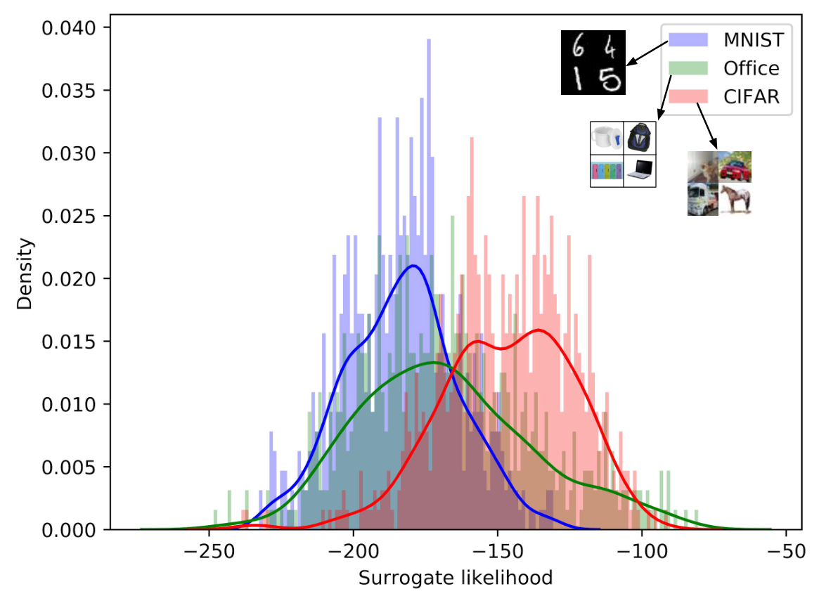
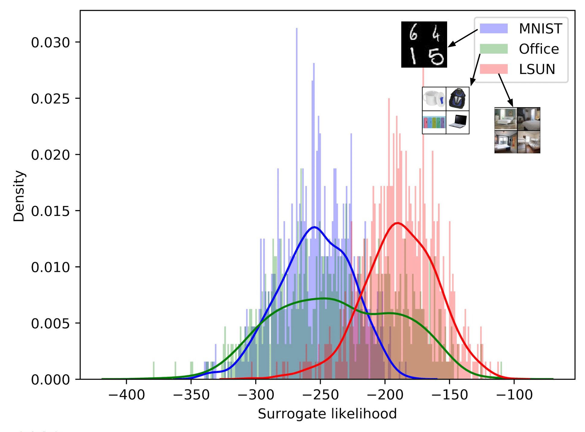
We use this approach to compute likelihood estimates for CIFAR-10 (Krizhevsky, 2009) and LSUN-Bedrooms (Yu et al., 2015) datasets. For CIFAR-10, we train DCGAN while for LSUN, we train WGAN. Fig. 4(a) demonstrates sample likelihood estimates of different datasets using a GAN trained on CIFAR-10. Likelihoods assigned to samples from MNIST and Office datasets are lower than that of the CIFAR dataset. Samples from the Office dataset, however, are assigned to higher likelihood values than MNIST samples. We note that the Office dataset is indeed more similar to the CIFAR dataset than MNIST. A similar experiment has been repeated for LSUN-Bedrooms (Yu et al., 2015) dataset. We observe similar performance trends in this experiment (Fig. 4(b)).
Appendix E Training Entropic GANs
In this section, we discuss how WGANs with entropic regularization is trained. As discussed in Section 3 (main paper), the dual of the entropic GAN formulation can be written as
where
We can optimize this min-max problem using alternating optimization. A better approach would be to take into account the smoothness introduced in the problem due to the entropic regularizer, and solve the generator problem to stationarity using first-order methods. Please refer to (Sanjabi et al., 2018) for more details. In all our experiments, we use Algorithm 1 of (Sanjabi et al., 2018) to train our GAN model.
E.1 GAN’s Training on MNIST
MNIST dataset constains grayscale images. As a pre-processing step, all images were resized in the range . The Discriminator and the Generator architectures used in our experiments are given in Tables. 3,4. Note that the dual formulation of GANs employ two discriminators - and , and we use the same architecture for both. The hyperparameter details are given in Table 5. Some sample generations are shown in Fig. 5
| Layer | Output size | Filters |
|---|---|---|
| Input | - | |
| Fully connected | ||
| Reshape | - | |
| BatchNorm+ReLU | - | |
| Deconv2d (, str ) | ||
| BatchNorm+ReLU | - | |
| Remove border row and col. | - | |
| Deconv2d (, str ) | ||
| BatchNorm+ReLU | - | |
| Deconv2d (, str ) | ||
| Sigmoid | - |
| Layer | Output size | Filters |
|---|---|---|
| Input | - | |
| Conv2D(, str ) | ||
| LeakyReLU() | - | |
| Conv2D(, str ) | ||
| LeakyReLU() | - | |
| Conv2d (, str ) | ||
| LeakyRelU() | - | |
| Reshape | - | |
| Fully connected |
| Parameter | Config |
|---|---|
| Generator learning rate | |
| Discriminator learning rate | |
| Batch size | |
| Optimizer | Adam |
| Optimizer params | , |
| Number of critic iters / gen iter | 5 |
| Number of training iterations | 10000 |


E.2 GAN’s Training on CIFAR
We trained a DCGAN model on CIFAR dataset using the discriminator and generator architecture used in (Radford et al., 2015). The hyperparamer details are mentioned in Table. 6. Some sample generations are provided in Figure 7
E.3 GAN’s Training on LSUN-Bedrooms dataset
We trained a WGAN model on LSUN-Bedrooms dataset with DCGAN architectures for generator and discriminator networks (Arjovsky et al., 2017). The hyperparameter details are given in Table. 7, and some sample generations are provided in Fig. 8
| Parameter | Config |
|---|---|
| Generator learning rate | |
| Discriminator learning rate | |
| Batch size | |
| Optimizer | Adam |
| Optimizer params | , |
| Number of training epochs | 100 |

| Parameter | Config |
|---|---|
| Generator learning rate | |
| Discriminator learning rate | |
| Clipping parameter | 0.01 |
| Number of critic iters per gen iter | 5 |
| Batch size | |
| Optimizer | RMSProp |
| Number of training iterations | 70000 |
