Conformal embeddings of $S^{2}\to\mathbb{R}^{3}$ with prescribed mean curvature: A variational approach

One of the fundamental topics in classical differential geometry concerns the question of whether a smooth Riemannian manifold can be isometrically immersed/embedded into Euclidean spaces. It has been conjectured by Schläfli in 1873 that every $m$-dimensional smooth Riemannian manifold $(M^{m},\textit{g})$ admits a local isometric embedding into $\mathbb{R}^{N_{m}}$, with $N_{m}=\frac{m(m+1)}{2}$. Several important achievements have been made towards this problem in the last century. In one of his outstanding papers, J. Nash [31] showed the existence of a global isometric embedding of any $m$-dimensional smooth Riemannian manifold in $\mathbb{R}^{N}$ with $N=3N_{m}+4m$ in the case of compact $M$ and $N=(m+1)(3N_{m}+4m)$ in the case of non-compact $M$. Following Nash, we mention the book ”Partial Differential Relations” published in 1986 by Gromov, which contains various problems related to the isometric embedding of Riemannian manifolds. Furthermore, in this book, Gromov showed that $N=N_{m}+2m+3$ is enough for the compact case.

In low dimensions, if one asks the more specific question of whether a given $2$-dimensional Riemann surface can be isometrically immersed/embedded into Euclidean $3$-space, not too much is known. Besides some general local existence results (see for example [34, 29] for real analytic metrics and for smooth metrics under suitable curvature assumptions), non-existence results seem to be easier to come by: for instance, Hilbert’s classical result that the hyperbolic plane does not admit an isometric immersion into $\mathbb{R}^{3}$, and the fact that a compact non-positively curved Riemann surface cannot be isometrically immersed into $\mathbb{R}^{3}$.

In the classical differential geometry of surfaces, the Gauß-Codazzi-Mainardi equations consist of a pair of related equations, and it incorporates the extrinsic curvature (or mean curvature) of the surface. The equations are precisely the integrability conditions to obtain an immersed surface in $\mathbb{R}^{3}$ (locally or on a simply connected domain). With the development of Spin Geometry and the theory of Dirac operators, an equivalent albeit simpler expression becomes well-known, namely the existence of a special spinor field called generalized Killing spinor field (see for instance [26, 33, 37, 38, 39] and references therein). This expression is the so-called spinorial Weierstraß representation, and can be understood as a geometrically invariant way for the representation of surfaces in Euclidean $3$-space.

In late 1990s, T. Friedrich has written a very nice article in which the spinorial Weierstraß representation is beautifully explained, see [17, Theorem 13]. Eventually, it turns out that there exists a one-to-one correspondence between the existence of an isometric immersion $(\widetilde{M}^{2},\textit{g})\hookrightarrow(\mathbb{R}^{3},\textit{g}_{\mathbb{R}^{3}})$ with mean curvature $H$ and the existence of a spinor field $\varphi$ with constant length satisfying the following Dirac equation

where $\widetilde{M}^{2}$ is the universal covering of $M^{2}$, $D_{\textit{g}}$ and $|\cdot|_{\textit{g}}$ are respectively the Dirac operator and the hermitian metric on the spinor bundle $\mathbb{S}(M^{2})$ over $(M^{2},\textit{g})$.

Following this idea, the situation is much clearer for simply connected surfaces. And one may naturally ask the following question:

It seems interesting to see that Question 2 can be investigated via a conformal change of Eq. (1.1). That is, we may begin with the standard Riemann sphere $(S^{2},\textit{g}_{S^{2}})$ and consider the following nonlinear partial differential equation involving the Dirac operator $D_{\textit{g}_{S^{2}}}$:

Suppose we have a spinor field $\psi$ that satisfies Eq. (1.2) and that never vanishes. Then one may introduce a conformal metric $\textit{g}=|\psi|_{\textit{g}_{S^{2}}}^{4}\textit{g}_{S^{2}}$ on $S^{2}$. Through the well-known formula for the Dirac operator under a conformal change of the metrics (see for instance [19, Proposition 1.3.10] and Proposition 2.1 below), we obtain a new spinor field $\varphi:=\iota(|\psi|_{\textit{g}_{S^{2}}}^{-1}\psi)$ which satisfies

where $\iota:(\mathbb{S}(S^{2}),\textit{g}_{S^{2}})\to(\mathbb{S}(S^{2}),\textit{g})$ is a fiberwise isometry. And thus we find an isometric immersion $(S^{2},\textit{g})\hookrightarrow(\mathbb{R}^{3},\textit{g}_{\mathbb{R}^{3}})$ that realizes $H$ as prescribed mean curvature.

In this paper, we will make use of the above spinorial tool in the study of Question 2. From this point of view, it seems natural to consider a two-step procedure:

• •

  find a non-trivial spinor field $\psi$ satisfying Eq. (1.2),

• •

  show that the zero set under $|\psi|_{\textit{g}_{S^{2}}}:S^{2}\to[0,\infty)$ is empty, i.e. $\psi^{-1}(0)=\emptyset$.

However this is not an easy task. In general, even if one already knows there exists a non-trivial solution $\psi$ to Eq. (1.2), it is still difficult to know whether $\psi$ possesses zeros. This is due to the lack of an adequate replacement for the maximum principle developed for second order elliptic partial differential operators.

Let us return to the problem of finding isometric immersions/embeddings of surfaces. The spinorial Weierstraß representation has transformed the problem into the equivalent problem which amount to solve a PDE on the spinor bundle over the surface. However, still, the picture is not completely clear for immersed surfaces. A further question besides Question 1 and 2 is the following:

In this paper, we are interested in answering Questions 1-3. In order to explain our results in more detail, we begin with the following theorem, which provides a description of the zero set (or nodal set) of a solution to (1.2).

After having studied the zero set, we discuss the existence of a (weak) solution to (1.3) on the $2$-sphere in the next theorem. In order to state the result, we introduce the following notation: For a function $H\in C^{2}(S^{2})$, we set $H_{max}:=\max_{\xi\in S^{2}}H(\xi)$ and $H_{min}:=\min_{\xi\in S^{2}}H(\xi)$. We then denote the set of maximum points as $\mathcal{H}:=\big\{\xi\in S^{2}:\,H(\xi)=H_{max}\big\}$, and $\mathcal{H}_{\delta}:=\big\{\xi\in S^{2}:\,\dist_{\textit{g}_{S^{2}}}(\xi,\mathcal{H})<\delta\big\}$ its $\delta$-neighborhood for $\delta>0$.

Our criteria of the function $H$ will be formulated as

• $(H)$

  $\mathcal{H}$ is not contractible in its $\delta$-neighborhood $\mathcal{H}_{\delta}$, for some small $\delta>0$, but there exits $d\in\big(\max\big\{\frac{1}{2}H_{max},\,H_{min}\big\},H_{max}\big)$ such that $\mathcal{H}$ is contractible in $\big\{\xi\in S^{2}:\,H(\xi)\geq d\big\}$. There is no critical value of $H$ in the interval $(d,H_{max})$, and if $\xi\in S^{2}$ is a critical point of $H$ with $H(\xi)=d$ then the Hessian of $H$ at $\xi$ is positive definite.

And then, combining Theorem 1.1, the result is as follows

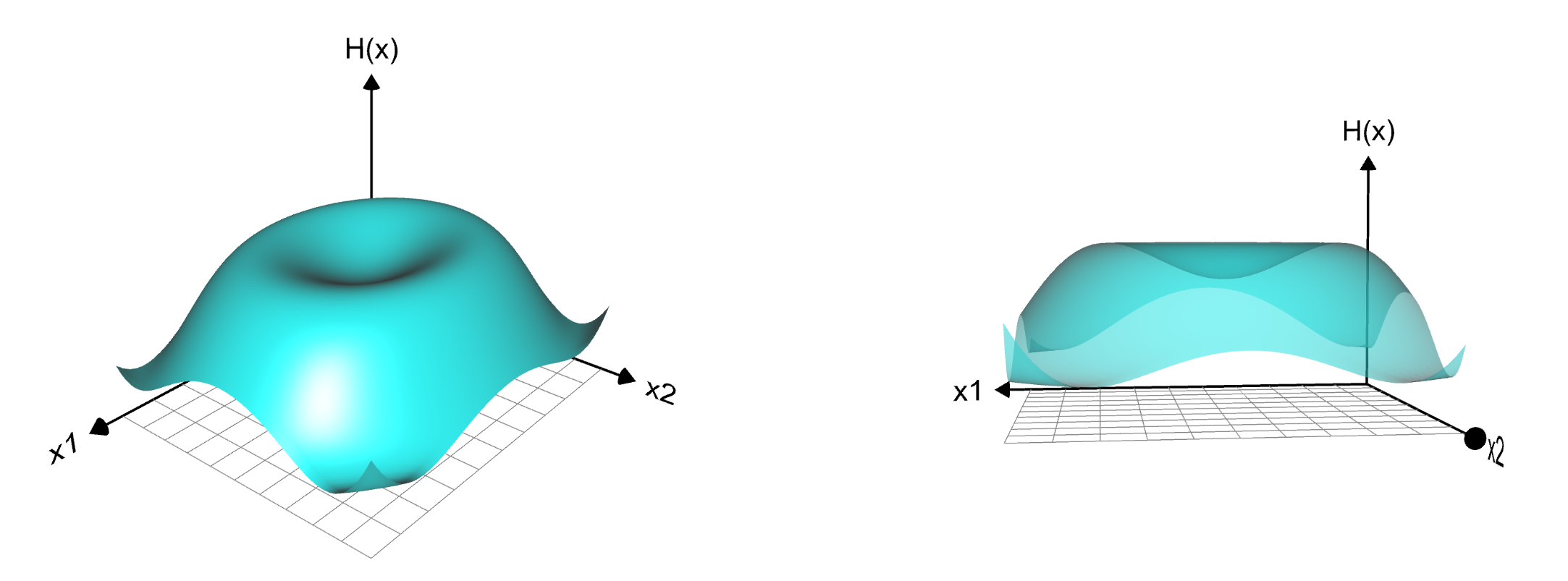
We note that the class of functions $H$ that satisfy the hypothesis $(H)$ is dense, in $C^{1}$-topology, in the space of positive smooth functions. Then Theorem 1.3 and Remark 1.4 together immediately imply the next corollary, which provides an answer to Question 1-3. For ease of notation, we will denote $[\textit{g}_{S^{2}}]=\big\{f^{2}\textit{g}_{S^{2}}:\,f\in C^{\infty}(S^{2}),f>0\big\}$ the standard conformal class of $\textit{g}_{S^{2}}$.

We point out that, in [24], T. Isobe also considered the Question 1 and 2. He proved that when the function $H$ is very close to a constant, that is $H(\xi)=1+\varepsilon Q(\xi)$ on $S^{2}$ with $Q$ being a specific Morse function and $\varepsilon>0$ is small, then there exists a branched immersion $\Pi_{\varepsilon,Q}:S^{2}\to\mathbb{R}^{3}$ that realizes its mean curvature as $1+\varepsilon Q$. Here, by branched immersion we mean that $\Pi_{\varepsilon,Q}$ is an immersion except at a discrete set of points. The method in [24] is also based on the spinorial Weierstraß representation and the nonlinear Dirac equation (1.2).

Another result concerning this problem is due to M. Anderson [8]. He proved that for any positive function $H:S^{2}\to(0,\infty)$ in the class $C^{k,\alpha}$, $k\geq 0$ and $\alpha\in(0,1)$, there exists a branched immersion $\Pi:S^{2}\to\mathbb{R}^{3}$ and an positive affine function $\ell$ on $S^{2}$ such that the mean curvature of $\Pi$ is prescribed by $H+\ell$. In this setting the function $H>0$ lies arbitrarily in the class $C^{k,\alpha}$, and thus it can be far away from a constant. However, the affine function $\ell$ cannot be prescribed.

Note that, in Corollary 1.5, the mean curvature is accurately prescribed by the functions in the class $\mathscr{H}$ and, particularly, the presence of branch points is ruled out. Hence, comparing with [24, 8], our approach is in a different perspective. The class $\mathscr{H}$ has its generality in the sense that only a ”volcano”-shaped assumption is required and, furthermore, such a class of functions can give an explicit estimate of the Willmore functional from above. However, Corollary 1.5 can not cover any of the results in [24, 8] but has intersection with them. There are many functions lying outside $\mathscr{H}$ that can be prescribed as mean curvature of certain conformal isometric embeddings. However, there are still several problems that have to be solved.

Last but not least, we want to remind the readers that Eq. (1.2) for an arbitrarily given $H$ does not necessarily admit a non-trivial solution. As was shown in [7], there is an obstruction to the existence of a non-trivial solution to Eq. (1.2). In fact, if there exists a non-trivial solution $\psi$ to Eq. (1.2), then $H$ must satisfy

for any conformal vector field $X$ on $S^{2}$. In particular, $\nabla_{X}H$ must change sign on $S^{2}$. The obstruction (1.5) is quite similar to the Kazdan-Warner obstruction for Gaussian and scalar curvature equations (see [25]).

Let us give an overview of our paper as follows. We will consider the following semilinear Dirac equation with a critical exponent in all dimensions:

under the generalized assumption that $H\in C^{2}(S^{m})$ satisfies

• $(H*)$

  $\mathcal{H}$ is not contractible in its $\delta$-neighborhood $\mathcal{H}_{\delta}$, for some small $\delta>0$, but there exits $d\in\big(\max\big\{2^{-\frac{1}{m-1}}H_{max},\,H_{min}\big\},H_{max}\big)$ such that $\mathcal{H}$ is contractible in $\big\{\xi\in S^{m}:\,H(\xi)\geq d\big\}$. There is no critical value of $H$ in the interval $(d,H_{max})$, and if $\xi\in S^{m}$ is a critical point of $H$ with $H(\xi)=d$ then the Hessian of $H$ at $\xi$ is positive definite.

Here, analogous to the $2$-sphere case, $H_{max}:=\max_{\xi\in S^{m}}H(\xi)$ and $H_{min}:=\min_{\xi\in S^{m}}H(\xi)$, $\mathcal{H}:=\big\{\xi\in S^{m}:\,H(\xi)=H_{max}\big\}$ is the collection of maximum points and $\mathcal{H}_{\delta}:=\big\{\xi\in S^{m}:\,\dist_{\textit{g}_{S^{m}}}(\xi,\mathcal{H})<\delta\big\}$ is its $\delta$-neighborhood for $\delta>0$. Inspired by the idea of Yamabe [44] and Aubin [9] when they deal with the Yamabe problem, here we mainly focus on a specific regularization of Eq. (1.6), namely, a family of related equations with subcritical exponent

where $p\in(2,\frac{2m}{m-1})$. If one considers the variational formulation where solutions of Eq. (1.7) are obtained as critical points of the energy functional

then the main ingredient of this paper lies in the compactness of a family of critical points $\psi_{p}$ as $p\to\frac{2m}{m-1}$ of $\mathcal{L}_{p}$. One way to show the compactness is to apply the regularity arguments to get uniform $C^{1,\alpha}$-boundedness for $\psi_{p}$, and hence by Arzelà-Ascoli theorem, up to a subsequence, the spinor field $\psi_{p}$ converges to a solution of Eq. (1.6). This has been shown when the energy $\mathcal{L}_{p}(\psi_{p})$ is below a so-called blow-up threshold (see [4, 32]). However, in our case, one must allow for blow-up phenomenon, and the situation becomes much more complicated. Whether or not one can obtain a uniform $C^{1,\alpha}$-boundedness for these $\psi_{p}$ is not clear. Here our strategy is to use build a concentration-compactness alternative for the sequence $\{\psi_{p}\}$. To rule out the blow-up phenomenon, one only needs to clarify that concentration will not occur, and this will be done in Section 4.

From the view point of variational calculus, there are at least three different kinds of analytical difficulties when carrying out the above program. The first one is due to the strong indefiniteness of the functional $\mathcal{L}_{p}$. It is well-known that the spectrum of the Dirac operator $D_{\textit{g}_{S^{m}}}$ is neither bounded from above nor from below. Hence, a critical point of $\mathcal{L}_{p}$ has infinite Morse index and infinite co-index. This will cause a problem since the classical variational methods such as the minimizing technique, Morse theory and its variants do not directly apply. The second difficulty is due to the existence of multiple solutions to the subcritical equation (1.7). Note that Eq. (1.7) is invariant under the canonical action of $S^{1}=\{e^{i\theta}\in\mathbb{C}:\,\theta\in[0,2\pi]\}$ on spinors (i.e. if $\psi$ is a solution of Eq. (1.7) then $e^{i\theta}\psi$ is also a solution, for every fixed $\theta$). Moreover, for the case $m\equiv 2,3,4$ (mod $8$), the spinor bundle has a quaternionic structure which commutes with Clifford multiplication, see for instance the construction in [18, Section 1.7] or [27, Page 33, Table III]. Thus in these cases, Eq. (1.7) is invariant under the canonical action of the unit quaternions $S^{3}=\{q\in\mathbb{H}:\,|q|=1\}$ on spinors. And then one may be interested in the existence of $\mathcal{G}$-inequivalent solutions of Eq. (1.7), where $\mathcal{G}=S^{1}$ or $S^{3}$. Standard variational arguments (see e.g. [35, Chapter 2 Section 5]) show that the symmetric property of Eq. (1.7) under $\mathcal{G}$-actions ensures multiple $\mathcal{G}$-orbits of solutions. It can be seen from Remark 2.9 that, among all these $\mathcal{G}$-orbits of solutions, the ground state energy solutions should blow up when $p\to\frac{2m}{m-1}$. Whether or not there exists a sequence of solutions $\{\psi_{p}\}$ which shows compactness when $p$ approaches to $\frac{2m}{m-1}$ becomes a problem. Another difficulty lies in the analysis of the zero sets for a solution to Eq. (1.6). Since the equation is defined on the spinor bundle, which is a complex vector bundle, in contrast to the Laplacian on functions, we do not have a maximum principle in order to exclude zeros for eigenspinors.

In what follows, the proof will be carried out as follows: in Section 2, we introduce some notation and recall some known facts about the Dirac operator and blow-up asymptotic behavior of Eq. (1.7); the analysis of zero sets for a solution to (1.6) on surfaces will be given in Section 3; the detailed proof of Theorem 1.3 and Corollary 1.5 are given in Section  4.

References

- [2] R. Adams, Sobolev Spaces, Academic Press, New York, (1975).
- [3] A. D. Alexandrov, Uniqueness theorems for surfaces in the large, Amer. Math. Soc. Transl. Ser. 2, 21, 441-519, (1962).
- [4] B. Ammann, A variational problem in conformal spin geometry, Habilitationsschift, Universität Hamburg, (2003).
- [5] B. Ammann, The smallest Dirac eigenvalue in a spin-conformal class and cmc immersions, Comm. Anal. Geom. 17 (2009), no. 3, 429-479.
- [6] B. Ammann, J.-F. Grossjean, E. Humbert, B. Morel, A spinorial analogue of Aubin’s inequality, Math. Z. 260 (2008), 127-151.
- [7] B. Ammann, E. Humbert, M. Ould. Ahmedou, An obstruction for the mean curvature of a conformal immersion , Proc. Amer. Math. Soc. 135 (2007), no. 2, 489-493.
- [8] M. Anderson, Conformal immersions of prescribed mean curvature in , Nonlinear Anal. 114 (2015), 142-157.
- [9] T. Aubin, Équations différentielles non linéaires et problème de Yamabe concernant la courbure scalaire, J. Math. Pures Appl. 55 (1976), 269-296.
- [10] C. Bär, On nodal sets for Dirac and Laplace operators, Comm. Math. Phys. 188 (1997), 709-721.
- [11] T. Bartsch, T. Xu, A spinorial analogue of the Brezis-Nirenberg theorem involving the critical Sobolev exponent, J. Funct. Anal. 280 (2021), 108991.
- [12] B. Booss-Bavnbek, M. Marcolli, B.L. Wang, Weak UCP and perturbed monopole equations, Int. J. Math. 13, 987 (2002).
- [13] J.-P. Bourguignon, P. Gauduchon, Spineurs, opérateurs de Dirac et variations de métriques, Comm. Math. Phys. 144 (1992), no. 3, 581-599.
- [14] B. Buffoni, L. Jeanjean, C.A. Stuart, Existence of a non-trivial solution to a strongly indefinite semilinear equation, Proc. Amer. Math. Soc., 119 (1993), 179-186.
- [15] Q. Chen, J. Jost, G. Wang, Nonlinear Dirac equations on Riemann surfaces, Ann. Global Anal. Geom. 33 (2008), 253-270.
- [16] I. Ekeland, On the variational principle, J. Math. Anal. Appl. 47 (1974), 324-353.
- [17] T. Friedrich, On the spinor representation of surfaces in Euclidean -space, J. Geom. Phys. 28 (1998), no. 1-2, 143-157.
- [18] T. Friedrich, Dirac Operators in Riemannian Geometry, Grad. Stud. Math., vol 25, Amer. Math. Soc., Providence (2000).
- [19] N. Ginoux, The Dirac Spectrum, Lecture Notes in Mathematics, vol. 1976. Springer, Berlin (2009).
- [20] O. Hijazi, A conformal lower bound for the smallest eigenvalue of the Dirac operator and Killing spinors, Comm. Math. Phys. 104 (1986), 151-162.
- [21] N. Hitchin, Harmonic spinors, Adv. Math. 14 (1974), 1-55.
- [22] W-Y. Hsiang, Z-H. Teng, W-C. Yu, New examples of constant mean curvature immersions of -spheres into Euclidean -Space, Ann. of Math., 117 (1983), 609-625.
- [23] T. Isobe, Nonlinear Dirac equations with critical nonlinearities on compact Spin manifolds, J. Funct. Anal. 260 (2011), no. 1, 253-307.
- [24] T. Isobe, A perturbation method for spinorial Yamabe type equations on and its application, Math. Ann. 355 (2013), no. 4, 1255-1299.
- [25] J. Kazdan, F. Warner, Existence and conformal deformation of metrics with prescribed Gaussian and scalar curvature, Ann. Math. 101 (1975), 317-331.
- [26] R. Kusner, N. Schmitt, Representation of surfaces in space, arXiv:dg-ga/9610005, (1996).
- [27] H.B. Lawson, M.L. Michelson, Spin Geometry, Princeton University Press (1989).
- [28] P. Li, S.T. Yau, A new conformal invariant and its applications to the Willmore conjecture and the first eigenvalue on compact surfaces, Invent. Math. 69 (1982), 269-291.
- [29] C. S. Lin, The local isometric embedding in of two-dimensional Riemannian manifolds with gaussian curvature changing sign cleanly, Comm. Pure Applied Math., 39.6 (1986), 867-887.
- [30] J. Mawhin, M. Willem, Critical Point Theory and Hamiltonian Systems, Springer-Verlag, New York, 1989.
- [31] J. Nash, The Imbedding Problem for Riemannian Manifolds, Ann. of Math., 63, no. 1 (1956), 20-63.
- [32] S. Raulot, A Sobolev-like inequality for the Dirac operator, J. Funct. Anal. 256 (2009), 1588-1617.
- [33] J. Roth, Spinorial characterizations of surfaces into 3-homogeneous manifolds, J. Geom. Phys., 60 (2010), 1045-1061.
- [34] M.D. Spivak, A comprehensive introduction to differential geometry, Publish or perish, 1970.
- [35] M. Struwe, Variational methods, Springer-Verlag, Berlin, 2008.
- [36] S. Sulanke, Die Berechnung des Spektrums des Quadrates des Dirac-Operators auf der Sphäre, Doktorarbeit. Humboldt-Universität zu Berlin, Berlin, 1979.
- [37] I.A. Taimanov, Surfaces of revolution in terms of solitons, Ann. Global Anal. Geom. 15 (1997), no. 5, 419-435.
- [38] I.A. Taimanov, Modified Novikov-Veselov equation and differential geometry of surfaces, Amer. Math. Soc. Transl. Ser. 2, 179 (1997) 133-151.
- [39] I.A. Taimanov, The Weierstrass representation of closed surfaces in , Funct. Anal. Appl. 32 (1998), no. 4, 258-267.
- [40] C.Y. Wang, A remark on nonlinear Dirac equations, Proc. Amer. Math. Soc. 138 (2010), no. 10, 3753-3758.
- [41] M. Willem, Minimax Theorems, Birkhäuser, 1996.
- [42] T.J. Willmore, Note on embedded surfaces, An. Sti. Univ. ”Al. I. Cuza” Iasi Sect. I a Mat. (N.S.) 11B (1965), 493-496.
- [43] T.J. Willmore, Riemannian Geometry, Oxford Science Publications. Oxford University Press, 1993.
- [44] H. Yamabe, On the deformation of Riemannian structures on compact manifolds, Osaka Math. J. 12 (1960) 21-37.
Tian Xu
Center for Applied Mathematics, Tianjin University
Tianjin, 300072, China
xutian@amss.ac.cn