A Three-Dimensional Hybrid Spectral Element-Fourier Spectral Method for Wall-Bounded Two-Phase Flows

S.H. Challa S. Dong ^†^†thanks: Author of correspondence. Email: sdong@purdue.edu Affiliation: Department of MathematicsPurdue UniversityWest Lafayette, Indiana, USA L.D. Zhu Affiliation: Department of MathematicsIndiana University-Purdue University IndianapolisIndianapolis, Indiana, USA [0.1in] School of Aeronautics Astronautics

Abstract

We present a hybrid spectral element-Fourier spectral method for solving the coupled system of Navier-Stokes and Cahn-Hilliard equations to simulate wall-bounded two-phase flows in a three-dimensional domain which is homogeneous in at least one direction. Fourier spectral expansions are employed along the homogeneous direction and $C^{0}$ high-order spectral element expansions are employed in the other directions. A critical component of the method is a strategy we developed in a previous work for dealing with the variable density/viscosity of the two-phase mixture, which makes the efficient use of Fourier expansions in the current work possible for two-phase flows with different densities and viscosities for the two fluids. The attractive feature of the presented method lies in that the two-phase computations in the three-dimensional space are transformed into a set of de-coupled two-dimensional computations in the planes of the non-homogeneous directions. The overall scheme consists of solving a set of de-coupled two-dimensional equations for the flow and phase-field variables in these planes. The linear algebraic systems for these two-dimensional equations have constant coefficient matrices that need to be computed only once and can be pre-computed. We present ample numerical simulations for different cases to demonstrate the accuracy and capability of the presented method in simulating the class of two-phase problems involving solid walls and moving contact lines.

Key words: hybrid discretization; two-phase flow; contact angle; Fourier spectral method; spectral element method; wall-bounded flow

1 Introduction

This work focuses on three-dimensional (3D) incompressible two-phase flows, comprised of two immiscible incompressible fluids with different densities and viscosities, on flow domains which are homogeneous in at least one direction and can be arbitrarily complex in the other directions. By “homogeneous in one direction” we mean that the 3D domain is an extrusion of a two-dimensional (2D) domain in the third (homogeneous) direction and it is infinite along that direction. While seemingly a little restrictive with the homogeneity requirement, this class of problems encompasses a wide range of important two-phase flows such as those in the pipes, channels, boundary layers, shear layers, and the two-phase flows past long bluff bodies (e.g. cylinders with cross sections of various shapes), to name just a few. It should be noted that flows in such domains are in general three-dimensional, except at low Reynolds numbers with certain flow configurations. For example, for the single-phase flow past an infinitely long circular cylinder, the cylinder wake is two-dimensional at Reynolds numbers below about $185$ and it transitions to a three-dimensional flow for Reynolds numbers beyond about $260$ [34]. In the current work we assume that in the non-homogeneous directions the domain may be bounded by solid walls with certain wetting properties. It is further assumed that the two-phase system consists of two immiscible incompressible fluid components, which can be liquid/liquid or liquid/gas, and no solid phase (e.g. solid particles) is involved except solid-wall boundaries.

This class of 3D two-phase problems can potentially allow the use of fast Fourier transforms (FFT) along the homogeneous direction. One can then transform the 3D problem into a set of weakly-coupled or un-coupled 2D problems about the Fourier modes on the discrete level. The 3D computations can be reformulated into the solution of a series of 2D problems, which can be performed largely in parallel. This will enable very efficient simulations of 3D two-phase flows. This idea motivates the current work.

Applying this idea to two-phase flows with generally different densities and viscosities for the two fluids, one immediately encounters difficulties. The predominant difficulty lies in the field-dependent variable fluid properties (e.g. mixture density and viscosity), which would give rise to differential equations in space with variable coefficients upon temporal discretization. Performing FFT thus induces convolutions with the coefficient functions in the frequency space, which couples together all the Fourier modes of the unknown flow variable to be solved for and completely defeats the purpose for using FFTs. This situation is very different from single-phase flows (see e.g. [24, 14, 8, 16]) and two-phase problems with matched densities and viscosities for the two fluids (see e.g. [22, 35]), in which the fluid properties are all constant and cause no difficulty when Fourier transforms and expansions are used. Note that the energy-stable type schemes (see e.g. [30, 31, 2, 17], among others) are not suitable with FFT because they give rise to differential equations in space with variable coefficients even with matched fluid properties for the two fluids and with constant fluid properties for the two-phase mixture.

This difficulty can be circumvented. In [15] we have developed a strategy to deal with the variable density and variable viscosity for two-phase problems in two dimensions. The main idea lies in reformulations of the pressure and viscous terms in the momentum equation as follows,

\left\{\begin{split}&\frac{1}{\rho}\nabla p\approx\frac{1}{\rho_{0}}\nabla p+\left(\frac{1}{\rho}-\frac{1}{\rho_{0}}\right)\nabla p^{*}\\ &\frac{\mu}{\rho}\nabla^{2}\mathbf{u}\approx\nu_{m}\nabla^{2}\mathbf{u}-\left(\frac{\mu}{\rho}-\nu_{m}\right)\nabla\times\nabla\times\mathbf{u}^{*},\end{split}\right.

(1)

where $\rho$ and $\mu$ are the variable density and dynamic viscosity of the mixture (field functions), $\rho_{0}$ and $\nu_{m}$ are two appropriate constants, $p$ and $\mathbf{u}$ are the pressure and velocity to be computed, and $p^{*}$ and $\mathbf{u}^{*}$ are the pressure and velocity that are approximated explicitly with a prescribed order of accuracy in time. The second approximation in the above has employed the velocity divergence-free property ( $\nabla\cdot\mathbf{u}=0$ ). These approximations essentially incorporate certain zero terms, such as $\frac{1}{\rho_{0}}\nabla(p-p^{*})$ , which are equivalent to zero to the prescribed order of accuracy. They can lead to differential equations in space with constant coefficients upon temporal discretization, and make the efficient use of FFTs possible for two-phase flows with different densities and viscosities for the two fluids. This strategy is critical to the developments in the current work.

The approach taken in this work for dealing with two phases and fluid interfaces falls into the phase field framework. Phase field is one of the often-used approaches for two-phase problems [3, 23, 18, 22, 35]. We refer the reader to the reviews [26, 29, 33, 28] and the references therein for related approaches such as level set, volume of fluids, and front tracking. With the phase field approach, the fluid interface is treated as a diffuse interface (thin transition layer), and regions of different fluids are marked by the phase field function. The phase field function varies smoothly over the diffuse interfacial layer and is mostly uniform in the bulk of the fluids. The evolution of the system is described by the system of the Navier-Stokes equations and the Cahn-Hilliard equation, which stems from the mass balance relation of the system [1, 10].

The increasing popularity of phase field method for two-phase flows in recent years is due to the contributions of many researchers (see e.g. [3, 23, 19, 22, 4, 35, 7, 1, 15, 21, 11], among others). Phase field is a physics-based approach [13]. The effect of surface tension in the two-phase system is characterized by the free energy density function. Certain component terms in the free energy density promote the mixing of the two fluids, while the other terms tend to segregate different fluids. The interplay of these two tendencies determines the profile of the interface. This method can deal with contact lines and contact angles relatively easily due to the diffuse interface [19, 27, 36, 9], which is a prominent feature when compared with other related methods. The contact angle on the solid wall can be enforced by imposing appropriate boundary conditions. Since the phase field Cahn-Hilliard equation is of fourth order in space, two independent boundary conditions are required on the wall boundary. One boundary condition can be used to enforce the mass conservation, and the other condition can be used to impose the contact angle at the wall [19, 36, 9, 12]. Only the static (equilibrium) contact angle will be considered in the current paper. We refer to e.g. [9, 5] for discussions of the effect of dynamic contact angles in the literature.

In this paper we present an efficient hybrid spectral element-Fourier spectral method for wall-bounded two-phase flows on 3D domains with at least one homogeneous direction. Fourier expansions of the field variables are performed along the homogeneous direction, and the difficulty caused by the variable density/viscosity of the two-phase mixture is overcome by exploiting the strategy represented by equation (1). This allows the efficient simulations of 3D two-phase flows with different densities and dynamics viscosities for the two fluids. In the plane of the non-homogeneous directions high-order $C^{0}$ spectral elements are employed, which can allow us to deal with domains with complex geometry in those directions. The presented method has the advantage that the two-phase computations in 3D space are decomposed into a set of problems for the Fourier modes in the 2D planes, which are completely de-coupled from one another. The method provides an efficient technique for simulating 3D two-phase flows.

The rest of this paper is organized as follows. In Section 2, we discuss how to discretize the governing equations and boundary conditions for incompressible two-phase flows with the hybrid Fourier spectral and spectral element method. In Section 3 we present extensive numerical examples of 3D two-phase problems to test the convergence rates, accuracy and performance of the method developed herein. Section 4 concludes the discussions with some closing remarks.

2 Hybrid Spectral Element-Fourier Spectral Method

2.1 Flow Domain, Governing Equations, and Boundary Conditions

We consider the dynamics of two incompressible immiscible fluids contained in a flow domain in the three-dimensional (3D) space. In the present work we concentrate on the class of problems with the flow domain having the following property:

•

The domain is homogeneous in at least one direction (denoted as $z$ direction), while in the other two ( $x$ and $y$ ) directions it can be arbitrarily complex.

As such, a Fourier spectral expansion of the field variables can be performed along the homogeneous direction to take advantage of the fast Fourier transforms (FFT), and spectral element expansions of the field variables can be performed within the $x$ - $y$ planes to deal with the complex geometry.

To simulate this class of problems, we choose a computational domain with dimension $L_{z}$ along the homogeneous direction ( $0\leqslant z\leqslant L_{z}$ ), and assume that all the field variables and the domain are periodic at $z=0$ and $z=L_{z}$ . Let $\Omega$ denote the 3D computational domain, and $\partial\Omega$ denote the 3D domain boundary. Let $\Omega_{2D}$ denote the projection of the 3D domain onto the $x$ - $y$ plane, and $\partial\Omega_{2D}$ denote its boundary. Then we have

\Omega=\Omega_{2D}\otimes[0,L_{z}],\quad\partial\Omega=\partial\Omega_{2D}\otimes[0,L_{z}].

(2)

Let $\mathbf{n}$ denote the outward-pointing unit vector normal to $\partial\Omega$ , and $\mathbf{n}_{2D}$ denote the outward-pointing unit vector normal to $\partial\Omega_{2D}$ within the 2D $x$ - $y$ plane. It should be noted that $\mathbf{n}=(\mathbf{n}_{2D},0)$ , namely, $\mathbf{n}$ has zero component in the homogeneous direction.

Based on the phase-field approach, the dynamics of the flow is described by the following system of coupled Navier-Stokes and Cahn-Hilliard equations (see [22, 35, 15]),

	$\rho\left(\frac{\partial\textbf{u}}{\partial t}+\textbf{u}\cdot\nabla\textbf{u}\right)=-\nabla p+\nabla\cdot[\mu\textbf{D}(\textbf{u})]-\nabla\cdot(\lambda\nabla\phi\nabla\phi)+\textbf{f},$		(3a)
	$\nabla\cdot\textbf{u}=0$		(3b)
	$\frac{\partial\phi}{\partial t}+\textbf{u}\cdot\nabla\phi=-\lambda\gamma_{1}\nabla{{}^{2}}\left[\nabla{{}^{2}}\phi-h(\phi)\right]+g(\textbf{x,}t).$		(3c)

In the above equations, x and $t$ are the spatial coordinate and time, respectively. $\textbf{u}(\textbf{x,}t)$ is the velocity, and $p(\textbf{x,}t)$ is the pressure. $\textbf{D}(\textbf{u})=\nabla\textbf{u}+(\nabla\textbf{u}){{}^{T}}$ , where ( $\cdot$ )^T denotes the transpose of ( $\cdot$ ). $\textbf{f}(\textbf{x,}t)$ is an external body force. $\phi(\textbf{x,}t)$ is the phase field function, $-1\leq\phi\leq 1.$ The flow regions containing the first and second fluids are denoted by $\phi=1$ and $\phi=-1$ respectively, and the iso-surface $\phi(\textbf{x,}t)=0$ denotes the fluid interface at time $t$ . The function $h(\phi)$ in (3c) is given by, $h(\phi)=\frac{1}{\eta{}^{2}}\phi(\phi{{}^{2}}-1)$ , where $\eta$ is the characteristic length scale of the interface thickness. $\lambda$ is the mixing energy density coefficient, given by $\lambda=\frac{3}{2\sqrt{2}}\sigma\eta$ [35], where $\sigma$ is the surface tension (assumed to be constant). $\gamma_{1}$ denotes the mobility of the interface, and it is also assumed to be constant. The mixture density $\rho$ and dynamic viscosity $\mu$ are given by,

\rho(\phi)=\frac{\rho_{1}+\rho_{2}}{2}+\frac{\rho_{1}-\rho_{2}}{2}\phi,\quad\mu(\phi)=\frac{\mu_{1}+\mu_{2}}{2}+\frac{\mu_{1}-\mu_{2}}{2}\phi

(4)

where $\rho_{1}$ and $\rho_{2}$ are the constant densities of the two fluids, and $\mu_{1}$ and $\mu_{2}$ are the constant dynamic viscosities of the two fluids, respectively. Since $\phi$ is time-dependent, both $\rho(\phi)$ and $\mu(\phi)$ are field functions and vary in time. $g(\textbf{x,}t)$ in (3c) is a prescribed source term for the purpose of numerical testing only, and will be set to zero in practical simulations.

We assume that the flow domain is bounded in the non-homogeneous directions by solid walls with certain wetting properties. Correspondingly, the governing equations (3a)–(3c) are supplemented by the following boundary conditions:

	$\textbf{u}=\textbf{w}(\textbf{x,}t),\ \text{on}\ \partial\Omega$		(5a)
	$\textbf{n}\cdot\nabla[\nabla{{}^{2}}\phi-h(\phi)]=\textbf{g}_{c}(\textbf{x,}t),\ \text{on}\ \partial\Omega$		(5b)
	$\textbf{n}\cdot\nabla\phi+\frac{1}{\lambda}\textbf{f}^{\prime}_{w}(\phi)+\textbf{g}_{b}(\textbf{x,}t)=0,\ \text{on}\ \partial\Omega$		(5c)

where $\mathbf{w}$ is the boundary velocity, and $\textbf{g}_{b}(\textbf{x,}t)$ and $\textbf{g}_{c}(\textbf{x,}t)$ are prescribed source terms for numerical testing only and will be set to $g_{b}=0$ and $g_{c}=0$ in actual simulations. The boundary condition (5b) with $g_{c}=0$ enforces the mass conservation and the condition (5c) with $g_{b}=0$ enforces the static contact angle on the wall [9]. The function $f_{w}(\phi)$ represents the wall energy density, and $\textbf{f}^{\prime}_{w}(\phi)$ is given by (see [9]):

\textbf{f}^{\prime}_{w}(\phi)=-\frac{3}{4}\sigma(1-\phi^{2})\cos\theta_{s}.

(6)

where $\theta_{s}$ is the static contact angle formed between the solid wall and the fluid interface measured on the side of the first fluid. In the present work, only the effect of the static contact angle will be considered. One can refer to e.g. [9] for a study of the effect of dynamic contact angles.

Finally, the governing equations are supplemented by the initial conditions for the velocity and the phase field function as follows:

\textbf{u}(\textbf{x},0)=\textbf{u}_{in}(\textbf{x}),

(7)

\phi(\textbf{x},0)=\phi_{in}(\textbf{x}),

(8)

where $\mathbf{u}_{in}$ and $\phi_{in}$ are the initial velocity and phase field distributions.

2.2 Variable Density/Viscosity and the Difficulty Caused to Fourier Transform

Using Fourier spectral expansions to numerically solve the governing equations (3a)-(3c) together with the boundary conditions (5a)–(5c), one confronts an immediate difficulty. The difficulty is associated with the variable density $\rho(\phi)$ and variable viscosity $\mu(\phi)$ of the two-phase mixture, because these are field functions. A naive treatment of those terms involving these variables would lead to semi-discretized equations about the flow variables whose coefficients are field functions (not constants). Upon Fourier expansion, this will give rise to a convolution of the Fourier modes for the flow variable to be solved for and the Fourier modes of the coefficient function. Therefore, all the Fourier modes of the flow variable will be coupled together, which defeats the purpose for using Fourier transforms.

This difficulty associated with the variable density and variable viscosity can be circumvented. The key lies in a strategy we developed in [15] for two dimensions, by a reformulation of the pressure term and the viscous term as given in equation (1). We will exploit this strategy in the current work. This will enable the use of Fourier spectral expansions and efficient computations based on FFT.

We employ the following scheme for time stepping of the 3D two-phase governing equations, which is modified from that of [15] and incorporates the reformulations given in equation (1). By introducing an auxiliary pressure, $P=p+\frac{\lambda}{2}\nabla\phi\cdot\nabla\phi$ , equation (3a) can be transformed into

\frac{\partial\textbf{u}}{\partial t}+\textbf{u}\cdot\nabla\textbf{u}=-\frac{1}{\rho}\nabla P+\frac{\mu}{\rho}\nabla{{}^{2}}\textbf{u}+\frac{1}{\rho}\nabla\mu\cdot\mathbf{D}(\mathbf{u})-\frac{\lambda}{\rho}\left(\nabla{{}^{2}}\phi\right)\nabla\phi+\frac{1}{\rho}\mathbf{f}.

(9)

Let $n\geqslant 0$ denote the time step index and $(\cdot)^{n}$ denote the variable $(\cdot)$ at time step $n$ . Let $J$ ( $J=1$ or $2$ ) denote the temporal order of accuracy. Given $(\phi^{n},P^{n},\mathbf{u}^{n})$ , we solve $\phi^{n+1}$ , $P^{n+1}$ and $\mathbf{u}^{n+1}$ successively as follows.
For $\phi{{}^{n+1}}$ :

	$\frac{\gamma_{0}\phi^{n+1}-\hat{\phi}}{\Delta t}+\textbf{u}^{,n+1}\cdot\nabla\phi^{,n+1}=-\lambda\gamma_{1}\nabla^{2}\left[\nabla^{2}\phi^{n+1}-\frac{S}{\eta^{2}}\left(\phi^{n+1}-\phi^{,n+1}\right)-h(\phi^{,n+1})\right]+g^{n+1},$		(10a)
	$\textbf{n}\cdot\nabla\left[\nabla^{2}\phi^{n+1}-\frac{S}{\eta^{2}}(\phi^{n+1}-\phi^{,n+1})-h(\phi^{,n+1})\right]=g_{c}^{n+1},\quad\text{on}\ \partial\Omega,$		(10b)
	$\textbf{n}\cdot\nabla\phi^{n+1}=-\frac{1}{\lambda}f^{\prime}_{w}(\phi^{*,n+1})-g_{b}^{n+1},\quad\text{on}\ \partial\Omega.$		(10c)

For $P^{n+1}$ :

	$\frac{\gamma_{0}\tilde{\textbf{u}}^{{n+1}}-\hat{\textbf{u}}}{\Delta t}+\frac{1}{\rho_{0}}\nabla P^{n+1}=-\textbf{u}^{,n+1}\cdot\nabla\textbf{u}^{,n+1}+\left(\frac{1}{\rho_{0}}-\frac{1}{\rho^{n+1}}\right)\nabla P^{,n+1}-\frac{\mu^{n+1}}{\rho^{n+1}}\nabla\times\nabla\times\textbf{u}^{,n+1}\\ +\frac{1}{\rho^{n+1}}\nabla\mu^{n+1}\cdot\textbf{D}(\textbf{u}^{*,n+1})-\frac{\lambda}{\rho^{n+1}}\nabla^{2}\phi^{n+1}\nabla\phi^{n+1}+\frac{1}{\rho^{n+1}}\mathbf{f}^{n+1},$		(11a)
	$\nabla\cdot\tilde{\textbf{u}}^{n+1}=0,$		(11b)
	$\textbf{n}\cdot\tilde{\textbf{u}}^{n+1}=\textbf{n}\cdot\textbf{w}^{n+1},\quad\text{on}\ \partial\Omega$		(11c)

For $\textbf{u}^{n+1}$ :

	$\begin{split}\frac{\gamma_{0}\textbf{u}^{{n+1}}-\hat{\textbf{u}}}{\Delta t}&+\frac{1}{\rho_{0}}\nabla P^{n+1}-\nu_{m}\nabla^{2}\mathbf{u}^{n+1}=-\textbf{u}^{,n+1}\cdot\nabla\textbf{u}^{,n+1}+\left(\frac{1}{\rho_{0}}-\frac{1}{\rho^{n+1}}\right)\nabla P^{,n+1}\\ &+\left(\nu_{m}-\frac{\mu^{n+1}}{\rho^{n+1}}\right)\nabla\times\nabla\times\textbf{u}^{,n+1}+\frac{1}{\rho^{n+1}}\nabla\mu^{n+1}\cdot\textbf{D}(\textbf{u}^{*,n+1})\\ &-\frac{\lambda}{\rho^{n+1}}\nabla^{2}\phi^{n+1}\nabla\phi^{n+1}+\frac{1}{\rho^{n+1}}\mathbf{f}^{n+1},\end{split}$		(12a)
	$\textbf{u}^{n+1}=\textbf{w}^{n+1},\quad\text{on}\ \partial\Omega.$		(12b)

In the above equations $\Delta t$ is the time step size, $\tilde{\textbf{u}}^{n+1}$ is an auxiliary velocity approximating $\textbf{u}^{n+1}$ , and $\textbf{D}(\textbf{u})=\nabla\textbf{u}+(\nabla\textbf{u})^{T}$ . Let $\zeta$ denote a generic variable. Then $\zeta^{*,n+1}$ in the above equations is a $J$ -th order explicit approximation of $\zeta^{n+1}$ , given by:

\zeta^{*,n+1}=\begin{cases}\zeta^{n},&\text{if}\ J=1,\\ 2\zeta^{n}-\zeta^{n-1},&\text{if}\ J=2.\end{cases}

(13)

$\hat{\zeta}$ and $\gamma_{0}$ in the above equations are given by

\hat{\zeta}=\begin{cases}\zeta^{n},&\text{if}\ J=1,\\ 2\zeta^{n}-\frac{1}{2}\zeta^{n-1},&\text{if}\ J=2,\end{cases}\hskip 14.09207pt\gamma_{0}=\begin{cases}1,&\text{if}\ J=1,\\ \frac{3}{2},&\text{if}\ J=2.\end{cases}

(14)

So $\frac{1}{\Delta t}\left(\gamma_{0}\zeta^{n+1}-\hat{\zeta}\right)$ in the above equations is an approximation of $\left.\frac{\partial\zeta}{\partial t}\right|^{n+1}$ based on the $J$ -th order backward differentation formula (BDF). $\rho_{0}$ is a constant given by $\rho_{0}=\min(\rho_{1},\rho_{2}).$ $\nu_{m}$ is a chosen constant that is sufficiently large, with a reasonable condition given by $\nu_{m}\geqslant\frac{1}{2}\left(\frac{\nu_{1}}{\rho_{1}}+\frac{\nu_{2}}{\rho_{2}}\right).$ $S$ is a chosen constant that satisfies the condition

S\geqslant\eta^{2}\sqrt{\frac{4\gamma_{0}}{\lambda\gamma_{1}\Delta t}}.

(15)

In the scheme given by equations (10a)–(12b), the computations for the phase field function $\phi^{n+1}$ , the pressure $P^{n+1}$ and the velocity $\mathbf{u}^{n+1}$ are de-coupled. Note that the auxiliary velocity $\tilde{\mathbf{u}}^{n+1}$ is not computed explicitly. When solving for the phase field function, it should be noted that a stabilization term $\frac{S}{\eta^{2}}(\phi^{n+1}-\phi^{*,n+1})$ has been added to both the discrete equation (10a) and the discretized boundary condition (10b). In the pressure sub-step, the discrete momentum equation (11a) incorporates the reformulation of the pressure term given in (1), and because of the explicit treatment of the viscous term the second reformulation in (1) has no contribution to this sub-step. In the velocity sub-step, the discrete equation (12a) incorporates the reformulations of both the pressure term and the viscous term given in (1).

2.3 Hybrid Spectral Element-Fourier Spectral Discretization and Solution Algorithm

Let us now focus on how to compute the velocity, pressure and the phase field function based on the scheme given by (10a)–(12b) on a 3D domain $\Omega$ that is homogeneous in the $z$ direction. The field variables will be represented by a Fourier spectral expansion along the $z$ direction and a $C^{0}$ spectral element expansion within the $x-y$ planes.

Essential Integral Relations

Since the spectral element bases are real-valued functions in the $x$ - $y$ plane and the Fourier bases involve complex functions in $z$ , the 3D basis and test functions will be complex-valued. Because weak forms for the governing equations are required for the spectral element discretizations, it is important and convenient to first spell out several integral relations involving the 3D basis functions. These relations will be extensively used in subsequent discussions.

Let $N_{z}$ denote the number of modes in the Fourier spectral expansion in $z$ direction. Let $\Phi_{k}(z)$ ( $-\frac{N_{z}}{2}\leqslant k\leqslant\frac{N_{z}}{2}-1$ ) denote the $k$ -th Fourier basis function in $z$ , given by

\Phi_{k}(z)=e^{i\beta_{k}z},\quad\beta_{k}=\frac{2\pi k}{L_{z}},\quad-\frac{N_{z}}{2}\leqslant k\leqslant\frac{N_{z}}{2}-1.

(16)

The following property holds,

\int_{0}^{L_{z}}\bar{\Phi}_{k}(z)\Phi_{m}(z)dz=L_{z}\delta_{km},\quad-\frac{N_{z}}{2}\leqslant k,m\leqslant\frac{N_{z}}{2}-1,

(17)

where the over-bar in $\bar{\Phi}_{k}$ denotes the complex conjugate of $\Phi_{k}$ , and $\delta_{km}$ is the Kronecker delta.

Let $f(z)$ denote a generic scalar field function on $\Omega$ that is periodic in $z$ with a period $L_{z}$ . Note that its dependence on $x$ and $y$ has been suppressed for brevity. The Fourier expansion is

f(z)=\sum_{k=-\frac{N_{z}}{2}}^{\frac{N_{z}}{2}-1}\hat{f}_{k}\Phi_{k}(z)

(18)

where $\hat{f}_{k}$ denotes the $k$ -th Fourier mode of $f(z)$ . The following relations can be readily verified based on (16)–(18):

\left\{\begin{split}&\int_{0}^{L_{z}}f(z)\bar{\Phi}_{k}(z)dz=L_{z}\hat{f}_{k},\\ &\int_{0}^{L_{z}}f(z)\frac{\partial\bar{\Phi}_{k}}{\partial z}dz=-i\beta_{k}\hat{f}_{k}L_{z},\\ &\int_{0}^{L_{z}}\frac{\partial f}{\partial z}\bar{\Phi}_{k}(z)dz=i\beta_{k}\hat{f}_{k}L_{z},\\ &\int_{0}^{L_{z}}\frac{\partial f}{\partial z}\frac{\partial\bar{\Phi}_{k}}{\partial z}dz=\beta_{k}^{2}\hat{f}_{k}L_{z},\quad-\frac{N_{z}}{2}\leqslant k\leqslant\frac{N_{z}}{2}-1.\end{split}\right.

(19)

Let $\varphi(\vec{x})$ , where $\vec{x}=(x,y)$ , denote an arbitrary real test (basis) function in the 2D $x-y$ plane. Then the 3D basis functions and test functions are respectively

\left\{\begin{split}&Q_{k}(\vec{x},z)=\varphi(\vec{x})\Phi_{k}(z),\quad-\frac{N_{z}}{2}\leqslant k\leqslant\frac{N_{z}}{2}-1;\quad\text{(basis function)}\\ &\bar{Q}_{k}(\vec{x},z)=\varphi(\vec{x})\bar{\Phi}_{k}(z),\quad-\frac{N_{z}}{2}\leqslant k\leqslant\frac{N_{z}}{2}-1.\quad\text{(test function)}\end{split}\right.

(20)

Define the gradient in the 2D $x-y$ plane, $\nabla_{2D}=\frac{\partial}{\partial\vec{x}}=\left(\frac{\partial}{\partial x},\frac{\partial}{\partial y}\right)$ . Then the 3D gradient $\nabla=\left(\nabla_{2D},\frac{\partial}{\partial z}\right)$ . The following relations can be verified based on equations (18)–(19):

\left\{\begin{split}&\int_{\Omega}f(\vec{x},z)\bar{Q}_{k}(\vec{x},z)d\Omega=L_{z}\int_{\Omega_{2D}}\hat{f}_{k}(\vec{x})\varphi(\vec{x})d\Omega_{2D},\\ &\int_{\Omega}\nabla f\cdot\nabla\bar{Q}_{k}d\Omega=L_{z}\int_{\Omega_{2D}}\left(\nabla_{2D}\hat{f}_{k}\cdot\nabla_{2D}\varphi+\beta_{k}^{2}\hat{f}_{k}\varphi\right)d\Omega_{2D},\\ &\int_{\partial\Omega}f(\vec{x},z)\bar{Q}_{k}(\vec{x},z)dA=L_{z}\int_{\partial\Omega_{2D}}\hat{f}_{k}(\vec{x})\varphi(\vec{x})dA,\quad-\frac{N_{z}}{2}\leqslant k\leqslant\frac{N_{z}}{2}-1,\end{split}\right.

(21)

where $d\Omega=d\Omega_{2D}dz=d\vec{x}dz=dxdydz$ .

Let $\bm{\chi}(\vec{x},z)=(\bm{\chi}_{2D},\chi_{z})=(\chi_{x},\chi_{y},\chi_{z})$ denote a generic vector-valued field function on $\Omega$ that is periodic in $z$ with a period $L_{z}$ , and $\bm{\chi}_{2D}$ denote its component vector in the 2D $x-y$ plane. Then the following relations hold based on equations (18)–(19):

\left\{\begin{split}&\int_{\Omega}\bm{\chi}\cdot\nabla\bar{Q}_{k}d\Omega=L_{z}\left(\int_{\Omega_{2D}}\hat{\bm{\chi}}_{2D,k}\cdot\nabla_{2D}\varphi d\Omega_{2D}-i\beta_{k}\int_{\Omega_{2D}}\hat{\chi}_{z,k}\varphi d\Omega_{2D}\right),\\ &\int_{\partial\Omega}(\mathbf{n}\cdot\bm{\chi})\bar{Q}_{k}dA=L_{z}\int_{\partial\Omega_{2D}}\mathbf{n}_{2D}\cdot\hat{\bm{\chi}}_{2D,k}\varphi dA,\quad-\frac{N_{z}}{2}\leqslant k\leqslant\frac{N_{z}}{2}-1\end{split}\right.

(22)

where $\mathbf{n}=(\mathbf{n}_{2D},0)$ , and $\hat{\bm{\chi}}_{2D,k}$ and $\hat{\chi}_{z,k}$ are the Fourier expansion coefficients of $\bm{\chi}_{2D}$ and $\chi_{z}$ , respectively.

With the above notation and preparation, let us now consider the discretization and solution for the phase field function, the pressure and the velocity.

Phase Field Function

Equation (10a) can be written as

\nabla^{2}\left[\nabla^{2}\phi^{n+1}-\frac{S}{\eta^{2}}\phi^{n+1}\right]+\frac{\gamma_{0}}{\lambda\gamma_{1}\Delta t}\phi^{n+1}=R_{1}+\nabla^{2}R_{2}=R

(23)

where

\left\{\begin{split}&R_{1}=\frac{1}{\lambda\gamma_{1}}\left[g^{n+1}-\textbf{u}^{*,n+1}\cdot\nabla\phi^{*,n+1}+\frac{\hat{\phi}}{\Delta t}\right]\hskip 14.09207pt\\ &R_{2}=h(\phi^{*,n+1})-\frac{S}{\eta^{2}}\phi^{*,n+1}.\end{split}\right.

(24)

Under the condition (15) for the constant $S$ , equation (23) can be reformulated into two de-coupled Helmholtz type equations given by (see [35, 15] for details),

	$\nabla^{2}\psi^{n+1}-\left(\alpha+\frac{S}{\eta^{2}}\right)\psi^{n+1}=R,$		(25a)
	$\nabla^{2}\phi^{n+1}+\alpha\phi^{n+1}=\psi^{n+1},$		(25b)

where $\psi^{n+1}$ is an auxiliary variable defined by (25b) and the constant $\alpha$ is given by $\alpha=-\frac{S}{2\eta^{2}}\left(1+\sqrt{1-\frac{4\gamma_{0}}{\lambda\gamma_{1}\Delta t}\frac{\eta^{4}}{S^{2}}}\right).$ The boundary condition (10b) can be transformed into

\textbf{n}\cdot\nabla\psi^{n+1}=\textbf{n}\cdot\nabla R_{2}-\left(\alpha+\frac{S}{\eta^{2}}\right)\left[\frac{1}{\lambda}f^{\prime}_{w}(\phi^{*,n+1})+g_{b}^{n+1}\right]+g_{c}^{n+1},\hskip 14.09207pton\hskip 14.09207pt\partial\Omega

(26)

where equations (10c) and (25b) have been used.

We now take the $L^{2}$ inner product between the 3D test function, $\bar{Q}_{k}(\vec{x},z)=\varphi(\vec{x})\bar{\Phi}_{k}(z)$ ( $\varphi(\vec{x})$ denoting an arbitrary 2D test function), and equation (25a), and integrate by part. This leads to

\int_{\Omega}\nabla\psi^{n+1}\cdot\nabla\bar{Q}_{k}+\left(\alpha+\frac{S}{\eta^{2}}\right)\int_{\Omega}\psi^{n+1}\bar{Q}_{k}=-\int_{\Omega}R_{1}\bar{Q}_{k}+\int_{\Omega}\nabla R_{2}\cdot\nabla\bar{Q}_{k}\\ +\int_{\partial\Omega}\left[-\left(\alpha+\frac{S}{\eta^{2}}\right)\left(\frac{1}{\lambda}f_{w}^{\prime}(\phi^{*,n+1})+g_{b}^{n+1}\right)+g_{c}^{n+1}\right]\bar{Q}_{k},\quad-\frac{N_{z}}{2}\leqslant k\leqslant\frac{N_{z}}{2}-1,\quad\forall\varphi

(27)

where equation (26) has been used. Perform the Fourier spectral expansion of $\psi^{n+1}$ in $z$ , $\psi^{n+1}=\sum_{k=-N_{z}/2}^{N_{z}/2-1}\hat{\psi}_{k}^{n+1}(\vec{x})\Phi_{k}(z).$ In light of the relations (19)–(21), equation (27) can be reduced into

\int_{\Omega_{2D}}\nabla_{2D}\hat{\psi}_{k}^{n+1}\cdot\nabla_{2D}\varphi+\left(\alpha+\frac{S}{\eta^{2}}+\beta^{2}_{k}\right)\int_{\Omega_{2D}}\hat{\psi}_{k}^{n+1}\varphi=\int_{\Omega_{2D}}\left(\beta_{k}^{2}\hat{R}_{2,k}-\hat{R}_{1,k}\right)\varphi\\ +\int_{\Omega_{2D}}\nabla_{2D}\hat{R}_{2,k}\cdot\nabla_{2D}\varphi+\int_{\partial\Omega_{2D}}\hat{\mathcal{T}}_{k}\varphi,\quad-\frac{N_{z}}{2}\leqslant k\leqslant\frac{N_{z}}{2}-1,\quad\forall\varphi

(28)

where $\hat{R}_{1,k}$ and $\hat{R}_{2,k}$ are the Fourier coefficients of $R_{1}$ and $R_{2}$ , respectively, and $\hat{\mathcal{T}}_{k}$ is the Fourier coefficient of the variable $\mathcal{T}$ given by

\mathcal{T}=-\left(\alpha+\frac{S}{\eta^{2}}\right)\left(\frac{1}{\lambda}f_{w}^{\prime}(\phi^{*,n+1})+g_{b}^{n+1}\right)+g_{c}^{n+1}.

(29)

Equation (28) is the weak form of a Helmholtz type equation about the $N_{z}$ Fourier modes $\hat{\psi}_{k}^{n+1}$ in the 2D plane, and the different Fourier modes are not coupled in the computations. The terms on the right hand side (RHS) of the equation can be computed explicitly.

Taking the $L^{2}$ inner product between the 3D test function $\bar{Q}_{k}$ and equation (25b) and integrating by part, we have

\int_{\Omega}\nabla\phi^{n+1}\cdot\nabla\bar{Q}_{k}-\alpha\int_{\Omega}\phi^{n+1}\bar{Q}_{k}=-\int_{\Omega}\psi^{n+1}\bar{Q}_{k}-\int_{\partial\Omega}\left[\frac{1}{\lambda}f_{w}^{\prime}(\phi^{*,n+1})+g_{b}^{n+1}\right]\bar{Q}_{k},\\ -\frac{N_{z}}{2}\leqslant k\leqslant\frac{N_{z}}{2}-1,\quad\forall\varphi

(30)

where the boundary condition (10c) has been used. In light of the relations (19)–(21), this equation is reduced to

\int_{\Omega_{2D}}\nabla_{2D}\hat{\phi}_{k}^{n+1}\cdot\nabla_{2D}\varphi+\left(-\alpha+\beta_{k}^{2}\right)\int_{\Omega_{2D}}\hat{\phi}_{k}^{n+1}\varphi=-\int_{\Omega_{2D}}\hat{\psi}_{k}^{n+1}\varphi-\int_{\partial\Omega_{2D}}\hat{\mathcal{M}}_{k}\varphi,\\ -\frac{N_{z}}{2}\leqslant k\leqslant\frac{N_{z}}{2}-1,\quad\forall\varphi

(31)

where $\hat{\phi}_{k}^{n+1}$ are the Fourier expansion coefficients of $\phi^{n+1}$ , and $\hat{\mathcal{M}}_{k}$ are the Fourier coefficients of the variable $\mathcal{M}$ defined by $\mathcal{M}=\frac{1}{\lambda}f_{w}^{\prime}(\phi^{*,n+1})+g_{b}^{n+1}.$ Equation (31) is the weak form about the $N_{z}$ Fourier modes $\hat{\phi}_{k}^{n+1}$ in the 2D $x-y$ plane. Once $\hat{\psi}_{k}^{n+1}$ are known, these equations can be solved for $\hat{\phi}_{k}^{n+1}$ . It is noted that the different Fourier modes are de-coupled from one another.

To compute the phase field function, we therefore take two steps: (i) solve equation (28) for the $\hat{\psi}_{k}^{n+1}$ , $-N_{z}/2\leqslant k\leqslant N_{z}/2-1$ ; (ii) solve equation (31) for the $\hat{\phi}_{k}^{n+1}$ , $-N_{z}/2\leqslant k\leqslant N_{z}/2-1$ .

Pressure

Take the $L^{2}$ inner product between equation (11a) and $\nabla\bar{Q}_{k}$ , where $\bar{Q}_{k}(\vec{x},z)$ denotes the 3D test function given by (20), and we get

\int_{\Omega}\nabla P^{n+1}\cdot\nabla\bar{Q}_{k}=\rho_{0}\int_{\Omega}\textbf{T}\cdot\nabla\bar{Q}_{k}-\rho_{0}\int_{\partial\Omega}\frac{\mu^{n+1}}{\rho^{n+1}}\textbf{n}\times\bm{\omega}^{*,n+1}\cdot\nabla\bar{Q}_{k}-\frac{\rho_{0}\gamma_{0}}{\Delta t}\int_{\partial\Omega}\textbf{n}\cdot\textbf{w}^{n+1}\bar{Q}_{k},\\ -\frac{N_{z}}{2}\leqslant k\leqslant\frac{N_{z}}{2},\quad\forall\varphi

(32)

where $\bm{\omega}=\nabla\times\mathbf{u}$ is the vorticity, and we have used integration by part, equation (11c) and the identity $\frac{\mu}{\rho}\nabla\times\bm{\omega}\cdot\nabla\bar{Q}_{k}=\nabla\cdot\left(\frac{\mu}{\rho}\bm{\omega}\times\nabla\bar{Q}_{k}\right)-\nabla\left(\frac{\mu}{\rho}\right)\times\bm{\omega}\cdot\bar{Q}_{k}.$ In this equation,

\textbf{T}=\frac{1}{\rho^{n+1}}\left[\textbf{f}^{n+1}-\lambda(\psi^{n+1}-\alpha\phi^{n+1})\nabla\phi^{n+1}+\nabla\mu^{n+1}\cdot\textbf{D}(\textbf{u}^{*,n+1})\right]+\frac{\hat{\textbf{u}}}{\Delta t}-\textbf{u}^{*,n+1}\cdot\nabla\textbf{u}^{*,n+1}\\ +\left(\frac{1}{\rho_{0}}-\frac{1}{\rho^{n+1}}\right)\nabla P^{*,n+1}+\nabla\left(\frac{\mu^{n+1}}{\rho^{n+1}}\right)\times\bm{\omega}^{*,n+1}.

(33)

where we have used equation (25b).

Let $\mathbf{J}^{n+1}=(\mathbf{J}_{2D},J_{z})=(J_{x},J_{y},J_{z})=\frac{\mu^{n+1}}{\rho^{n+1}}\textbf{n}\times\bm{\omega}^{*,n+1}$ defined on $\partial\Omega$ . In light of the relations (19)–(21), equation (32) is reduced to

\int_{\Omega_{2D}}\nabla_{2D}\hat{P}_{k}^{n+1}\cdot\nabla_{2D}\varphi+\beta_{k}^{2}\int_{\Omega_{2D}}\hat{P}_{k}^{n+1}\varphi=\rho_{0}\int_{\Omega_{2D}}\hat{\mathbf{T}}_{2D,k}\cdot\nabla_{2D}\varphi-i\beta_{k}\rho_{0}\int_{\Omega_{2D}}\hat{T}_{z,k}\varphi\\ -\rho_{0}\int_{\partial\Omega_{2D}}\hat{\mathbf{J}}_{2D,k}^{n+1}\cdot\nabla_{2D}\varphi+i\beta_{k}\rho_{0}\int_{\partial\Omega_{2D}}\hat{J}_{z,k}^{n+1}\varphi-\frac{\gamma_{0}\rho_{0}}{\Delta t}\int_{\partial\Omega_{2D}}\mathbf{n}_{2D}\cdot\hat{\mathbf{w}}_{2D,k}^{n+1}\varphi,\\ \quad-\frac{N_{z}}{2}\leqslant k\leqslant\frac{N_{z}}{2}-1,\quad\forall\varphi

(34)

where $\hat{P}_{k}^{n+1}$ are the Fourier coefficients of $P^{n+1}$ , $(\hat{\mathbf{T}}_{2D,k},\hat{T}_{z,k})$ are the Fourier coefficients of $\mathbf{T}^{n+1}$ , and $(\hat{\mathbf{J}}_{2D,k}^{n+1},J_{z,k}^{n+1})$ are the Fourier coefficients of $\mathbf{J}^{n+1}$ . $\hat{\mathbf{w}}_{2D,k}^{n+1}$ are the Fourier expansion coefficients of the component vector of $\mathbf{w}^{n+1}$ in the $x$ - $y$ plane. This equation is the weak form about the $N_{z}$ Fourier modes of the pressure $\hat{P}_{k}^{n+1}$ in the 2D $x-y$ plane. The terms on RHS can be computed explicitly once $\phi^{n+1}$ and $\psi^{n+1}$ are computed. The terms $\mathbf{T}$ and $\mathbf{J}^{n+1}$ are first computed in the physical space, which can then be transformed into the Fourier space for computing the RHS of this equation.

Remark 1.

Since the Fourier modes are complex-valued, due to the $i\beta_{k}$ terms on the RHS of (34), the real part (resp. imaginary part) of $\hat{P}_{k}^{n+1}$ will be affected by the imaginary part (resp. real part) of $\hat{T}_{z,k}$ and $\hat{J}_{z,k}^{n+1}$ . These are prone to errors in the implementation.

Velocity

Equation (12a) can be written as

\frac{\gamma_{0}}{\nu_{m}\Delta t}\textbf{u}^{n+1}-\nabla^{2}\textbf{u}^{n+1}=\frac{1}{\nu_{m}}\left[\textbf{Y}-\nabla\left(\frac{\mu^{n+1}}{\rho^{n+1}}\right)\times\bm{\omega}^{*,n+1}\right]-\frac{1}{\nu_{m}}\left(\frac{\mu^{n+1}}{\rho^{n+1}}-\nu_{m}\right)\nabla\times\bm{\omega}^{*,n+1}

(35)

where

\mathbf{Y}=\mathbf{T}-\frac{1}{\rho_{0}}\nabla P^{n+1}

(36)

and $\mathbf{T}$ is given by (33).

Let $\varphi^{(0)}(\vec{x})$ denote an arbitrary test function in the 2D $x-y$ plane that vanishes on $\partial\Omega_{2D}$ , i.e. $\left.\varphi^{(0)}\right|_{\partial\Omega_{2D}}=0$ . Define the test function for 3D

\bar{Q}^{(0)}_{k}(\vec{x},z)=\varphi^{(0)}(\vec{x})\bar{\Phi}_{k}(z),\quad-\frac{N_{z}}{2}\leqslant k\leqslant\frac{N_{z}}{2}-1

(37)

which satisfies $\left.\bar{Q}_{k}^{(0)}\right|_{\partial\Omega}=0$ . Take the $L^{2}$ inner product between equation (35) and the test function $\bar{Q}_{k}^{(0)}$ , and we have

\frac{\gamma_{0}}{\nu_{m}\Delta t}\int_{\Omega}\mathbf{u}^{n+1}\bar{Q}_{k}^{(0)}+\int_{\Omega}\nabla\bar{Q}_{k}^{(0)}\cdot\nabla\mathbf{u}^{n+1}=\frac{1}{\nu_{m}}\int_{\Omega}\mathbf{Y}\bar{Q}_{k}^{(0)}-\frac{1}{\nu_{m}}\int_{\Omega}\left(\frac{\mu^{n+1}}{\rho^{n+1}}-\nu_{m}\right)\bm{\omega}^{*,n+1}\times\nabla\bar{Q}_{k}^{(0)},\\ -\frac{N_{z}}{2}\leqslant k\leqslant\frac{N_{z}}{2}-1,\quad\forall\varphi^{(0)}|_{\partial\Omega_{2D}}=0

(38)

where we have used integration by part, the property $\left.\bar{Q}_{k}^{(0)}\right|_{\partial\Omega}=0$ , and the identity ( $\kappa$ and $\xi$ denoting two scalar functions), $\int_{\Omega}(\nabla\times\bm{\omega})\kappa\xi=\int_{\partial\Omega}(\mathbf{n}\times\bm{\omega})\kappa\xi+\int_{\Omega}(\bm{\omega}\times\nabla\kappa)\xi+\int_{\Omega}(\bm{\omega}\times\nabla\xi)\kappa.$

Let

\mathbf{K}^{n+1}=\left(\frac{\mu^{n+1}}{\rho^{n+1}}-\nu_{m}\right)\bm{\omega}^{*,n+1}

(39)

and define ( $f(\vec{x})$ denoting a generic function in the $x$ - $y$ plane)

\nabla_{3}=(\nabla_{2D},-i\beta_{k}),\quad\nabla_{3}f=(\nabla_{2D}f,-i\beta_{k}f).

(40)

The last term on the RHS of equation (38) can be transformed into

\begin{split}\int_{\Omega}\mathbf{K}^{n+1}\times\nabla\bar{Q}_{k}^{(0)}&=\sum_{m=-N_{z}/2}^{N_{z}/2-1}\left(\int_{\Omega_{2D}}\hat{\mathbf{K}}^{n+1}_{m}\times\nabla_{3}\varphi^{(0)}\right)\left(\int_{0}^{L_{z}}\Phi_{m}(z)\bar{\Phi}_{k}(z)\right)\\ &=L_{z}\int_{\Omega_{2D}}\hat{\mathbf{K}}^{n+1}_{k}\times\nabla_{3}\varphi^{(0)}\end{split}

(41)

where $\hat{\mathbf{K}}_{k}^{n+1}$ is the Fourier expansion coefficients of $\mathbf{K}^{n+1}$ , and we have used the equation (17).

In light of the relations (19)–(21) and (41), we can transform equation (38) into

\left(\frac{\gamma_{0}}{\nu_{m}\Delta t}+\beta_{k}^{2}\right)\int_{\Omega_{2D}}\hat{\mathbf{u}}_{k}^{n+1}\varphi^{(0)}+\int_{\Omega_{2D}}\nabla_{2D}\varphi^{(0)}\cdot\nabla\hat{\mathbf{u}}_{k}^{n+1}=\frac{1}{\nu_{m}}\int_{\Omega_{2D}}\hat{\mathbf{Y}}_{k}\varphi^{(0)}\\ -\frac{1}{\nu_{m}}\int_{\Omega_{2D}}\hat{\mathbf{K}}_{k}^{n+1}\times\nabla_{3}\varphi^{(0)},\quad-\frac{N_{z}}{2}\leqslant k\leqslant\frac{N_{z}}{2}-1,\quad\forall\varphi^{(0)}|_{\partial\Omega_{2D}}=0,

(42)

where $\hat{\mathbf{u}}_{k}^{n+1}$ and $\hat{\mathbf{Y}}_{k}$ are the Fourier expansion coefficients of $\mathbf{u}^{n+1}$ and $\mathbf{Y}$ , respectively. This is the weak form about the velocity Fourier modes $\hat{\mathbf{u}}_{k}^{n+1}$ in the 2D $x$ - $y$ plane. It is noted that the three velocity components are not coupled, and the different Fourier modes for any velocity component are also de-coupled. Furthermore, the computations for the real and imaginary parts of each Fourier mode of any of the flow variables ( $\psi^{n+1}$ , $\phi^{n+1}$ , $P^{n+1}$ and $\mathbf{u}^{n+1}$ ) are un-coupled. When computing the RHS of this equation, $\mathbf{Y}$ and $\mathbf{K}^{n+1}$ will be first computed in physical space based on equations (36) and (39), and then their Fourier coefficients can be calculated.

Remark 2.

Because $\nabla_{3}\varphi^{(0)}$ involves an $i\beta_{k}$ term, the real parts (resp. imaginary parts) of $\hat{\mathbf{K}}_{k}^{n+1}$ will contribute to the imaginary parts (resp. real parts) of $\hat{\mathbf{u}}_{k}^{n+1}$ . In addition, the cross product in the last term of equation (42) will blend the contributions of this term to different velocity components. These points are error-prone in the implementation.

Spectral Element Discretization in 2D $x$ - $y$ Plane

Let us now discuss the discretization of the equations (28), (31), (34) and (42) using $C^{0}$ spectral elements [32, 20, 37] in the 2D domain $\Omega_{2D}$ . We partition $\Omega_{2D}$ with a spectral element mesh. Let $\Omega_{2D,h}$ denote the discretized $\Omega_{2D}$ , $\Omega_{2D,h}=\cup_{e=1}^{N_{el}}\Omega_{2D,h}^{e},$ where $N_{el}$ is the number of elements in the mesh and $\Omega_{2D,h}^{e}$ ( $1\leqslant e\leqslant N_{el}$ ) denotes the element $e$ . Let $\partial\Omega_{2D,h}$ denote the boundary of $\Omega_{2D,h}$ . We use $\prod_{K}(\Omega_{2D,h}^{e})$ to denote the linear space of polynomials of degree characterized by $K$ , which will be referred to as the element order hereafter. Let $H^{1}(\Omega_{2D,h})$ denote the set of globally continuous and square-integrable functions defined on $\Omega_{2D,h}$ . Define function spaces

\left\{\begin{split}&X_{h}=\left\{\ v\in H^{1}(\Omega_{2D,h})\ :\ v|_{\Omega_{2D,h}^{e}}\in\Pi_{K}(\Omega_{2D,h}^{e}),\ 1\leqslant e\leqslant N_{el}\ \right\},\\ &X_{h0}=\left\{\ v\in X_{h}\ :\ v|_{\partial\Omega_{2D,h}}=0\ \right\}.\end{split}\right.

(43)

In what follows, we use $(\cdot)_{h}$ to denote the discretized version of variable $(\cdot)$ , and use $Re(\cdot)$ and $Im(\cdot)$ to denote the real and imaginary parts of a complex-valued variable $(\cdot)$ . The fully discretized version of equation (28) reads: find $\hat{\psi}_{k,h}^{n+1}$ such that $Re(\hat{\psi}_{k,h}^{n+1})\in X_{h}$ and $Im(\hat{\psi}_{k,h}^{n+1})\in X_{h}$ and

\int_{\Omega_{2D,h}}\nabla_{2D}\hat{\psi}_{kh}^{n+1}\cdot\nabla_{2D}\varphi_{h}+\left(\alpha+\frac{S}{\eta^{2}}+\beta^{2}_{k}\right)\int_{\Omega_{2D,h}}\hat{\psi}_{kh}^{n+1}\varphi_{h}=\int_{\Omega_{2D,h}}\left(\beta_{k}^{2}\hat{R}_{2,kh}-\hat{R}_{1,kh}\right)\varphi_{h}\\ +\int_{\Omega_{2D,h}}\nabla_{2D,h}\hat{R}_{2,kh}\cdot\nabla_{2D}\varphi_{h}+\int_{\partial\Omega_{2D,h}}\hat{\mathcal{T}}_{kh}\varphi_{h},\quad-\frac{N_{z}}{2}\leqslant k\leqslant\frac{N_{z}}{2}-1,\quad\forall\varphi_{h}\in X_{h}.

(44)

The fully discretized version of equation (31) reads: find $\hat{\phi}_{kh}^{n+1}$ such that $Re(\hat{\phi}_{kh}^{n+1})\in X_{h}$ and $Im(\hat{\phi}_{kh}^{n+1})\in X_{h}$ and

\int_{\Omega_{2D,h}}\nabla_{2D}\hat{\phi}_{kh}^{n+1}\cdot\nabla_{2D}\varphi_{h}+\left(-\alpha+\beta_{k}^{2}\right)\int_{\Omega_{2D,h}}\hat{\phi}_{kh}^{n+1}\varphi_{h}=-\int_{\Omega_{2D,h}}\hat{\psi}_{kh}^{n+1}\varphi_{h}-\int_{\partial\Omega_{2D,h}}\hat{\mathcal{M}}_{kh}\varphi_{h},\\ -\frac{N_{z}}{2}\leqslant k\leqslant\frac{N_{z}}{2}-1,\quad\forall\varphi_{h}\in X_{h}.

(45)

The fully discretized version of equation (34) reads: find $\hat{P}_{kh}^{n+1}$ such that $Re(\hat{P}_{kh}^{n+1})\in X_{h}$ and $Im(\hat{P}_{kh}^{n+1})\in X_{h}$ and

\int_{\Omega_{2D,h}}\nabla_{2D}\hat{P}_{kh}^{n+1}\cdot\nabla_{2D}\varphi_{h}+\beta_{k}^{2}\int_{\Omega_{2D,h}}\hat{P}_{kh}^{n+1}\varphi_{h}=\rho_{0}\int_{\Omega_{2D,h}}\hat{\mathbf{T}}_{2D,kh}\cdot\nabla_{2D}\varphi_{h}-i\beta_{k}\rho_{0}\int_{\Omega_{2D,h}}\hat{T}_{z,kh}\varphi_{h}\\ -\rho_{0}\int_{\partial\Omega_{2D,h}}\hat{\mathbf{J}}_{2D,kh}^{n+1}\cdot\nabla_{2D}\varphi_{h}+i\beta_{k}\rho_{0}\int_{\partial\Omega_{2D,h}}\hat{J}_{z,kh}^{n+1}\varphi_{h}-\frac{\gamma_{0}\rho_{0}}{\Delta t}\int_{\partial\Omega_{2D,h}}\mathbf{n}_{2D,h}\cdot\hat{\mathbf{w}}_{2D,kh}^{n+1}\varphi_{h},\\ \quad-\frac{N_{z}}{2}\leqslant k\leqslant\frac{N_{z}}{2}-1,\quad\forall\varphi_{h}\in X_{h}.

(46)

The fully discretized version of equation (42) reads: find $\hat{\mathbf{u}}_{k}^{n+1}$ such that $Re(\hat{\mathbf{u}}_{k}^{n+1})\in[X_{h}]^{3}$ and $Im(\hat{\mathbf{u}}_{k}^{n+1})\in[X_{h}]^{3}$ and

\left(\frac{\gamma_{0}}{\nu_{m}\Delta t}+\beta_{k}^{2}\right)\int_{\Omega_{2D,h}}\hat{\mathbf{u}}_{kh}^{n+1}\varphi_{h}+\int_{\Omega_{2D,h}}\nabla_{2D}\varphi_{h}\cdot\nabla\hat{\mathbf{u}}_{kh}^{n+1}=\frac{1}{\nu_{m}}\int_{\Omega_{2D,h}}\hat{\mathbf{Y}}_{kh}\varphi_{h}\\ -\frac{1}{\nu_{m}}\int_{\Omega_{2D,h}}\hat{\mathbf{K}}_{kh}^{n+1}\times\nabla_{3}\varphi_{h},\quad-\frac{N_{z}}{2}\leqslant k\leqslant\frac{N_{z}}{2}-1,\quad\forall\varphi_{h}\in X_{h0}.

(47)

The velocity Dirichlet boundary condition (12b) also needs to be discretized. Upon Fourier expansion in $z$ direction, the fully discretized version of equation (12b) becomes

\hat{\mathbf{u}}_{kh}^{n+1}=\hat{\mathbf{w}}_{kh}^{n+1},\quad-\frac{N_{z}}{2}\leqslant k\leqslant\frac{N_{z}}{2}-1,\quad\text{on}\ \partial\Omega_{2D,h}

(48)

where $\hat{\mathbf{w}}_{kh}^{n+1}$ are the Fourier expansion coefficients of the discretized boundary velocity $\mathbf{w}_{h}^{n+1}$ .

Solution Algorithm

Within a time step, with ( $\phi_{h}^{n}$ , $\psi^{n}_{h}$ , $P_{h}^{n}$ , $\mathbf{u}_{h}^{n}$ ) known, we compute the physical variables at the new time step through the following procedure:

•

Solve equations (44) for $\hat{\psi}_{kh}^{n+1}$ ( $-N_{z}/2\leqslant k\leqslant N_{z}/2-1$ );
•

Solve equations (45) for $\hat{\phi}_{kh}^{n+1}$ ( $-N_{z}/2\leqslant k\leqslant N_{z}/2-1$ );
•

Solve equations (46) for $\hat{P}_{kh}^{n+1}$ ( $-N_{z}/2\leqslant k\leqslant N_{z}/2-1$ );
•

Solve equations (47), together with the boundary condition (48), for $\hat{\mathbf{u}}_{kh}^{n+1}$ ( $-N_{z}/2\leqslant k\leqslant N_{z}/2-1$ ).

It should be emphasized that all the equations to solve involved in this algorithm are 2D equations in the $x$ - $y$ plane, and that all the equations are de-coupled thanks to the Fourier expansions along the homogeneous direction. These characteristics provide extensive opportunities for efficient parallel processing. Furthermore, the linear algebraic systems resulting from these equations all involve coefficient matrices that are time-independent. Therefore these coefficient matrices only need to be computed once and can be pre-computed.

3 Representative Numerical Tests

In this section we use several two-phase flow problems in three dimensions to test the performance of the method developed in the previous section and to assess its accuracy by comparing simulation results with analytic solutions or with theory. We will also investigate the effects of contact angles on the dynamics of two-phase flows.

Variables/parameters	Normalization constant	Variables/parameters	Normalization constant
$\mathbf{x}$ , $\vec{x}$ , $x$ , $y$ , $z$ , $\eta$	$L$	$t$ , $\Delta t$ , $g(\mathbf{x},t)$	$L/U_{0}$
$\mathbf{u}$ , $\mathbf{w}$	$U_{0}$	$\rho$ , $\rho_{1}$ , $\rho_{2}$ , $\rho_{0}$	$\varrho_{d}$
$\mu$ , $\mu_{1}$ , $\mu_{2}$	$\varrho_{d}U_{0}L$	$P$ , $p$	$\varrho_{d}U_{0}^{2}$
$\psi$	$1/L^{2}$	$\phi$ , $\theta_{s}$ , $S$ , $\gamma_{0}$	$1$
$\sigma$	$\varrho_{d}U_{0}^{2}L$	$\lambda$	$\varrho_{d}U_{0}^{2}L^{2}$
$\gamma_{1}$	$L/(\varrho_{d}U_{0})$	$\mathbf{f}$	$\varrho_{d}U_{0}^{2}/L$
$g_{c}$	$L^{3}$	$g_{b}$	$1/L$

Table 1: Normalization constants for physical variables and parameters.

L

U_{0}

and

\varrho_{d}

denote characteristic scales for the length, velocity and density, respectively.

We first briefly discuss the normalization of the governing equations and the physical variables and parameters. As expounded in previous works (see e.g. [10] for details), if the physical variables and parameters are normalized consistently, the resultant non-dimensionalized governing equations and boundary/initial conditions for two-phase flows will retain the same forms as their dimensional counterparts. This will greatly simplify the discussions and presentations. Let $L$ denote a characteristic length scale, $U_{0}$ denote a characteristic velocity scale, and $\varrho_{d}$ denote a characteristic density scale. The normalization constants for consistently non-dimensionalizing different physical variables and parameters are listed in Table 1. For example, the non-dimensional surface tension is $\frac{\sigma}{\varrho_{d}U_{0}^{2}L}$ (inverse of the Weber number) according to this table. In the following sections all the physical variables and parameters have been consistently normalized based on Table 1, unless otherwise specified.

3.1 Convergence Tests

In this subsection we employ a manufactured analytic solution to the system of 3D governing equations for two-phase flows to demonstrate the convergence rates in space and time for the method developed in Section 2.

Consider the flow domain sketched in Figure 1(a), defined by $\Omega=[(x,y,z):0\leqslant x\leqslant 2,-1\leqslant y\leqslant 1,0\leqslant z\leqslant 2]$ . Consider the following analytic solution to the 3D governing equations (9), (3b)–(3c) on this domain:

\begin{cases}u=A\cos(ax)\cos(by)\cos(cz)\sin(\beta t)\\ v=0\\ w=\frac{Aa}{c}\sin(ax)\cos(by)\sin(cz)\sin(\beta t)\\ P=A\sin(ax)\sin(by)\sin(cz)\cos(\beta t)\\ \phi=A_{1}\cos(a_{1}x)\cos(b_{1}y)\cos(c_{1}z)\sin(\beta_{1}t)\end{cases}

(49)

where $A,A_{1},b,c,a_{1},b_{1},c_{1},\beta,\beta_{1}$ are prescribed constants (given below), $(u,v,w)$ are the $(x,y,z)$ components of the velocity u. $\phi$ is the phase field function and P is the effective pressure. The body force and the source field terms such as f in (9), $g$ in (3c), $g_{c}$ in (5b), $g_{b}$ in (5c), and the boundary velocity w in (5a), are chosen in a way such that the analytical expressions in (49) satisfy the governing equations (9), (3b) and (3c), and also satisfy the boundary conditions (5a), (5b) and (5c).

We impose the Dirichlet boundary condition for the velocity based on (49) and the contact angle boundary conditions (5b) and (5c) for the phase field function on the faces $\overline{ABHG}$ , $\overline{DCIJ}$ , $\overline{ADJG}$ and $\overline{BCIH}$ . We set the initial conditions for the velocity u and the phase field function $\phi$ to be equal to the values obtained by the analytic expressions in (49) at time $t=0$ .

The following parameter values are employed in the subsequent tests:

\begin{cases}A=1.0,\;a=1.0\,\pi,\;b=1.5\,\pi,\;c=1.0\,\pi,\;a_{1}=b_{1}=c_{1}=1.0\,\pi,\\ A_{1}=1.0,\;\beta=1.0,\;\beta_{1}=1.0,\;\rho_{1}=1,\;\frac{\rho_{2}}{\rho_{1}}=3.0,\;\mu_{1}=0.01,\;\frac{\mu_{2}}{\mu_{1}}=2.0,\;J=2,\\ \eta=0.1,\;\lambda=0.001,\;\gamma_{1}=0.001,\;\theta_{s}=60^{0},\\ \displaystyle\nu_{m}=\frac{1}{2}\left(\frac{\mu_{1}}{\rho_{1}}+\frac{\mu_{2}}{\rho_{2}}\right)=8.333\times 10^{-3},\;\rho_{0}=\min(\rho_{1},\rho_{2}).\\ \end{cases}

(50)

To simulate the problem we discretize the domain using $8$ Fourier planes along the z-direction, and further partition each plane along the x-direction using two quadrilateral spectral elements of equal sizes, as shown in Figure 1(a). The simulations are performed from time t=0 to a specified time t=t_f, after which we calculate the errors by comparing the numerical results with the analytical solution at the final time t=t_f. To study the spatial convergence rate of the method, we fix the time step size to $\Delta t$ =0.001 and also fix the number of time steps to be 100, and so the total integration time is $t_{f}$ =0.1. Then, we increase the element order sequentially from 2 to 20, and carry out simulations for each element order. To study the temporal convergence rate, we fix the element order to a large value $16$ . Then, we reduce the time step size from $\Delta t$ =0.1 to $\Delta t$ =0.0015625 sequentially by a factor of two, and also change the number of time steps so that the total integration time is fixed at $t_{f}$ =0.5. Simulations are performed for each $\Delta t$ and the corresponding numerical errors are computed.

Figures 1(b) and 1(c) show the $L^{\infty}$ and $L^{2}$ errors of the velocity ( $x$ component), pressure and the phase field function for the spatial and temporal convergence tests respectively. From Figure 1(b), we observe that the errors decrease exponentially as the element order increases, until the element order reaches around $10$ to $16$ (for different variables). The errors stagnate as the element order increases beyond $16$ . This is because at these high element orders the temporal truncation error becomes dominant and saturates the total error. From Figure 1(c), we observe a second-order convergence rate in time for the flow variables.

The above results indicate that the current numerical method achieves a spatial exponential convergence rate and a temporal second-order convergence rate for three-dimensional problems.

3.2 Co-Current Flow of Two Immiscible Fluids in a Pipe

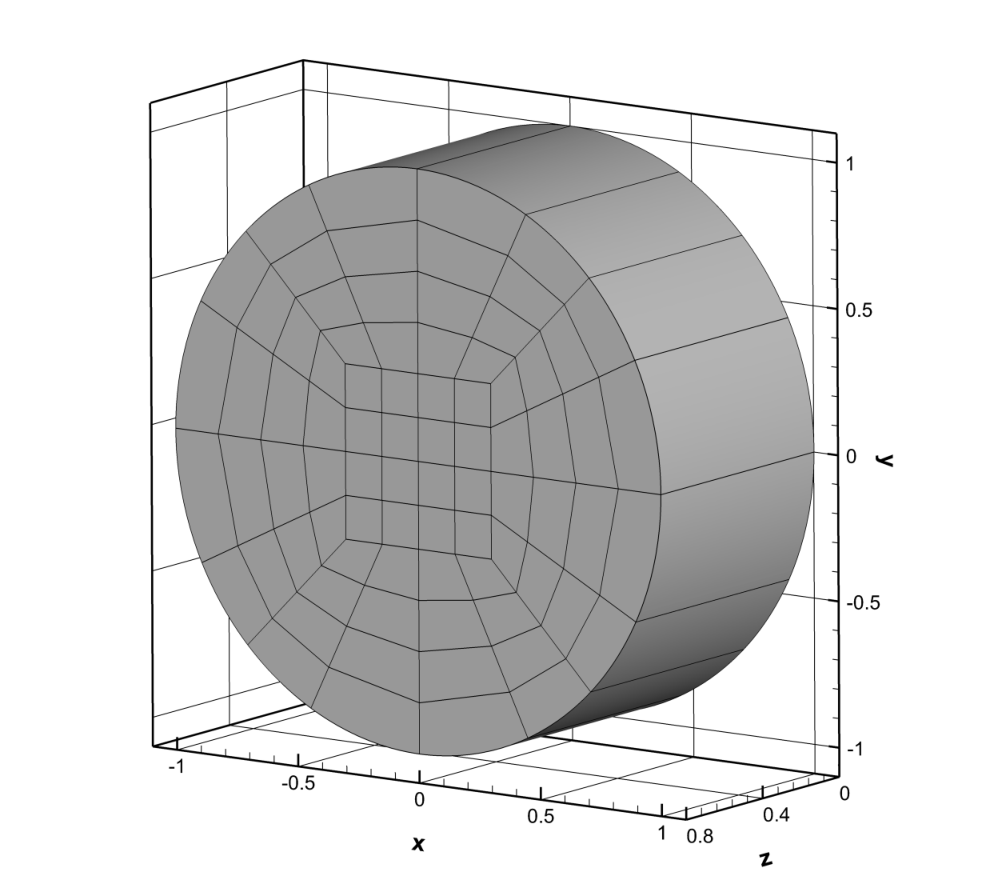
In this subsection we simulate the co-current flow of two immiscible incompressible fluids in a circular pipe, and compare simulation results with the theoretical solution to this problem to test the accuracy of the method developed herein.

Consider a fully-developed laminar co-current flow of two immiscible incompressible Newtonian fluids in a circular pipe. The radius of the pipe is $r_{2}$ . We assume that there is no interface instability between the two fluids and that the surface tension between them is zero. The first fluid occupies the inner core region $0\leqslant r\leqslant r_{1}$ , where $0<r_{1}<r_{2}$ , and the second fluid occupies the outer region $r1\leqslant r\leqslant r_{2}$ . The flow is driven by a pressure gradient $\bar{K}$ along the axial direction. Note that the flow is fully developed. There is no radial or azimuthal flow, and the only non-zero velocity component is in the axial direction. We assume zero gravity in this problem. Let $\mu_{1}$ and $\mu_{2}$ denote the dynamic viscosities of the two fluids. Note that the densities of the fluids have no effect on the fully-developed velocity profiles, and so they are both taken as unit values in the simulation.

This problem has an exact physical solution. The axial velocity profiles for the two fluids are given by [25]:

	$\frac{w_{1}(r)}{\bar{w}}=\frac{2\left(1-\frac{r_{1}^{2}}{r_{2}^{2}}+\frac{\mu_{2}}{\mu_{1}}\frac{r_{1}^{2}-r^{2}}{r_{2}^{2}}\right)}{\frac{r_{1}^{4}}{r_{2}^{4}}\left(\frac{\mu_{2}}{\mu_{1}}-1\right)+1},\quad 0\leqslant r\leqslant r_{1},$		(51a)
	$\frac{w_{2}(r)}{\bar{w}}=\frac{2\left[1-\left(\frac{r}{r_{2}}\right)^{2}\right]}{\frac{r_{1}^{4}}{r_{2}^{4}}\left(\frac{\mu_{2}}{\mu_{1}}-1\right)+1},\quad r_{1}\leqslant r\leqslant r_{2},$		(51b)

where $w_{1}$ and $w_{2}$ denote the axial velocities of the first and second fluids respectively. $\bar{w}$ is the average velocity across the pipe, given by

\bar{w}=\frac{\bar{K}r_{2}^{2}}{8\mu_{2}}\left[\frac{r_{1}^{4}}{r_{2}^{4}}\left(\frac{\mu_{2}}{\mu_{1}}-1\right)+1\right].

(52)

We will simulate this problem and compare the results with the analytic expressions given by equations (51a)–(51b).

We consider a computational domain shown in Figure 2. The axial dimension of the domain is $\frac{4}{5}r_{2}$ . All flow variables are assumed to be periodic along the axial direction. When the surface tension is zero ( $\sigma=0$ ), $\lambda=\frac{3}{2\sqrt{2}}\sigma\eta=0$ , and the very nature of the partial differential equation (3c) for the phase field function changes, because of disappearance of the terms containing the highest derivatives on the right hand side. Our current implementation of the algorithm cannot handle this case for the convection equation. But we note that with the convection equation, the phase field function is convected along the pipe with the axial velocity, and its equilibrium distribution will have isofaces that are cylindrical surfaces around the pipe axis. So for this problem we will employ the following distribution for the phase field function, $\phi(\mathbf{x})=-\tanh\frac{\sqrt{x^{2}+y^{2}}-r_{1}}{\sqrt{2}\eta}$ ( $\eta$ is the interfacial thickness scale) for solving the momentum equations (3a)–(3b). The equation (3c) with $\lambda=0$ , which reduces to the convection equation, will not be solved. No-slip condition for the velocity is imposed on the pipe wall.

We use the pipe radius $r_{2}$ as the length scale $L$ , and the fluid density (same density for the two fluids) as the density scale $\varrho_{d}$ . The velocity scale is chosen as $U_{0}=10\sqrt{|\bar{K}|L}$ , where $\bar{K}$ is the pressure drop along the pipe axis over a unit length. All the flow variables and parameters are then normalized based on the constants given in Table 1.

(a) (b)

Figure 3: Steady-state axial velocity profiles obtained using different interfacial thickness scale

\eta

(a), and different element orders (b). In (a) a fixed element order

10

is employed, and in (b) a fixed

\eta=0.0005

is employed.

We discretize the computational domain using $16$ Fourier planes along the axial ( $z$ ) direction. Each plane is discretized using a mesh of $80$ quadrilateral spectral elements (see Figure 2), and the element order is varied over a range of values in the tests. Values for the non-dimensionalized simulation parameters are given below:

\begin{cases}r_{1}=0.5,\;r_{2}=1,\ \mu_{1}=0.01,\ \frac{\mu_{2}}{\mu_{1}}=6,\ \rho_{1}=\rho_{2}=1,\\ \bar{K}=-0.01,\ \eta=0.0005\ \text{(or varied)},\;J=2,\;\text{element order}=10\sim 14,\\ \Delta t=5\times 10^{-5}.\end{cases}

(53)

Starting with an initial zero velocity field, we have performed a long-time simulation of this problem using the method from Section 2, until the flow has reached a steady state. Figure 3(a) shows a study of the effect of the interfacial thickness scale $\eta$ in the phase field distribution on the simulation results. Here we plot the steady-state axial velocity profiles obtained with several $\eta$ values ranging between $0.01$ and $0.0005$ . A fixed element order $10$ is employed in these simulations. In the region of the outer fluid, the velocity profiles obtained with the various $\eta$ values overlap with one another. In the region of the inner fluid, on the other hand, some differences can be observed. As $\eta$ decreases from $0.01$ , we initially observe an increase in the velocity magnitude in the inner fluid region. When $\eta$ is decreased further (below about $\eta=0.001$ ), no significant change in the velocity profiles can be observed.

Figure 4: Comparison of steady-state axial velocity profiles from current simulation and the exact physical solution of [25]

Fig. 3(b) illustrates the effect of the spatial resolution in the simulations. It is a plot of the profiles of the steady-state axial velocity across the pipe obtained using several element orders ranging from $10$ to $14$ in the simulations. The interfacial thickness scale is fixed at $\eta=0.0005$ in these simulations. The velocity profiles obtained with different element orders essentially overlap with one another, with a negligible difference. This suggests that these element orders and the spatial resolutions are adequate for the simulations of the current problem.

Fig. 4 compares the steady-state axial velocity profiles obtained from the current simulation and the exact physical solution given by [25]. The simulation result corresponds to an element order $14$ and the interfacial thickness scale $\eta=0.0005$ . We observe that the simulation result is in good agreement with the theoretical result, suggesting that our method has captured the flow field accurately.

3.3 Equilibrium Shape of a Liquid Drop on a Partially Wettable Wall

In this subsection, we study the equilibrium configuration of a liquid drop on a horizontal wall that is partially wettable. The effect of the contact angle on the equilibrium drop shape will be investigated under zero gravity.

More specifically, we consider a liquid drop (the second fluid) in an ambient lighter liquid (the first fluid); see Figure 5 for a sketch of the problem. The liquid drop (hemisphere) and the ambient fluid are initially at rest on a horizontal wall with certain wetting properties. The gravity is assumed to be zero for this problem. The system is then released, and the drop starts to evolve under the effect of surface tension between the two fluids and the imposed contact angle at the wall, eventually reaching an equilibrium state. According to [6], the liquid drop becomes a spherical cap at equilibrium. We can define the spreading length (diameter of the drop base) and the drop height for the equilibrium shape; see Figure 5 for a sketch of these parameters. Our goal here is to study the equilibrium configuration of the drop, and compare the simulation results with the theoretical results from [6].

To simulate the problem, we consider the flow domain given by $\Omega=\left\{(x,y,z):-\frac{L}{2}\leqslant x\leqslant\frac{L}{2},0\leqslant y\leqslant\frac{L}{2},0\leqslant z\leqslant\frac{4L}{5}\right\}$ as sketched in Figure 5, where $L$ is a characteristic length scale. The initial drop shape is assumed to be a hemisphere with radius $R_{0}=\frac{L}{4}$ . We choose the density of the first fluid as the characteristic density scale, i.e. $\varrho_{d}=\rho_{1}$ . We choose the characteristic velocity scale as $U_{0}=\frac{1}{10}\sqrt{\frac{\sigma}{\varrho_{d}L}}$ , where $\sigma$ is the surface tension. All the physical variables and parameters are then normalized based on Table 1.

Let R denote the radius of the spherical cap at equilibrium and $\theta_{e}$ denote the contact angle measured on the side of the heavier fluid (i.e. the second fluid). Then, based on the conservation of the volume of the liquid drop, one can obtain the theoretical values of the spreading length and the drop height at equilibrium as follows [6]:

\frac{R}{R_{0}}=\sqrt[3]{\frac{2}{(2+\cos\theta_{e})(1-\cos\theta_{e})^{2}}},\;L_{s}=2R\sin\theta_{e},\;H=R(1-\cos\theta_{e})

(54)

where $R_{0}$ is the radius of the initial hemisphere, $L_{s}$ is the spreading length, and $H$ is the drop height.

Along the $x$ and $z$ directions we impose periodic conditions for all the flow variables. The top and bottom boundaries (i.e. $y=0$ and $y=\frac{L}{2}$ ) are assumed to be solid walls, and we impose the no-slip condition for the velocity and the contact-angle boundary conditions (with $g_{a}=0$ and $g_{c}=0$ ) for the phase field function. To simulate the problem we discretize the flow domain using $96$ Fourier planes along the z direction, and each plane is further discretized using a mesh of $200$ quadrilateral spectral elements (with $20$ elements along the $x$ direction and $10$ elements along the $y$ direction). The source term in the Cahn-Hilliard equation is set to $g=0$ . A number of contact angles ranging from $\theta_{e}=60^{0}$ to $120^{0}$ are considered in the simulations. The following non-dimensional parameter values have been used in the simulations:

\begin{cases}\rho_{1}=1,\;\frac{\rho_{2}}{\rho_{1}}=5,\;\mu_{1}=0.05,\ \frac{\mu_{2}}{\mu_{1}}=2,\ \text{element order}=8\sim 12,\\ \eta=0.01,\ \sigma=100,\ \lambda=\frac{3}{2\sqrt{2}}\sigma\eta,\ \gamma_{1}=\frac{10^{-8}}{\lambda}\\ \rho_{0}=\min(\rho_{1},\rho_{2}),\ \nu_{m}=\frac{\max(\mu_{1},\mu_{2})}{\min(\rho_{1},\rho_{2})},\ \Delta t=1\times 10^{-5},\ J=2.\end{cases}

Figures 6(a) and 6(b) show the equilibrium shapes of the liquid drop corresponding to the contact angles $\theta_{e}=60^{0}$ and $\theta_{e}=120^{0}$ respectively. Plotted here is the iso-surface $\phi=0$ for the phase field function. It is evident that the drop resembles a spherical cap at equilibrium, qualitatively consistent with the theory [6].

To make a quantitative comparison between the simulation and theory, we need to extract and compute several parameters from the simulation data. Figure 7 illustrates how to extract the spreading length and the height of the equilibrium drop. It shows a projection of the iso-surface $\phi=0$ onto the $x-y$ plane using the visualization software Tecplot 360, which corresponds to a contact angle $\theta_{e}=105^{0}$ . From the figure we can determine the minimum and the maximum coordinates of the drop base along the $x$ direction, denoted by $X_{\min}$ and $X_{\max}$ respectively. Then the spreading length is $L_{s}=X_{\max}-X_{\min}$ . Similarly, the minimum and the maximum coordinates of the drop profile in the $y$ direction can also be determined, denoted by $Y_{\min}$ ( $Y_{\min}=0$ ) and $Y_{\max}$ respectively. The drop height is given by $H=Y_{\max}-Y_{\min}$ . According to equation (54),

\frac{L_{s}}{H}=\frac{2\sin\theta_{e}}{1-\cos\theta_{e}}.

(55)

Therefore, once the spreading length $L_{s}$ and the drop height $H$ are calculated, we can solve equation (55) to obtain the actual contact angle based on the simulated drop profile, which can then be compared with the angle imposed through the contact-angle boundary condition.

Table 2: Effect of spatial resolution (element order) on the spreading length (

L_{s}/R_{0}

) and the drop height (

H/R_{0}

). The contact angle is

\theta_{e}=105^{0}

	Element Order	Spreading Length	Drop Height
Simulation	8	0.432	0.283
	10	0.433	0.282
	12	0.433	0.282
Theoretical		0.434	0.283

Table 2 shows results of the resolution test for this problem. We list the spreading length and the drop height obtained from the simulations using three element orders ( $8$ , $10$ and $12$ ) corresponding to an imposed contact angle $\theta_{e}=105^{0}$ . The theoretical values of these parameters, computed based on equation (54), are also included for comparison. We observe that the change in these parameters values are negligible with the increase of the element order, indicating the adequacy of the mesh resolutions for the current problem. We can also observe that the values from the simulations agree well with those of the theoretical values. Based on the resolution test, we have employed an element order $10$ in the majority of simulations.

Figure 8: Comparison of the drop height and spreading length (normalized by

R_{0}

) as a function of the imposed contact angle between the simulation and the theory. Comparison of the actual contact angle obtained from the simulated drop profiles with the imposed contact angle is also shown. The left vertical axis is for the drop height and spreading length, and the right axis is for the contact angle (in degrees).

We have varied the imposed contact angle systematically between $60^{0}$ and $120^{0}$ , and computed the spreading length, the drop height, and the actual contact angle obtained from the simulated drop profiles at equilibrium. Figure 8 shows a comparison of these quantities as a function of the imposed contact angle between the simulation and the theoretical results. The theoretical values for the spreading length and the drop height are computed based on equation (54). The actual contact angles obtained from the drop profiles are computed based on equation (55). It is observed that the simulation results agree well with the theoretical values. These results indicate that our method has captured these flow parameters accurately.

3.4 Dynamics of a Rising Air Bubble in Water

In this subsection, we use the method developed herein to study the rise of an air bubble through water in a wall-bounded domain. The goal is to investigate the effect of the contact angle on the dynamics of the fluid interfaces, and to demonstrate the potential of the method for two-phase problems under realistic physical parameters such as the density ratios and viscosity ratios.

Specifically, we consider a three-dimensional domain with dimensions $1cm\times 1.4cm\times 1.4cm$ along the three directions; see Figure 9(a) for illustration. The top and the bottom sides of the domain are solid walls, while in the $x$ and $z$ directions the domain is periodic. The domain is filled with water. An air bubble, initially spherical with a radius $2.5mm$ , is trapped in the water (at rest), with its center located $5mm$ above the bottom wall. The gravity is assumed to point downward ( $-y$ direction). At $t=0$ , the system is released. The air bubble rises through the water due to buoyancy, and touches the upper boundary to form an air dome attached to the upper wall. We will employ the method developed in Section 2 to investigate this dynamic process and the topological changes of the air bubble. The physical parameter values of the air and water employed in the current problem are listed in Table 3.

	Air	Water
Density [ $kg/m^{3}$ ]	$1.204$	$998.207$
Dynamic viscosity [ $kg/(m\cdot s)$ ]	$1.78\times 10^{-5}$	$1.002\times 10^{-3}$
Surface tension [ $kg/s^{2}$ ]	$0.0728$
Gravitational acceleration [ $m/s^{2}$ ]	$9.8$

Table 3: Physical properties for the air and water.

We set up a coordinate system, in which the domain is given by $-\frac{L}{2}\leqslant x\leqslant\frac{L}{2}$ , $0\leqslant y\leqslant\frac{7L}{5}$ , and $0\leqslant z\leqslant\frac{7L}{5}L$ , where $L=1cm$ is the characteristic length scale. We use the air density as the characteristic density scale, $\varrho_{d}=1.204kg/m^{3}$ . We choose the characteristic velocity scale as $U_{0}=\sqrt{g_{0}L}$ , where $g_{0}=1m/s^{2}$ . The normalization of the physical variables and parameters is then performed according to Table 1.

In the simulations the air and the water are chosen as the first and the second fluids, respectively. The flow domain is discretized using $96$ Fourier planes along the $z$ direction, and each $x$ - $y$ plane is discretized with a mesh of $200$ quadrilateral elements (with an element order $12$ ). Periodic boundary conditions are imposed for all flow variables along the $x$ direction (at $x=\pm\frac{L}{2}$ ). Periodic conditions are also enforced in the $z$ direction because of the Fourier spectral expansion in this direction. On the top and bottom walls, a no-slip condition (zero velocity) is imposed for the velocity, and the contact-angle conditions (5b)–(5c) with $g_{c}=0$ and $g_{b}=0$ are imposed for the phase field function. The initial velocity is set to zero, and the initial distribution of the phase field function is given by

\phi_{in}(\textbf{x})=-\tanh\frac{\sqrt{(x-x_{0})^{2}+(y-y_{0})^{2}+(z-z_{0})^{2}}-R_{0}}{\sqrt{2}\eta},

(56)

where $R_{0}=\frac{L}{4}$ is the initial radius of the air bubble, and $(x_{0},y_{0},z_{0})=(0,0.5L,0.7L)$ is the initial coordinate of the center of bubble. A number of contact angles ranging from $60^{0}$ to $105^{0}$ have been considered in the simulations, which correspond to hydrophilic and hydrophobic walls. Here the contact angle refers to the angle formed between the air/water interface and the wall measured on the side of the water. The values of the non-dimensionalized simulation parameters for this problem are given below:

\begin{cases}\rho_{1}=1,\;\frac{\rho_{2}}{\rho_{1}}=829,\;\mu_{1}=0.0147828,\;\frac{\mu_{2}}{\mu_{1}}=56.29,\\ \sigma=604.601,\ \eta=0.02,\ \lambda=\frac{3}{2\sqrt{2}}\sigma\eta,\ \gamma_{1}=\frac{10^{-6}}{\lambda},\\ \rho_{0}=\min(\rho_{1},\rho_{2}),\ \nu_{m}=\max\left(\frac{\mu_{1}}{\rho_{1}},\frac{\mu_{2}}{\rho_{2}}\right),\\ 96\ \text{planes in z},\ 200\ \text{elements per plane},\ \text{element order}=12,\;\Delta t=2.5\times 10^{-5}.\\ \text{contact angle:}\ 60^{0}\sim 105^{0}\end{cases}

We have conducted simulations of this air/water two-phase problem under several contact angles, and let us now look into the dynamics of the system. Figure 9 shows a temporal sequence of snapshots of the air/water interface in the flow, which correspond to a contact angle $60^{0}$ (hydrophilic wall). The fluid interface is visualized by the iso-surface $\phi=0$ of the phase field function. It is observed that as the system is released the air bubble rises through the water due to buoyancy, and that the bubble experiences a notable deformation (Figures 9(a)-(c)). Then as the bubble touches the upper wall, a topological change in the air-water interface occurs (Figures 9(d)-(e)). We observe that the air-water interface, which was originally a single piece separating the bulk of air and water, splits into two pieces (Figures 9(e)-(f)) on the upper wall. The inner piece of interface traps a small pocket of water on the wall. It evolves into a small water drop that is suspended from the upper wall and trapped inside the bulk of air (Figures 9(f)-(h)). The outer piece of interface separates the air from the bulk of water, and it evolves into a spherical cap attached to the upper wall over time (Figure 9(h)).

Figure 10 illustrates the dynamics of the air bubble corresponding to a contact angle of $90^{0}$ (neutral wettability). We observe a behavior similar to that with the contact angle of $60^{0}$ at the early stage, before the bubble reaches the wall. But when the bubble touches the upper wall, the system exhibits some notable difference in the dynamics, and in this case it is notably more complicated. With the $90^{0}$ contact angle, after the air/water interface breaks up into two individual pieces, the pocket of water trapped by the inner piece of interface appears more mobile on the upper wall (Figures 10(e)-(i)). As the surface area of the water pocket contracts due to surface tension, the contact line formed between this interface and the wall moves inward and the base of the water pocket shrinks on the wall (Figures 10(e)-(g)). As a result, the water deforms into a long slender column at some point (Figure 10(h)). Simultaneously, the contact line formed between the outer piece of the air/water interface and the wall moves outward, as the bulk of air spreads outward on the upper wall (Figures 10(f)-(h)). The pillar-like inner interface and the dome-like outer interface touches each other and re-connects near the center, and a certain amount of water escapes from the drop on the upper wall into the bulk of water (Figures 10(h)-(i)). Afterward, the two pieces of interface pinches off and separates again. The inner interface shrinks and traps the residual water to form a smaller drop on the upper wall (Figures 10(k)-(l)), while the outer interface evolves into a hemisphere eventually (Figure 10(l)).

Figure 11 shows the motion of the air bubble with a contact angle $105^{0}$ , which corresponds to a hydrophobic wall. The same dynamic behavior can be observed of the bubble at the initial stage, before it touches the upper wall (Figures 11(a)-(c)). Compared with the other cases, the configuration of the system is significantly different after the bubble breaks up on the upper wall. At this contact angle, as the base of the water drop trapped by the inner interface shrinks on the upper wall due to the contact line motion, the surface tension apparently can no longer sustain the weight of the water on the wall. We observe that the small water drop completely detaches from the wall. It drips onto the outer piece of interface, and merges into the bulk of water (Figures 11(f)-(j)). The deformation caused to the outer air/water interface due to this process is clearly visible from Figures 11(g) and 11(i)-(j). Only the air dome (without the small water drop inside) is left on the upper wall for this case (Figure 11(l)).

With the $60^{0}$ contact angle, the pocket of water trapped by the inner interface becomes a water drop suspended on the upper wall. As the contact angle increases, the trapped water drop can become unstable and some water may escape from the wall due to the interactions among the inertia (contact line motion), contact angle, gravity and the surface tension. For the $90^{0}$ contact angle, a portion of the trapped water escapes from the air bubble, and some remains at the wall. This seems to be because the surface tension is not strong enough to carry the massive water drop and overcome the inertia due to the contact line motion. But once some of the water escapes, it is sufficient to stabilize the lighter drop. For the air-water interface with the $105^{0}$ contact angle, the trapped water drop completely escapes from the air-bubble into the bulk of water, and there is once more only a single air-water interface. The trapped water overall tends to break free from the wall more likely with a larger contact angle.

The results of this section show that the method developed herein can effectively capture the three-dimensional two-phase flow dynamics under large and realistic density ratios and viscosity ratios. The method will be useful for studying the interactions between fluid interfaces and solid walls, large interfacial deformations and topological changes of the interfaces.

4 Concluding Remarks

The current work is focused on three-dimensional two-phase flows on domains with at least one homogeneous direction. We have presented a hybrid spectral element-Fourier spectral method for efficient simulations of this class of 3D two-phase problems. A critical component of this method is a strategy we developed in a previous work for dealing with the variable density/viscosity of the two-phase mixture, which makes the efficient use of FFTs in the current work possible for these flows with different densities and viscosities for the two fluids. Our method transforms the computation of two-phase flows in the 3D space into a set of computations in the 2D planes of the non-homogeneous directions, which are completely de-coupled from one another. Therefore, only a series of 2D problems need to be solved, which can be performed in parallel.

Extensive numerical tests with several wall-bounded two-phase flows in 3D space have been presented to assess the accuracy and performance of the method. Comparisons with theoretical results demonstrate that the presented method can capture the physical effects such as those of the surface tension and the contact angles accurately in 3D. Simulation results show that our method can effectively deal with the topological changes of the fluid interface, the moving contact lines, and the interaction between fluid interfaces and solid walls in the 3D space.

The presented method can be an efficient technique for investigating a wide class of two-phase problems such as the oil transport in the pipe, wind/ocean-wave interactions, and the dynamics of contact lines. We anticipate that it will be useful and instrumental in a number of areas such as microfluidics, surface ship hydrodynamics, and the study of functional surfaces.

Acknowledgment

The work of S.H.C. and S.D. was partially supported by the NSF DMS-1318820 and DMS-1522537. L.D.Z. acknowledges the support of NSF DMS-1522554.

References

[1] H. Abels, H. Garcke, and G. Grün. Thermodynamically consistent, frame indifferent diffuse interface models for incompressible two-phase flows with different densities. Mathematical Models and Methods in Applied Sciences, 22:1150013, 2012.
[2] Sebastian Aland and Feng Chen. An efficient and energy stable scheme for a phase-field model for the moving contact line problem. International Journal for Numerical Methods in Fluids, 81(11):657–671, August 2016.
[3] D. M. Anderson, G. B. McFadden, and A. A. Wheeler. Diffuse-interface methods in fluid mechanics. Annual Review of Fluid Mechanics, 30(1):139–165, 1998.
[4] V.E. Badalassi, H.D. Ceniceros, and S. Banerjee. Computation of multiphase systems with phase field models. J. Comput. Phys., 190:371–397, 2003.
[5] A. Carlson, M. Do-Quang, and G. Amberg. Dissipation in rapid dynamic wetting. J. Fluid Mech., 682, 2011.
[6] P.G. de Gennes, F. Brochard-Wyart, and D. Quere. Capillarity and Wetting Phenomena. Springer, 2003.
[7] H. Ding, P.D.M. Spelt, and C. Shu. Diffuse interface model for incompressible two-phase flows with large density ratios. J. Comput. Phys., 226:2078–2095, 2007.
[8] S. Dong. Direct numerical simulation of turbulent Taylor-Couette flow. J. Fluid Mech., 587:373–393, 2007.
[9] S. Dong. On imposing dynamic contact-angle boundary conditions for wall-bounded liquid-gas flows. Computer Methods in Applied Mechanics and Engineering, 247–248:179–200, 2012.
[10] S. Dong. An efficient algorithm for incompressible N-phase flows. Journal of Computational Physics, 276:691–728, 2014.
[11] S. Dong. An outflow boundary condition and algorithm for incompressible two-phase flows with phase field approach. Journal of Computational Physics, 266:47–73, 2014.
[12] S. Dong. Wall-bounded multiphase flows of $N$ immiscible incompressible fluids: consistency and contact-angle boundary condition. Journal of Computational Physics, 338:21–67, 2017.
[13] S. Dong. Multiphase flows of N immiscible incompressible fluids: A reduction-consistent and thermodynamically-consistent formulation and associated algorithm. Journal of Computational Physics, 361:1–49, 2018.
[14] S. Dong, G.E. Karniadakis, A. Ekmekci, and D. Rockwell. A combined DNS-PIV study of the turbulent near wake. J. Fluid Mech., 569:185–207, 2006.
[15] S. Dong and J. Shen. A time-stepping scheme involving constant coefficient matrices for phase field simulations of two-phase incompressible flows with large density ratios. Journal of Computational Physics, 231:5788–5804, 2012.
[16] S. Dong and X. Zheng. Direct numerical simulation of spiral turbulence. J. Fluid Mech., 668:150–173, 2011.
[17] Yuezheng Gong, Jia Zhao, and Qi Wang. Second order fully discrete energy stable methods on staggered grids for hydrodynamic phase field models of binary viscous fluids. SIAM Journal on Scientific Computing, 40(2):528–553, 2018.
[18] D. Jacqmin. Calculation of two-phase navier-stokes flows using phase-field modeling. J. Comput. Phys., 155:96–127, 1999.
[19] D. Jacqmin. Contact-line dynamics of a diffuse fluid interface. J. Fluid Mech., 402:57–88, 2000.
[20] G.E. Karniadakis and S.J. Sherwin. Spectral/hp element methods for computational fluid dynamics, 2nd edition. Oxford University Press, 2005.
[21] J. Kim. Phase field models for multi-component fluid flows. Comm. Comput. Phys., 12:613–661, 2012.
[22] C. Liu and J. Shen. A phase field model for the mixture of two incompressible fluids and its approximation by a Fourier-spectral method. Physica D, 179:211–228, 2003.
[23] J. Lowengrub and L. Truskinovsky. Quasi-incompressible Cahn-Hilliard fluids and topological transitions. Proceedings of the Royal Society A, 454:2617–2654, 1998.
[24] X. Ma, G.-S. Karamanos, and G.E. Karniadakis. Dynamics and low-dimensionality of a turbulent near wake. Journal of Fluid Mechanics, 410:29–65, 2000.
[25] E. Nogueira and R. Cotta. Heat transfer solutions in laminar co-current flow of immiscible liquids. Wärme - und Stoffübertragung, 25(6):361–367, November 1990.
[26] S.J. Osher and J.A. Sethian. Fronts propagating with curvature dependent speed: algorithms based on hamilton-jacobi formulations. J. Comput. Phys., 79:12–49, 1988.
[27] T. Qian, X.-P. Wang, and P. Sheng. A variational approach to moving contact line hydrodynamics. J. Fluid Mech., 564:333–360, 2006.
[28] R. Scardovelli and S. Zaleski. Direct numerical simulation of free-surface and interfacial flow. Annu. Rev. Fluid Mech., 31:567–603, 1999.
[29] J. A. Sethian and Peter Smereka. Level set methods for fluid interfaces. Annual Review of Fluid Mechanics, 35(1):341–372, January 2003.
[30] J. Shen and X. Yang. A phase-field model and its numerical approximation for two-phase incompressible flows with different densities and viscosities. SIAM J. Sci. Comput., 32:1159–1179, 2010.
[31] J. Shen, X. Yang, and H. Yu. Efficient energy stable numerical schemes for a phase field moving contact line model. Journal of Computational Physics, 284:617–630, 2015.
[32] S.J. Sherwin and G.E. Karniadakis. A triangular spectral element method: applications to the incompressible Navier-Stokes equations. Computer Methods in Applied Mechanics and Engineering, 123:189–229, 1995.
[33] G. Tryggvason, B. Bunner, A. Esmaeeli, D. Juric, N. Al-Rawahi, W. Tauber, J. Han, S. Nas, and Y.-J. Jan. A front-tracking method for the computations of multiphase flow. Journal of Computational Physics, 169(2):708–759, May 2001.
[34] C.H.K. Williamson. Vortex dynamics in a cylinder wake. Annual Review of Fluid Dynamics, 28:477–539, 1996.
[35] P. Yue, J.J. Feng, C. Liu, and J. Shen. A diffuse-interface method for simulating two-phase flows of complex fluids. Journal of Fluid Mechanics, 515:293–317, 2004.
[36] P. Yue, C. Zhou, and J.J. Feng. Sharp-interface limit of the Cahn-Hilliard model for moving contact lines. J. Fluid Mech., 645:279–294, 2010.
[37] X. Zheng and S. Dong. An eigen-based high-order expansion basis for structured spectral elements. Journal of Computational Physics, 230:8573–8602, 2011.