Long-range interactions of kinks

Consider a real scalar field $\varphi(x,t)$ in $(1+1)$ dimensional space-time, with its dynamics determined by the Lagrangian density

$$\mathscr{L}=\frac{1}{2}\left(\frac{\partial\varphi}{\partial t}\right)^{2}-\frac{1}{2}\left(\frac{\partial\varphi}{\partial x}\right)^{2}-V(\varphi),$$

(1)

where $V(\varphi)$ is a potential that defines the self-interaction of the field $\varphi$. The energy functional corresponding to the Lagrangian (1) is

$$E[\varphi]=\int_{-\infty}^{+\infty}\left[\frac{1}{2}\left(\frac{\partial\varphi}{\partial t}\right)^{2}+\frac{1}{2}\left(\frac{\partial\varphi}{\partial x}\right)^{2}+V(\varphi)\right]dx.$$

(2)

Assume that the potential $V(\varphi)$ is a non-negative polynomial of even degree (denoted in short-hand as “$\varphi^{2n}$”) having two or more minima $\bar{\varphi}_{1}$, $\bar{\varphi}_{2}$, $\ldots$, $\bar{\varphi}_{n}$ of equal depth $V(\bar{\varphi}_{1})=V(\bar{\varphi}_{2})=\cdots=V(\bar{\varphi}_{n})=0$. Consider two adjacent minima $\bar{\varphi}_{i}$ and $\bar{\varphi}_{i+1}$. Let $\varphi_{\mathrm{K}}(x)$ be a kink (see, e.g. (manton, Ch. 5)) interpolating between these minima, i.e.,

$$\lim\limits_{x\to-\infty}\varphi_{\mathrm{K}}(x)=\bar{\varphi}_{i},\qquad\lim\limits_{x\to+\infty}\varphi_{\mathrm{K}}(x)=\bar{\varphi}_{i+1}.$$

(3)

According to conventional notation, we can say that this kink belongs to the topological sector $(\bar{\varphi}_{i},\bar{\varphi}_{i+1})$, and we denote it by $\varphi_{(\bar{\varphi}_{i},\bar{\varphi}_{i+1})}(x)$.

The Euler–Lagrange equation of motion, which is the condition for extremizing the action generated by the Lagrangian density (1), is

$$\frac{\partial^{2}\varphi}{\partial t^{2}}=\frac{\partial^{2}\varphi}{\partial x^{2}}-V^{\prime}(\varphi).$$

(4)

The kink shape function $\varphi=\varphi_{\mathrm{K}}(x)$ is a time-independent solution of Eq. (4), and it can be shown that it satisfies a first-order ordinary differential equation:

$$\frac{d\varphi}{dx}=\sqrt{2V(\varphi)}.$$

(5)

A static field configuration that satisfies Eq. (5) has the minimal energy among all the configurations in a given topological sector. The solutions that satisfy Eq. (5) are called BPS-saturated configurations (BPS standing for Bogomolny–Prasad–Sommerfield) bps. Moving kinks can be obtained from solutions of Eq. (5) via a boost transformation owing to the Lorentz invariance of the field theory. Using Eq. (5), the energy (2) can be rewritten as

$$E[\varphi]=\int_{-\infty}^{+\infty}\sqrt{2V(\varphi)}\cdot\sqrt{2V(\varphi)}\>dx.$$

(6)

Taking into account that $\sqrt{2V(\varphi)}\>dx=d\varphi$, the energy (rest mass) of a static BPS-saturated field configuration is

$$M=\int_{\bar{\varphi}_{i}}^{\bar{\varphi}_{i+1}}\sqrt{2V(\varphi)}\>d\varphi.$$

(7)

Now, we formulate general conditions that must be satisfied in order for the model to have kinks with power-law tail asymptotics. We also give general formulæ for such asymptotics. Let us turn our attention to the potential $V(\varphi)$. Let $\bar{\varphi}_{i}$ and $\bar{\varphi}_{i+1}$ be zeros of the function $V(\varphi)$ of orders $k_{i}$ and $k_{i+1}$, respectively. Notice that $k_{i}$ and $k_{i+1}$ must be even. We assume $\bar{\varphi}_{i}<\bar{\varphi}_{i+1}$, for definiteness. Then, the potential $V(\varphi)$ can be written as

$$V(\varphi)=\left(\varphi-\bar{\varphi}_{i}\right)^{k_{i}}\left(\varphi-\bar{\varphi}_{i+1}\right)^{k_{i+1}}V_{1}(\varphi),$$

(8)

where $V_{1}(\bar{\varphi}_{i})>0$, $V_{1}(\bar{\varphi}_{i+1})>0$. Inserting Eq. (8) into Eq. (5) and recalling that $\bar{\varphi}_{i}<\varphi<\bar{\varphi}_{i+1}$, we obtain after integrating:

$$\int dx=\int\frac{d\varphi}{\left(\varphi-\bar{\varphi}_{i}\right)^{k_{i}/2}\left(\bar{\varphi}_{i+1}-\varphi\right)^{k_{i+1}/2}\sqrt{2V_{1}(\varphi)}}\,.$$

(9)

To find asymptotics of the kink $\varphi_{(\bar{\varphi}_{i},\bar{\varphi}_{i+1})}(x)$ as $x\to-\infty$, we use the fact that $\varphi\to\bar{\varphi}_{i}$ in this limit. Then, there are slowly varying factors within the integrand in the right-hand side of Eq. (9) at $\varphi\to\bar{\varphi}_{i}$. These factors can be (approximately) taken out from the integral. As a result, we obtain an asymptotic equality:

$$\int dx\approx\frac{1}{\left(\bar{\varphi}_{i+1}-\bar{\varphi}_{i}\right)^{k_{i+1}/2}\sqrt{2V_{1}(\bar{\varphi}_{i})}}\int\frac{d\varphi}{\left(\varphi-\bar{\varphi}_{i}\right)^{k_{i}/2}}\,.$$

(10)

Integration of the right-hand side gives power-law dependence, if $k_{i}>2$. Taking this observation into account, we obtain the asymptotics of the kink as $x\to-\infty$:

$$\varphi_{(\bar{\varphi}_{i},\bar{\varphi}_{i+1})}(x)\approx\bar{\varphi}_{i}+\left[\frac{2}{(k_{i}-2)\left(\bar{\varphi}_{i+1}-\bar{\varphi}_{i}\right)^{k_{i+1}/2}\sqrt{2V_{1}(\bar{\varphi}_{i})}}\right]^{2/(k_{i}-2)}\frac{1}{|x|^{2/(k_{i}-2)}}\,.$$

(11)

Similarly, for case of $k_{i+1}>2$, we obtain asymptotics of the kink as $x\to+\infty$:

$$\varphi_{(\bar{\varphi}_{i},\bar{\varphi}_{i+1})}(x)\approx\bar{\varphi}_{i+1}-\left[\frac{2}{(k_{i+1}-2)\left(\bar{\varphi}_{i+1}-\bar{\varphi}_{i}\right)^{k_{i}/2}\sqrt{2V_{1}(\bar{\varphi}_{i+1})}}\right]^{2/(k_{i+1}-2)}\frac{1}{x^{2/(k_{i+1}-2)}}\,.$$

(12)

Below, we will use Eqs. (11) and (12) to find power-law asymptotics of kinks of a $\varphi^{8}$ model. Note that exponential asymptotics could be found by integrating Eq. (10) for the case of $k_{i}=2$, but a further refinement of our approximations is needed to capture the prefactor of the exponential.

As our featured example, we consider the triple-well $\varphi^{8}$ potential

$$V(\varphi)=\varphi^{4}(1-\varphi^{2})^{2}.$$

(13)

This potential has three minima: $\bar{\varphi}_{1}=-1$, $\bar{\varphi}_{2}=0$, and $\bar{\varphi}_{3}=1$. Hence, there are two kinks in the model, $\varphi_{(-1,0)}(x)$ and $\varphi_{(0,1)}(x)$, and two corresponding antikinks.

Inserting the potential (13) into Eq. (5) and requiring that $0<|\varphi|<1$, we have

$$\frac{d\varphi}{\varphi^{2}(1-\varphi^{2})}=\sqrt{2}\>dx.$$

(14)

Integrating this equation, we obtain (implicitly) the two kinks belonging to the topological sectors $(-1,0)$ and $(0,1)$:

$$2\sqrt{2}\>x=-\frac{2}{\varphi}+\ln\frac{1+\varphi}{1-\varphi}\,.$$

(15)

The corresponding antikinks can be obtained from (15) by the transformation $x\mapsto-x$:

$$2\sqrt{2}\>x=\frac{2}{\varphi}-\ln\frac{1+\varphi}{1-\varphi}\,.$$

(16)

It can be directly inferred from Eq. (16) that the asymptotics of the kink $\varphi_{(0,1)}(x)$ as $x\to-\infty$ is of power-law type; likewise, for the asymptotics of the kink $\varphi_{(-1,0)}(x)$ as $x\to+\infty$. Using (7) we obtain the energy of the static kink (15):

$$M=\frac{2\sqrt{2}}{15}\,.$$

(17)

Of course, this energy is the same for all possible kinks of the model with the potential (13), see also Ref. khare.

Now, we derive the asymptotic behavior of the kinks $\varphi_{(-1,0)}(x)$ and $\varphi_{(0,1)}(x)$. We can do this in two ways: firstly, by using the approach from Section II.1, and secondly, by expanding Eq. (15) in a Taylor series around the appropriate limiting point(s). Consider the kink $\varphi_{(-1,0)}(x)$. According to the notation of Section II.1, for this kink:

	$\displaystyle\bar{\varphi}_{i}$	$\displaystyle=-1,\qquad k_{i}$		$\displaystyle=2,$		(18a)
	$\displaystyle\bar{\varphi}_{i+1}$	$\displaystyle=0,\qquad k_{i+1}$		$\displaystyle=4,$		(18b)
	$\displaystyle V_{1}(\varphi)$	$\displaystyle=(1-\varphi)^{2}.$				(18c)

Equations (11) and (12) are approximately applicable only if $k_{i}$ or $k_{i+1}$ is greater than $2$, respectively. So, Eq. (12) gives power-law asymptotics of the kink:

$$\varphi_{(-1,0)}(x)\approx-\frac{1}{\sqrt{2}\>x}\,,\qquad x\to+\infty.$$

(19)

This asymptotic expression can also be obtained from Eq. (15) as shown in khare. Indeed, the tail asymptotics emerge rather straightforwardly from the implicit kink solution as the logarithmic term becomes a small correction in the limit. At the same time, the asymptotics at $x\to-\infty$ is exponential, and it can be obtained from Eq. (15):

$$\varphi_{(-1,0)}(x)\approx-1+\frac{2}{e^{2}}\>e^{2\sqrt{2}\>x},\qquad x\to-\infty.$$

(20)

For the kink $\varphi_{(0,1)}(x)$, we have:

	$\displaystyle\bar{\varphi}_{i}$	$\displaystyle=0,\qquad k_{i}$		$\displaystyle=4,$		(21a)
	$\displaystyle\bar{\varphi}_{i+1}$	$\displaystyle=1,\qquad k_{i+1}$		$\displaystyle=2,$		(21b)
	$\displaystyle V_{1}(\varphi)$	$\displaystyle=(1+\varphi)^{2}.$				(21c)

Similarly to the previous case, from Eq. (11) we obtain power-law asymptotics at $x\to-\infty$:

$$\varphi_{(0,1)}(x)\approx-\frac{1}{\sqrt{2}\>x}\,,\qquad x\to-\infty,$$

(22)

and the exponential asymptotics at $x\to+\infty$ can be obtained from Eq. (15):

$$\varphi_{(0,1)}(x)\approx 1-\frac{2}{e^{2}}\>e^{-2\sqrt{2}\>x},\qquad x\to+\infty.$$

(23)

To summarize: in this Section, we discussed the kinks in topological sectors $(-1,0)$ and $(0,1)$ for the featured $\varphi^{8}$ model with the potential (13). In particular, we highlighted that both of these kinks have one power-law and one exponential asymptotic decay to their equilibrium background states (vacua) at $|x|\to\infty$. In what follows, we use the kink $\varphi_{(-1,0)}(x)$ and its corresponding antikink to study their their interaction via their power-law tail asymptotics. We will argue that power-law asymptotics lead to long-range interaction: a kink and an antikink “feel” each other at very large separations. This situation is quite different from the case of exponential tail asymptotics (for example, if $\varphi_{(-1,0)}(x)$ and its antikink were reversed in their initial configuration, or as in the classical $\varphi^{4}$ field theory), in which case the kink-antikink interaction is exponentially decaying.

The classical $\varphi^{4}$ field theory is determined by the potential $V(\varphi)=\frac{1}{2}(\varphi^{2}-1)^{2}$ (see, e.g., manton; vach06; aek01). The stationary kink solution of this model in the $(-1,1)$ topological sector, i.e., the solution of the BPS equation (5), is $\varphi_{(-1,1)}(x)=\tanh(x)$. By Lorentz boosting the stationary solution, we obtain a traveling kink solution:

$$\varphi_{v}(x,t)=\varphi_{(-1,1)}\left(\frac{x-vt}{\sqrt{1-v^{2}}}\right)=\tanh\left(\frac{x-vt}{\sqrt{1-v^{2}}}\right)$$

(24)

for any kink velocity $v$ such that $-1<v<1$. A traveling antikink solution is given by $-\varphi_{v}(x,t)$ for this model. A kink moving to the right with velocity $v$, shifted to the left by the amount $x_{0}$, is then given by $\varphi_{v}(x+x_{0},t)=\varphi_{(-1,1)}\left(\frac{x+x_{0}-vt}{\sqrt{1-v^{2}}}\right)$, and an antikink moving to the left with opposite velocity, shifted to the right by the amount $x_{0}$, is likewise given by $-\varphi_{-v}(x-x_{0},t)=-\varphi_{(-1,1)}\left(\frac{x-x_{0}+vt}{\sqrt{1-v^{2}}}\right)$.

Therefore, the function

	$\displaystyle\varphi(x,t)$	$\displaystyle=\varphi_{v}(x+x_{0},t)-\varphi_{-v}(x-x_{0},t)-1$		(25)
		$\displaystyle=\varphi_{(-1,1)}\left(\frac{x+x_{0}-vt}{\sqrt{1-v^{2}}}\right)-\varphi_{(-1,1)}\left(\frac{x-x_{0}+vt}{\sqrt{1-v^{2}}}\right)-1$

represents a waveform consisting of a kink and an antikink with initial separation $2x_{0}$. The kink and antikink in this pair have equal and opposite velocities $\pm v$. Furthermore, $\varphi(x,t)$ given by Eq. (25) is an approximate solution to the PDE (4), for $x_{0}$ sufficiently large and $t$ sufficiently small. In fact, as long as the (midpoints of the) kink and antikink are separated by about $20$ units (for example, a stationary solution with $x_{0}=10$, or a traveling solution with $v=1/2$, $x_{0}=20$ and $0\leq t\leq 20$), $\varphi(x,t)$ from Eq. (25) satisfies the field equation (4) to approximately standard machine precision, i.e., on the order of $10^{-16}$. Specifically by “satisfies the PDE” we mean that the residual, as measured by the value of

$$maxAbsPde(t):=\displaystyle\max_{x}\left|\frac{\partial^{2}\varphi}{\partial t^{2}}-\frac{\partial^{2}\varphi}{\partial x^{2}}+V^{\prime}(\varphi)\right|,$$

(26)

is suitably small. Therefore, it is reasonable to use Eq. (25) to generate initial conditions for kink-antikink collisions with

	$\displaystyle\varphi(x,0)$	$\displaystyle=\varphi_{v}(x+x_{0},0)-\varphi_{-v}(x-x_{0},0)-1$		(27)
		$\displaystyle=\varphi_{(-1,1)}\left(\frac{x+x_{0}}{\sqrt{1-v^{2}}}\right)-\varphi_{(-1,1)}\left(\frac{x-x_{0}}{\sqrt{1-v^{2}}}\right)-1,$

and

	$\displaystyle\frac{\partial\varphi}{\partial t}(x,0)$	$\displaystyle=\frac{\partial\varphi_{v}}{\partial t}(x+x_{0},0)-\frac{\partial\varphi_{-v}}{\partial t}(x-x_{0},0)$		(28)
		$\displaystyle=-\frac{v}{\sqrt{1-v^{2}}}\varphi_{(-1,1)}^{\prime}\left(\frac{x-x_{0}}{\sqrt{1-v^{2}}}\right)-\frac{v}{\sqrt{1-v^{2}}}\varphi_{(-1,1)}^{\prime}\left(\frac{x+x_{0}}{\sqrt{1-v^{2}}}\right),$

where primes denote differentiation with respect to the function’s argument. However, for separations $2x_{0}\lesssim 20$ units, the value of $maxAbsPde$ (evaluated from the numerical solution of the PDE starting from the initial conditions in Eqs. (27) and (28) with $v=0$) decreases exponentially with $x_{0}$; for stationary solutions, its magnitude is on the order of $10^{-7}$ at a separation of $2x_{0}=10$, and on the order of $10^{-3}$ at a separation of $2x_{0}=5$.

It is relevant to mention here that the ansatz in Eqs. (27) and (28) is suitable not only for direct numerical simulations, but also for collective coordinate approximations of the PDE dynamics Sugiyama; csw; aek01; malomed; GaKuLi; weigel01; weigel02; baron01; berenstein; hata01; javidan; shnir; DDKCS. In particular, one can use Eqs. (27) and (28) with $x_{0}-vt\mapsto X(t)$ as a new variable (the collective coordinate) that determines the dynamic location of the kink’s center. In some of the latter references, more elaborate ansätze involving also a coordinate characterizing the kink’s internal (vibration) mode were considered. However, these considerations are beyond the scope of the present study. The principal features of a collective coordinate approach to kink-antikink interactions in the higher-order field theories of interest herein are presented in the Appendix, for completeness.

Now, consider the governing PDE (4) with the potential $V(\varphi)=\varphi^{4}(\varphi^{2}-1)^{2}$ as in Sec. II.2 above. We can study a kink-antikink collision interaction by adapting the ansatz from Eq. (25) as follows:

$$\varphi(x,t)=\varphi_{(-1,0)}\left(\frac{x+x_{0}-vt}{\sqrt{1-v^{2}}}\right)+\varphi_{(0,-1)}\left(\frac{x-x_{0}+vt}{\sqrt{1-v^{2}}}\right),$$

(29)

where $\varphi_{(-1,0)}$ and $\varphi_{(0,-1)}$ are given implicitly by Eq. (15). As in the $\varphi^{4}$ example above, we can use Eq. (29) to generate initial conditions for a collision simulation. However, because of the power-law tails of the kink and antikink, we are presented with a problem. In Fig. 1, we show a graph of the ansatz given in Eq. (29) for $v=0$ and $x_{0}=20$. Near the point at which the kink starts to rise from $\varphi=-1$ (at $x\approx-20$), one can see that the shape dips below $\varphi=-1$; there is a similar undershoot at the symmetric point on the other side of $x=0$. The left undershoot is due to power-law nature of the antikink (it is still significantly less than zero), and vice versa for the right undershoot. Also, note that this function does not get very close to $\varphi=0$ for $|x|\approx 0$. These observations imply that the kink and antikink are not sufficiently well separated for Eq. (29) to be a suitable ansatz for a kink-antikink interaction/collision simulation. Let us now make this notion of poor approximation quantitatively precise.

To this end, consider the PDE residual $maxAbsPde$ defined in Eq. (26). Now, we substitute Eq. (29) into Eq. (26) to determine whether this ansatz provides a suitable approximate kink-antikink solution to the PDE (4). Evaluating $maxAbsPde$ numerically (keeping in mind that $\partial^{2}\varphi/\partial t^{2}=0$ for the stationary solution with $v=0$), using the pseudospectral differentiation matrix $D_{2}$ to approximate $\partial^{2}/\partial x^{2}$ as mentioned above, for $x_{0}=5$, $10$ and $20$, we obtain the values $0.72$, $0.32$ and $0.15$ respectively, all on the order of $10^{-1}$ (see Table 1 and discussion below). Recall that for the $\varphi^{4}$ model (Sec. III.1), with $x_{0}=5$ (i.e., a stationary kink-antikink pair at a separation of $10$) we found that $maxAbsPde$ was on the order of $10^{-7}$. Thus, in contrast to the $\varphi^{4}$ case, even for a separation as large as $40$, we find that the linear superposition (i.e., sum) ansatz in Eq. (29) does not provide an approximate solution to the $\varphi^{8}$ equation of motion in a quantitative sense. We thus warn the numerous practitioners of such numerical computations regarding the substantial obstacles to using the classical sum ansätze to study collisional dynamics of kinks and their interactions numerically.

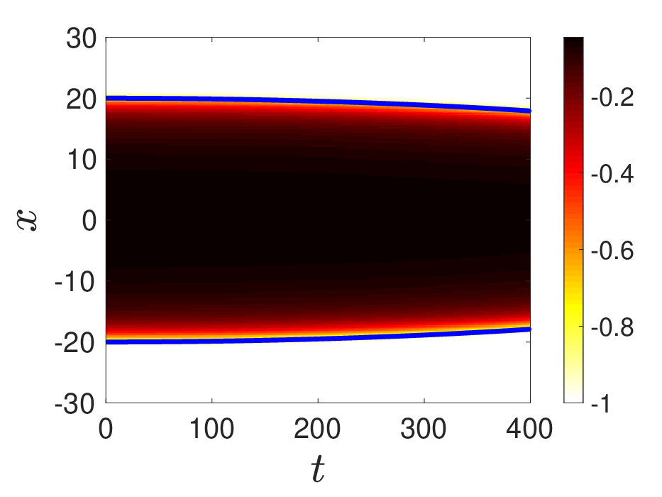
Next, consider what happens when we use Eq. (29) to create initial conditions for a prototypical kink-antikink collision simulation. We restrict ourselves to the case in which the kink and antikink are initially stationary, i.e., $v=0$; we do this to avoid the complication(s) of how an initial kinetic energy may affect the dynamics. In Fig. 2(a), we show a contour plot of the space-time evolution of the PDE solution, $\varphi(x,t)$; superimposed onto the contour plot (in this an all subsequent figures) are the curves $x=x_{\mathrm{K}}(t)$ (the location of the kink’s center) and $x=x_{\mathrm{\bar{K}}}(t)$ (the location of the antikink’s center). In Fig. 2(b), we show a plot of the velocity of the kink as a function of time. Specifically, we define $x_{\mathrm{K}}$ (bottom bold curve in Fig. 2(a)) as the (approximate) intersection of $\varphi$ with $-0.83356=\varphi_{(-1,0)}(0)$. [Note that this is the $\varphi$-value of the single kink profile at $x=0$ with $x_{0}=0$.] The approximation is done through linear interpolation of the two points on the shape with the $\varphi$-values closest to $-0.83356$. Similarly, in $x_{\mathrm{\bar{K}}}$ (top bold curve in Fig. 2(a)) denotes the approximate intersection of $\varphi$ with $-0.83356=\varphi_{(0,-1)}(0)$. The velocity of the kink is calculated by using the formula $v(t_{i})=[x_{\mathrm{K}}(t_{i+1})-x_{\mathrm{K}}(t_{i-1})]/(t_{i+1}-t_{i-1})$, given the solution at three discrete time values $t_{i-1}$, $t_{i}$ and $t_{i+1}$ for any $i$.

Earlier work Belendryasova.arXiv.08.2017 has suggested that a repulsive force might exists between the example kink and antikink considered above. Yet, we argue that this apparent repulsion is a result of the ansatz selected in Eq. (29) being a poor quantitative approximation of a kink-antikink solution. Recall the undershoot below $\varphi=-1$ near $x=\pm 20$ in Fig. 1. We can think of this undershoot as providing a kind of initial “spring board,” which pushes the “points” just above the spring board upward, and consequently causes the kink to move to the left and the antikink to move to the right. Furthermore, this upward motion creates disturbances at $x\approx\pm 20$ that move upwards and then along the top of the kink-antikink combination until they meet at $x=0$. One can see these effects clearly in the contour plot in Fig. 2(a). One can also see that, after meeting at $x=0$, these disturbances are trapped between the centers of the kink and antikink, which they reach again just before $t=50$. From the plot of the kink velocity in Fig. 2(b), it is clear that just at this time the arrival of the disturbance gives another boost to the velocity of the kink in the negative direction. Again, the disturbances are reflected back towards $x=0$ and out again to the centers of the kink and antikink for another boost to the velocities, pushing them apart faster. This phenomenology holds for other values of the initial half-separation $x_{0}$, down to $x_{0}=2.5$.

Thus, we have accounted for the apparent repulsive force, in the long-range interaction between a $\varphi^{8}$ kink and antikink, by showing that this “force” is simply the result of initial conditions that have been derived from an inaccurate sum ansatz. More specifically, we have quantified how this ansatz does not lead to a sufficiently accurate description of the motion of a kink-antikink pair. An additional (albeit weaker) effect along this vein consists of the radiative wavepackets, emitted from each kink, that affect both of them in the process.

A steady-state solution of Eq. (4) satisfies $-\partial^{2}\varphi/\partial x^{2}+V^{\prime}(\varphi)=0$. The last equation can be discretized as $-D_{2}\varphi+V^{\prime}(\varphi)$, where $D_{2}$ is again the pseudospectral differentiation matrix as in trefethen, on $N$ discrete and equally spaced $x$ and $\varphi$ values. Furthermore, we want the initial positions of the two topological solitons (given by $-x_{0}$ and $x_{0}$) to have specified values, which adds two more discrete equations (for a total of $N+2$). These two additional equations are $\varphi(-x_{0})-\tilde{\varphi}=0$ and $\varphi(x_{0})-\tilde{\varphi}=0$, where $\tilde{\varphi}$ is the $\varphi$ value of a single kink or antikink at $x=0$. The resulting set of equations is over-determined and has no solution.

As a remedy, we propose to improve the initial conditions introduced in the previous section by employing Eq. (29) as the initializer for a weighted nonlinear least-squares minimization of the objective function

$$\mathcal{I}[\varphi]=\left\|-D_{2}\varphi+V^{\prime}(\varphi)\right\|_{2}^{2}+C\left|\varphi(-x_{0})-\tilde{\varphi}\right|^{2}+C\left|\varphi(x_{0})-\tilde{\varphi}\right|^{2},$$

(30)

where $\|\cdot\|_{2}$ is the usual Euclidean norm, and $C$ is an empirical constant. Then, we can use the minimizer $\varphi_{\min}(x)$ of $\mathcal{I}$ as the initial condition for a direct numerical simulation of kink-antikink collisions, ensuring that our initial condition quantitatively satisfies the PDE to some preset accuracy. We take $C=50$, which is sufficient to keep the initial kink and antikink locations nearly fixed at $\pm x_{0}$ during the minimization process. The optimization problem is solved using MATLAB’s optimization toolkit, specifically via the lsqnonlin subroutine.

In Fig. 3, for $x_{0}=20$, we compare the sum ansatz from Eq. (29) (in dark blue) with the minimizer $\varphi_{\min}(x)$ of $\mathcal{I}$ (light blue). Specifically, note that we no longer observe the undershoot below $\varphi=-1$ in the plot of the minimized function. Additionally, $\varphi_{\min}(x)$ comes closer to $\varphi=0$ near $x=0$. Table 1 shows a more detailed quantitative comparison of $maxAbsPde$ for the minimized and (non-minimized) sum ansätze. Specifically, the maximum value of $maxAbsPde$ when taking $\varphi=\varphi_{\min}(x)$ is several orders of magnitude smaller than when using the sum ansatz from Eq. (29). Thus, we conjecture that the initial conditions generated from $\varphi_{\min}(x)$ will more accurately reflect the actual kink-antikink solution of this non-integrable field theory, at least considerably better than the non-minimized sum ansatz from Eq. (29).

To support our conjecture, Fig. 4 shows the result of a direct numerical simulation of the PDE (4), for our $\varphi^{8}$ model, using the minimized function $\varphi_{\min}(x)$ to generate the initial conditions. As before, this simulation corresponds to a kink-antikink interaction with $v=0$ because $\varphi_{\min}(x)$ approximates a stationary solution of the PDE. As in Fig. 2, we show both a contour space-time plot and a velocity plot in Fig. 4. Now, we observe an attractive force between the kink and antikink. Also, there are no visibly discernible small disturbances moving back and forth between $x=\pm 20$. This example simulation, along with numerous other similar simulations for different $x_{0}$ values, suggest that we have eliminated the significant detrimental effects of the algebraic kink and antikink tails (and of radiation), and we can thus now observe the proper (effective) inter-particle interaction between the kink and antikink. Also, note that this interaction is more in line with what one would naturally expect from a PDE of the type in Eq. (4), in that the $\partial^{2}\varphi/\partial x^{2}$ term tends to “pull points down” (pulling the kink and antikink together) when the function is concave down. Finally, the minimized ansatz $\varphi_{\min}(x)$ serves not only as an initial condition for the PDE simulations, but also as an appropriate ansatz for the collective coordinates approach described in the Appendix.

Besides finding $\varphi$ such that $\mathcal{I}$ in Eq. (30) is minimized, there are other possible setups that could be used to generate initial conditions for direct numerical simulation of the PDE (4) (and possibly for collective coordinate approaches as well). For example, one can use a product (rather than a sum) ansatz. Such an ansatz, customized for our $\varphi^{8}$ model, is

$$\varphi(x,t)=\left[\varphi_{(-1,0)}\left(\frac{x+x_{0}-vt}{\sqrt{1-v^{2}}}\right)+1\right]\left[\varphi_{(0,-1)}\left(\frac{x-x_{0}+vt}{\sqrt{1-v^{2}}}\right)+1\right]-1,$$

(31)

which we term the product ansatz.

Numerical simulations starting from Eq. (31) as an initial condition (again with $v=0$), once again exhibit a repulsion initially (though, weaker than for the sum ansatz) for $x_{0}>x_{c}$ where $6.2<x_{c}<6.3$. For $x_{0}<x_{c}$, attraction is found in the direct numerical simulations. Figure 5 shows the contour and the velocity plots for $x_{0}=6.2$, which leads to attraction, and for $x_{0}=6.3$, which leads to repulsion, having used the product ansatz in Eq. (31) to generate the initial conditions. In other words, the product ansatz creates the illusion of a possible saddle point configuration near $x_{0}=x_{c}$, such that attraction ensues for smaller (and repulsion for larger) initial sperations between the kink and the antikink. Minimization can be applied to the product ansatz from Eq. (31) as well, along the lines of Sec. III.3. The results are similar to those corresponding to using the minimized sum ansatz; in fact, the resulting minimized functions are nearly identical. Naturally, the output of this procedure decreases the undershoot from $-1$ (admittedly weaker with the product ansatz than with the sum ansatz) and passes even closer to $\varphi=0$ in the vicinity of $x=0$; see Fig. 6. Minimizing the product ansatz also leads to generic attraction, as we have come to expect, at this point, from the $\varphi^{8}$ field theory. All of these observations are illustrated in Fig. 7.

A third option is to treat the kink and antikink “completely separately,” meaning to use the kink formula for $x<0$ and the antikink formula for $x\geq 0$. To accomplish such a feat, we define

$$\varphi(x,t)=[1-H(x)]\varphi_{(-1,0)}\left(\frac{x+x_{0}-vt}{\sqrt{1-v^{2}}}\right)+H(x)\varphi_{(0,-1)}\left(\frac{x-x_{0}+vt}{\sqrt{1-v^{2}}}\right),$$

(32)

which we term the split-domain ansatz. Here, $H(x)$ is the Heaviside unit-step function. Using this ansatz to generate the initial conditions for a PDE simulation, we plot the contours of $\varphi$ and the kink velocity for $x_{0}=6.2$ and $x_{0}=6.3$ in Fig. 8. Contrary to what was the case for the product ansatz, we observe attraction for both $x_{0}$ values. It is perhaps natural to expect that the split-domain ansatz is the most accurate unminimized one (i.e., among the more standard ones that have not been “optimized” via our proposed minimization procedure), but it is expected to be limited in accuracy in the vicinity of $x=0$ due to the derivative discontinuity introduced in Eq. (32). This observation is substantiated by the kink-antikink dynamics shown in Fig. 8.

In this case, the ansatz is continuous at $x=0$ but its first derivative is not. The minimized version for the split-domain ansatz is quite similar to the non-minimized version; the “point” created where the kink and antikink meet at $x=0$ (due to the discontinuity in the derivative) is smoothed by the minimization procedure, but the two look rather similar otherwise. Figure 9 shows how the minimized version of the split-domain ansatz differs from its non-minimized counterpart. The dynamics of the split-domain ansatz comes closest to the minimized case in that it generically leads to attraction of the kink and antikink.

One other property of the various ansätze that is worth mentioning is the relative smoothness of the velocity graphs. One sees significant oscillations in the velocity of the center of the kink (or antikink) for all of the non-minimized ansätze (see, e.g., Fig. 2). The minimized versions of all three ansätze, on the other hand, show a steadily increasing velocity function (see, e.g., Fig. 4).

In Table 2, we show a comparison of the minimized versus non-minimized values of the PDE residual, $maxAbsPde$, for the product and split-domain ansätze. Note that for the non-minimized split domain case, $\partial^{2}\varphi/\partial x^{2}$ is not defined due to the discontinuity in the derivative at $x=0$, and hence the value of $maxAbsPde$ is listed as NA (“not available”). Another reason as to why we have elected not to provide this value is that the ansatz was constructed from the (numerically evaluated) exact solution of the BPS equation (no minimization) for each $x>0$ and $x<0$, which already satisfy $maxAbsPde=0$ numerically. Figure 10 shows the equivalent plots of those in Fig. 2 (non-minimized sum ansatz) and Fig. 4 (minimized sum ansatz) for the split-domain ansatz from Eq. (32).

A plot giving a sense of how the initial conditions for the $\varphi^{8}$ model compare for the different ansätze is shown in Fig. 11 for $x_{0}=4.5$ and $v=0$. We observe that all minimized ansätze lie between the sum/product and the split-domain ansatz. Interestingly, the results of the different minimization procedures are close to each other functionally, and the differences between them are difficult to detect without zooming in.

To summarize: our results indicate that the correct interpretation of the nature of the pairwise kink-antikink interaction is that the kink and antikink attract each other. We proposed the minimization procedure in Sec. III.3 as a way to “distill” the initial data and, thus, observe the genuine interaction dynamics of the kink and antikink without the detrimental side effects of the undershoot caused by their tails, as well as the radiation caused by the inexact initial conditions. While it is impossible to push the objective functional $\mathcal{I}$ from Eq. (30) to zero exactly (due to the absence of multi-soliton solutions for such a non-integrable model), the minimization of $\mathcal{I}$ brings the initial $\varphi$ field as close as possible to a distilled configuration involving the superposition of a kink and an antikink. On the other hand, in the absence of access to such a minimization procedure, our recommendation is to use the split-domain ansatz from Eq. (32) directly, as it is the one that bears the least spurious byproducts among the “standard” multi-soliton ansätze, even though it introduces a derivative discontinuity at $x=0$.

We find similar behaviors when considering ansätze for the corresponding $\varphi^{10}$ and $\varphi^{12}$ field theories with three degenerate minima. In particular, we considered the models represented by the potentials $V(\varphi)=\varphi^{6}(1-\varphi^{2})^{2}$ (khare, Sec. IV D.3) and $V(\varphi)=\varphi^{8}(1-\varphi^{2})^{2}$ (khare, Sec. IV D.1), respectively. These examples come from the systematic classification of higher-order field theory potentials with degenerate minima khare for which exact (albeit implicit) kink solutions are possible. Using the methodology introduced in Sec. II.1, it can be shown that these potentials satisfy the conditions for the existence of kinks with power-law tails. More specifically, a kink of the model $\varphi^{10}$ potential above approaches $-1$ exponentially as $x\rightarrow-\infty$, but approaches $0$ as $k/x^{1/2}$ (for some $k$ constant) when $x\rightarrow+\infty$. Similarly, a kink of the model $\varphi^{12}$ potential above approaches $-1$ exponentially as $x\rightarrow-\infty$, but approaches $0$ as $k/x^{1/3}$ (for some $k$ constant) when $x\rightarrow+\infty$. Thus, these higher-order field theory models possess solutions with “fatter” tails.

Table 3 shows the $maxAbsPde$ residuals for the $\varphi^{10}$ model in a way that parallel Tables 1 and 2 for the $\varphi^{8}$ case. Table 4 shows the equivalent results for the $\varphi^{12}$ model. We observe similar trends for these models to what we saw in the $\varphi^{8}$ case; once again, the minimization procedure significantly improves the quantitative agreement between an initial condition ansatz profile and a hypothetical one that exactly satisfies the PDE (4).

Though the contour and velocity plots for the $\varphi^{10}$ and $\varphi^{12}$ models are generally quite similar to the $\varphi^{8}$ plots for many cases, we point out a few cases in which the collisions in the higher-order field theories differ. Primarily, the differences occur for the non-minimized sum ansatz, for which we find that the initial conditions chosen based on this ansatz do not lead to clearly attracting or repelling kink-antikink pairs, for certain values of $x_{0}$. Rather, for these cases, the ansatz leads to solutions that show oscillations in the range $\varphi=-1$ to $\varphi=1$ rather than topological solitons connecting $\varphi=-1$ to $\varphi=0$.

A way to explain this strange result is to consider the fact that for such fatter-tail cases, as the ones arising from the example $\varphi^{10}$ and $\varphi^{12}$ field theories considered herein, the undershoot of the kinks is so substantial that not only is the $\varphi=0$ fixed point not reached between the kinks, but also neither is the asymptotic value of $\varphi=-1$ as $|x|\gg 1$. In other words, the (non-minimized) sum ansatz provides an extremely poor initial conditions for the fatter-tail cases.

We can obtain some further insight into this quantitative disagreement by considering the graphs of the sum ansatz for the three cases; see Fig. 12 ($\varphi^{8}$ on top, $\varphi^{10}$ in middle, and $\varphi^{12}$ at the bottom). The “fat tails” of the $\varphi^{12}$ kink give such a large boost to the points in the middle (springboard effect) that they travel past the potential minimum at $\varphi=0$ to the neighborhood of $\varphi=1$ under the evolution of the PDE (4). This effect persists for $x_{0}=5$, $10$, $20$, $50$ and $100$ for the $\varphi^{12}$ model (recall Table 4), and to a lesser extent for $x_{0}=5$, $10$ and $20$ for the $\varphi^{10}$ model (recall Table 3). In all of these cases, the notions of “attracting kinks” and “repelling kinks” are no longer meaningful.

References

- (1) A. Vilenkin and E. P. S. Shellard, Cosmic Strings and Other Topological Defects (Cambridge University Press, Cambridge, 2000).
- (2) N. Manton, P. Sutcliffe, Topological Solitons (Cambridge University Press, Cambridge, 2004).
- (3) V. V. Kiselev, Collective Effects in Condensed Matter Physics (de Gruyter, Berlin, 2018)
- (4) A. R. Bishop, J. A. Krumhansl, and S. E. Trullinger, Solitons in condensed matter: A paradigm, Physica D 1, 1 (1980).
- (5)
(a) L. D. Landau, Theory of Phase Transitions. I (in Russian), Zh. Eksp. Teor. Fiz. 7, 19 (1937);
(b) V. L. Ginzburg and L. D. Landau, Theory of Superconductivity (in Russian), Zh. Eksp. Teor. Fiz. 20, 1064 (1950). - (6) M. Tinkham, Introduction to Superconductivity (McGraw-Hill, New York, 1996).
- (7) D. K. Campbell, J. F. Schonfeld, and C. A. Wingate, Resonance structure in kink-antikink interactions in theory, Physica D 9, 1 (1983).
- (8) A. Khare, I. C. Christov, and A. Saxena, Successive phase transitions and kink solutions in , , and field theories, Phys. Rev. E 90, 023208 (2014) [arXiv:1402.6766].
- (9) Y. M. Gufan and E. S. Larin, Dokl. Akad. Nauk SSSR 242, 1311 (1978) [Phenomenological analysis of isostructural phase transitions, Sov. Phys. Dokl. 23, 754 (1978)].
- (10) A. Saxena, I. C. Christov, A. Khare, “Higher-order field theories: , and beyond,” in: A dynamical perspective on the model: Past, present and future, eds. P. G. Kevrekidis and J. Cuevas-Maraver, Chap. 11 (Springer-Verlag, Heidelberg, 2019) [arXiv:1806.06693].
- (11)
(a) D. Bazeia and F. S. Bemfica, From Supersymmetric quantum mechanics to scalar field theories, Phys. Rev. D 95, 085008 (2017) [arXiv:1703.00277];
(b) D. Bazeia and F. S. Bemfica, From scalar field theories to supersymmetric quantum mechanics, Mod. Phys. Lett. A 32, 1750073 (2017) [arXiv:1611.07106]. - (12) D. Castañeda Valle and E. W. Mielke, Relativistic soliton collisions of axion type dark matter, Phys. Lett. B 758, 93 (2016).
- (13) E. Greenwood, E. Halstead, R. Poltis, and D. Stojkovic, Electroweak vacua, collider phenomenology, and possible connection with dark energy, Phys. Rev. D 79, 103003 (2009) [arXiv:0810.5343].
- (14) R. Poltis, Gravity waves seeded by turbulence and magnetic fields from a first order phase transition with non-renormalizable electroweak vacua [arXiv:1201.6362].
- (15) A. Arancibia, F. Correa, V. Jakubsky, J. Mateos Guilarte, and M. S. Plyushchay, Soliton defects in one-gap periodic system and exotic supersymmetry, Phys. Rev. D 90, 125041 (2014) [arXiv:1410.3565].
- (16) A. Arancibia and M. S. Plyushchay, Chiral asymmetry in propagation of soliton defects in crystalline backgrounds, Phys. Rev. D 92, 105009 (2015) [arXiv:1507.07060].
- (17) J. Mateos Guilarte and M. S. Plyushchay, Perfectly invisible -symmetric zero-gap systems, conformal field theoretical kinks, and exotic nonlinear supersymmetry, JHEP 2017 (12), 061 (2017) [arXiv:1710.00356].
- (18) O. DeWolfe, D. Z. Freedman, S. S. Gubser, and A. Karch, Modeling the fifth dimension with scalars and gravity, Phys. Rev. D 62, 046008 (2000) [hep-th/9909134].
- (19) T. Vachaspati, Kinks and Domain Walls: An Introduction to Classical and Quantum Solitons (Cambridge University Press, Cambridge, 2006).
- (20)
(a) D. K. Campbell and M. Peyrard, Solitary wave collisions revisited, Physica D 18, 47 (1986);
(b) D. K. Campbell, M. Peyrard, and P. Sodano, Kink-antikink interactions in the double sine-Gordon equation, Physica D 19, 165 (1986). - (21) P. Anninos, S. Oliveira, and R. A. Matzner, Fractal structure in the scalar theory, Phys. Rev. D 44, 1147 (1991).
- (22) R. H. Goodman and R. Haberman, Kink-Antikink Collisions in the Equation: The -Bounce Resonance and the Separatrix Map, SIAM J. Appl. Dyn. Sys. 4, 1195 (2005).
- (23) P. Dorey, K. Mersh, T. Romanczukiewicz, and Y. Shnir, Kink-antikink collisions in the model, Phys. Rev. Lett. 107, 091602 (2011) [arXiv:1101.5951].
- (24) R. H. Goodman, A. Rahman, M. J. Bellanich, and C. N. Morrison, A mechanical analog of the two-bounce resonance of solitary waves: Modeling and experiment, Chaos 25, 043109 (2015) [arXiv:1503.08315]
- (25) V. A. Gani, A. E. Kudryavtsev, and M. A. Lizunova, Kink interactions in the (1+1)-dimensional model, Phys. Rev. D 89, 125009 (2014) [arXiv:1402.5903].
- (26) H. Weigel, Kink-antikink scattering in and models, J. Phys. Conf. Series 482, 012045 (2014) [arXiv:1309.6607].
- (27) I. Takyi and H. Weigel, Collective Coordinates in one-dimensional soliton models revisited, Phys. Rev. D 94, 085008 (2016) [arXiv:1609.06833].
- (28) F. C. Simas, A. R. Gomes, K. Z. Nobrega, and J. C. R. E. Oliveira, Suppression of two-bounce windows in kink-antikink collisions, JHEP 2016 (09), 104 (2016) [arXiv:1605.05344].
- (29) A. Moradi Marjaneh, V. A. Gani, D. Saadatmand, S. V. Dmitriev, and K. Javidan, Multi-kink collisions in the model, JHEP 2017 (07), 028 (2017) [arXiv:1704.08353].
- (30) A. Demirkaya, R. Decker, P. G. Kevrekidis, I. C. Christov, and A. Saxena, Kink dynamics in a parametric system: A model with controllably many internal modes, JHEP 2017 (12), 071 (2017) [arXiv:1706.01193].
- (31)
(a) T. Romańczukiewicz, Could the primordial radiation be responsible for vanishing of topological defects?, Phys. Lett. B 773, 295 (2017) [arXiv:1706.05192];
(b) P. Dorey and T. Romańczukiewicz, Resonant kink–antikink scattering through quasinormal modes, Phys. Lett. B 779, 117 (2018) [arXiv:1712.10235]. - (32) M. A. Lohe, Soliton structures in , Phys. Rev. D 20, 3120 (1979).
- (33)
(a) D. Bazeia, M. A. González León, L. Losano and J. Mateos Guilarte, Deformed defects for scalar fields with polynomial interactions, Phys. Rev. D 73, 105008 (2006) [hep-th/0605127];
(b) D. Bazeia, M. A. González León, L. Losano, J. Mateos Guilarte, New scalar field models and their defect solutions, EPL 93, 41001 (2011) [arXiv:1101.5102];
(c) D. Bazeia, M. A. González León, L. Losano, J. Mateos Guilarte, J. R. L. Santos, Construction of new scalar field models from the standard theory, Phys. Scr. 87, 045101 (2013) [arXiv:1302.6032]. - (34) A. R. Gomes, R. Menezes, and J. C. R. E. Oliveira, Highly interactive kink solutions, Phys. Rev. D 86, 025008 (2012) [arXiv:1208.4747].
- (35) V. A. Gani, V. Lensky, and M. A. Lizunova, Kink excitation spectra in the (1+1)-dimensional model, JHEP 2015 (08), 147 (2015) [arXiv:1506.02313].
- (36) V. A. Gani, V. Lensky, M. A. Lizunova, and E. V. Mrozovskaya, Excitation spectra of solitary waves in scalar field models with polynomial self-interaction, J. Phys.: Conf. Ser. 675, 012019 (2016) [arXiv:1602.02636].
- (37) R. V. Radomskiy, E. V. Mrozovskaya, V. A. Gani, and I. C. Christov, Topological defects with power-law tails, J. Phys. Conf. Ser. 798, 012087 (2017) [arXiv:1611.05634].
- (38) E. Belendryasova and V. A. Gani, Resonance phenomena in the kinks scattering, J. Phys.: Conf. Ser. 934, 012059 (2017) [arXiv:1712.02846].
- (39) E. Belendryasova and V. A. Gani, Scattering of the kinks with power-law asymptotics, Commun. Nonlinear Sci. Numer. Simulat. 67, 414 (2019) [arXiv:1708.00403].
- (40) D. J. Kaup and A. C. Newell, An exact solution for a derivative nonlinear Schrödinger equation, J. Math. Phys. 19, 798 (1977).
- (41) M. J. Ablowitz and J. Satsuma, Solitons and rational solutions of nonlinear evolution equations, J. Math. Phys. 19, 2180 (1977).
- (42) D. Bazeia, R. Menezes, and D. C. Moreira, Analytical study of kinklike structures with polynomial tails, J. Phys. Commun. 2, 055019 (2018) [arXiv:1805.09369].
- (43) T. Sugiyama, Kink-antikink collisions in the two-dimensional model, Prog. Theor. Phys. 61, 1550 (1979).
- (44) T. I. Belova and A. E. Kudryavtsev, Solitons and their interactions in classical field theory, Phys. Usp. 40, 359 (1997) [Usp. Fiz. Nauk 167, 377 (1997)].
- (45) H. E. Baron, G. Luchini, and W. J. Zakrzewski, Collective coordinate approximation to the scattering of solitons in the (1+1) dimensional NLS model, J. Phys. A: Math. Theor. 47, 265201 (2014) [arXiv:1308.4072].
- (46) B. A. Malomed, Variational methods in nonlinear fiber optics and related fields, Prog. Opt. 43, 71 (2002).
- (47) D. Berenstein, Giant gravitons: A collective coordinate approach, Phys. Rev. D 87, 126009 (2013) [arXiv:1301.3519].
- (48) H. Hata and T. Kikuchi, Relativistic Collective coordinate system of solitons and spinning Skyrmion, Prog. Theor. Phys. 125, 59 (2011) [arXiv:1008.3605].
- (49) K. Javidan, Collective coordinate variable for soliton-potential system in sine-Gordon model, J. Math. Phys. 51, 112902 (2010) [arXiv:0910.3058].
- (50) Ya. Shnir, Collective coordinates of the Skyrme model coupled with fermions, Phys. Scr. 67, 361 (2003) [hep-th/0307277].
- (51) B. A. Mello, J. A. González, L. E. Guerrero, and E. López-Atencio, Topological defects with long-range interactions, Phys. Lett. A 244, 277 (1998).
- (52) L. E. Guerrero, E. López-Atencio, and J. A. González, Long-range self-affine correlations in a random soliton gas, Phys. Rev. E 55, 7691 (1997).
- (53) J. A. González and J. Estrada-Sarlabous, Kinks in systems with degenerate critical points, Phys. Lett. A 140, 189 (1989).
- (54) N. S. Manton, An effective Lagrangian for solitons, Nucl. Phys. B 150, 397 (1979).
- (55) J. K. Perring and T. H. R. Skyrme, A model unified field equation, Nucl. Phys. 31, 550 (1962).
- (56) R. Rajaraman, Intersoliton forces in weak-coupling quantum field theories, Phys. Rev. D 15, 2866 (1977).
- (57) P. G. Kevrekidis, A. Khare, and A. Saxena, Solitary wave interactions in dispersive equations using Manton’s approach, Phys. Rev. E 70, 057603 (2004) [nlin/0410045].
- (58) N. S. Manton, Force between kinks with long-range tails [arXiv:1810.00788].
- (59) N. S. Manton, Force between Kink and Antikink with Long-range Tails [arXiv:1810.03557].
- (60) V. A. Gani and A. E. Kudryavtsev, Kink-antikink interactions in the double sine-Gordon equation and the problem of resonance frequencies, Phys. Rev. E 60, 3305 (1999) [cond-mat/9809015].
- (61) D. Bazeia, E. Belendryasova, and V. A. Gani, Scattering of kinks in a non-polynomial model, J. Phys.: Conf. Ser. 934, 012032 (2017) [arXiv:1711.07788].
- (62) D. Bazeia, E. Belendryasova, and V. A. Gani, Scattering of kinks of the sinh-deformed model, Eur. Phys. J. C 78, 340 (2018) [arXiv:1710.04993].
- (63) V. A. Gani, A. Moradi Marjaneh, A. Askari, E. Belendryasova, and D. Saadatmand, Scattering of the double sine-Gordon kinks, Eur. Phys. J. C 78, 345 (2018) [arXiv:1711.01918].
- (64)
(a) E. B. Bogomolny, Yad. Fiz. 24, 861 (1976) [Stability of classical solutions, Sov. J. Nucl. Phys. 24, 449 (1976)];
(b) M. K. Prasad and C. M. Sommerfield, Exact classical solution for the ’t Hooft monopole and the Julia-Zee Dyon, Phys. Rev. Lett. 35, 760 (1975). - (65) L. N. Trefethen, Spectral Methods in Matlab (Society for Industrial and Applied Mathematics, Philadelphia, PA, 2000).
- (66) I. C. Christov, R. J. Decker, A. Demirkaya, V. A. Gani, P. G. Kevrekidis, A. Khare, and A. Saxena, Kink-kink and kink-antikink interactions with long-range tails [arXiv:1811.07872].
- (67)
(a) A. Weller, J. P. Ronzheimer, C. Gross, J. Esteve, M. K. Oberthaler, D. J. Frantzeskakis, G. Theocharis, and P. G. Kevrekidis, Experimental Observation of Oscillating and Interacting Matter Wave Dark Solitons, Phys. Rev. Lett. 101, 130401 (2008) [arXiv:0803.4352];
(b) G. Theocharis, A. Weller, J. P. Ronzheimer, C. Gross, M. K. Oberthaler, P. G. Kevrekidis, and D. J. Frantzeskakis, Multiple atomic dark solitons in cigar-shaped Bose-Einstein condensates, Phys. Rev. A 81, 063604 (2010) [arXiv:0909.2122]. - (68) C. Becker, S. Stellmer, P. Soltan-Panahi, S. Dörscher, M. Baumert, E.-M. Richter, J. Kronjäger, K. Bongs, K. Sengstock, Oscillations and interactions of dark and dark-bright solitons in Bose–Einstein condensates, Nat. Phys. 4, 496 (2008) [arXiv:0804.0544].
Appendix: Collective Coordinate Approach and Connection to the Numerical Results
In this Appendix, we apply the method of collective coordinates (CC) using the minimized initial condition ansätze, which we introduced in the main text above to analyze the kink-antikink interactions numerically. To this end, recall that the Lagrangian for our neutral scalar field theories is