Sharp threshold phenomena in statistical physics
Abstract
This text describes the content of the Takagi lectures given by the author in Kyoto in 2017. The lectures present some aspects of the theory of sharp thresholds for boolean functions and its application to the study of phase transitions in statistical physics.
1 Introduction
In physics, a phase transition is a discontinuous change of behavior in a physical system as some of its parameters (for instance the temperature, the density or the pressure) vary continuously. The most classical examples are probably the transitions between solid, liquid and gaseous states of matter, and the transition from a ferromagnet to a paramagnet at Curie’s temperature, but physics offers many examples of phase transitions, whose understanding is crucial both theoretically and practically.
As an illustration for what will come next in these lectures, let us present the phase transition in a specific model for porous media called Bernoulli percolation. Consider the square lattice with vertex-set given by points of with integer coordinates, and edge-set given by pairs with ( is the Euclidean norm). Define the random graph, introduced by Broadbent and Hammersley in [10], obtained by keeping each edge of with probability (therefore erasing it with probability ) independently of the other edges. The large scale properties of the random graph constructed like that change drastically at a critical value of the parameter . More precisely, there exists such that
- •
If , the probability that there is an infinite connected component is zero.
- •
If , the probability that there is an infinite connected component is one.
(Note that we do not say anything about the case .) This is an archetypal example of a phase transition in statistical physics: as the parameter (which can be interpreted as density) is varied continuously through the value , the probability of having an infinite connected component jumps from 0 to 1.
It was conjectured early that the value of the critical point is equal to , but proving this statement took more than twenty years. One of the goals of these lectures is to provide a modern proof of this statement, based on the notion of sharp threshold.
In mathematics, a finite random system undergoes a sharp threshold if its qualitative behavior changes quickly as the result of a small perturbation of the parameters ruling the probabilistic structure. A fundamental example is provided by sharp thresholds undergone by the averages of boolean functions with respect to a product measure. More formally, for , let be the law of a sequence of iid Bernoulli random variables with parameter . In a slight abuse of notation, we will identify with its restriction to the first random variables when considering a boolean function . An element of will generically be denoted by . For future reference, we denote the set by . We will also write (and by extension if we consider a sequence of boolean functions ).
Definition 1.1
A sequence of increasing11 1 With respect to the standard partial ordering on : if for every . boolean functions undergoes a sharp threshold at if there exists tending to 0 such that and
The notion of sharp threshold emerged in the combinatorics community studying graph properties of random graphs. In [23], Erdös and Renyi introduced a model of random graph with vertex-set and edge-set , where is the set of pairs of integers in , which is identified with the set with to enter in our framework to define the measure as a product of Bernoulli. The authors were originally interested in graph properties of , i.e. properties of graphs that depend only on their isomorphism class22 2 Isomorphism class is understood for the equivalence via graph isomorphisms. More formally, consider two graphs and , with and the vertex-sets and and the edge-sets. A map is a graph isomorphism between and if it is bijective and if if and only if .. They first focused on two specific properties, described below,
Example 1: Connectivity of the graph
Erdös and Rényi [23] proved that if is the event that the graph is connected, then undergoes a sharp threshold at .
Example 2: Existence of a giant connected component
Later, Erdös and Rényi also proved that if denotes the existence of a component in of size larger or equal to , where the sequence satisfies and , then undergoes a sharp threshold at .
Since this seminal paper, many other graph properties have been studied, including existence of certain induced subgraphs, etc. In fact, it was shown later (we will justify this in the next section) that many graph properties undergo sharp thresholds, namely the monotonic properties (examples include being Hamiltonian, being non-planar, containing a clique of size , having a diameter smaller than , etc)
Example 3: Monotonic properties
Every sequence of increasing graph properties undergoes a sharp threshold with .
Let us remark that properties not undergoing a sharp threshold must essentially depend on a (uniformly) bounded number of bits.
When considering systems from statistical physics, the notion of sharp threshold often corresponds to a finite version of the notion of phase transition. In these lectures, we propose to start from the mathematical theory of sharp thresholds and explain how this theory sheds some new light on the understanding of phase transitions in statistical physics.
Section 3 presents two theorems from the study of boolean functions on product spaces. Section 4 discusses two applications to sharp phase transitions in statistical physics. Finally, Section 5 presents generalizations and applications of the theory of sharp thresholds for boolean functions to monotonic measures.
2 How to prove that a sequence of boolean functions undergoes a sharp threshold?
2.1 The Margulis-Russo differentiation formula
Let us start the study of averages of boolean functions by giving an expression for their derivatives. For a boolean function , introduce the notation , where is the configuration obtained by flipping the state of , i.e. more formally
The influence of :
Note that the influence depends on even though we do not refer to it in the notation.
Proof
Set . Differentiating with respect to immediately gives
| (2.1) |
Note that conditioned on , then is (conditionally) independent of and its (conditional) average in (2.1) is zero. Therefore,
For , the fact that is increasing implies that if , and if . We deduce that
Since and are independent, we conclude that
Inserting this expression in (2.1) implies the claim.
The previous lemma immediately gives that is increasing and differentiable. Therefore, if one can prove bounds of the type
| (2.2) |
for some large constant , one deduces that the window of values of for which remains far from and is necessarily small. Indeed, since takes values in , we find
which, together with Lemma 2.1, enables one to rewrite (2.2) as
Let be such that , then for any , integrating the previous differential inequality between and gives . Similarly, integrating the differential inequality between and gives . In particular, this shows that for , one has and . The next sections are describing arguments leading to inequalities of the form of (2.2).
2.2 A sharp threshold inequality
Historically, the general theory of sharp thresholds for discrete product spaces was initiated by Russo in [37] and Kahn, Kalai and Linial in [31] in the case of the uniform measure on , i.e. to the case of with . There, Kahn, Kalai and Linial used the Bonami-Beckner inequality [2, 8] to deduce inequalities between the variance of a boolean function and influences of this function (Beckner proved a similar inequality for Gaussian measures). Bourgain, Kahn, Kalai, Katznelson and Linial [9] extended these inequalities to product spaces endorsed with the uniform measure (for which the Bonami-Beckner inequality does not hold). Then, a discretization scheme enables one to deduce sharp threshold results on for with arbitrary . Recently, the result was extended to any product space in [29]. Here, we state a theorem due to Talagrand [39] which is essentially equivalent to the BKKKL result [9] for what we have in mind.
Theorem 2.2 (Talagrand [39])
There exists a constant such that for any and , the following holds. For any increasing boolean function ,
This statement is often used as follows: there must necessarily exist one influence which is larger than (where ), which is immediate since there must be one with
(with maybe changed by a constant multiplicative factor).
Proof
The proof of this theorem is based on discrete Fourier analysis. Let us focus on the case which is slightly simpler due to the Bonami-Beckner inequality. We use the Fourier-Walsh expansion of
where and . Observe that
Since , and since by Parseval’s inequality, , we deduce that
We deduce that
Writing and introducing for each ,
we may write
where . We now use the Bonami-Beckner inequality [2, 8], which states that
Since takes values in , we also have that . We deduce that
| (2.3) |
Now, and , so making the change of variables gives
Plugging this inequality in (2.3) gives the result.
The whole gain in the previous proof comes from the Bonami-Beckner inequality. This inequality is not obvious to prove, and we refer to [2, 8] for details.
Note that this inequality implies that is much larger than as soon as all the influences are small (which can be seen counterintuitive since the derivative is the sum of the influences). More precisely, if all the influences are smaller than , then is larger than .
In general, it may be difficult to prove that all influences are small, but there is a particularly efficient way of using Theorem 2.2 when is invariant under a group acting transitively on .
Theorem 2.3
There exists such that for any and , the following holds. For an increasing boolean function which is symmetric33 3 Meaning that for every . under a group acting transitively on ,
Proof
Since the boolean function is symmetric under a group acting transitively on , we have that for each and , for any satisfying . In particular, we deduce that
and therefore all the influences are equal. Now, we are facing two cases:
- •
if for all , then
- •
if for all , then for all and Theorem 2.2 implies
By modifying and choosing it small enough, we obtain the result.
This theorem is already quite powerful since it guarantees that one may take . In particular, this theorem implies that every monotone graph property undergoes a sharp threshold (see Example 3 of the previous section). Indeed, by definition a graph property is invariant under graph isomorphism. In particular, it is invariant under relabeling of the vertices, and therefore is invariant under a group acting transitively on the vertices of the graph.
2.3 The O’Donnell-Schramm-Saks-Servedio inequality
We now present another inequality enabling to derive bounds like (2.2). This one is based on algorithms and was introduced to solve a conjecture of Yao [42].
Informally speaking, an algorithm associated with a boolean function takes as an input, and reveals algorithmically the value of at different coordinates one by one until the value of is determined. At each step, which coordinate will be revealed next depends on the values of revealed so far. The algorithm stops as soon as the value of is the same no matter the values of on the remaining coordinates. Then, the question is often to determine how many bits of information must be revealed before the algorithm stops (this quantity is sometimes referred to as the computational complexity of the boolean function).
Formally, an algorithm is defined as follows. For a -tuple and , write and . An algorithm takes as an input and gives back an ordered sequence constructed inductively as follows: for any ,
where is a function interpreted as the decision rule at time ( takes the location and the value of the bits for the first steps of the induction, and decides the next bit to query). Note that the first coordinate is deterministic. For , define
Remark 2.4
In computer science, an algorithm is usually associated directly to a boolean function and defined as a rooted directed tree in which each internal nodes are labeled by elements of , leaves by possible outputs of , and edges are in correspondence with the possible values of the bits at vertices (see [35] for a formal definition). In particular, the algorithms are usually defined up to , and not later on.
The OSSS inequality, originally introduced by O’Donnell, Saks, Schramm and Servedio in [35] as a step toward a conjecture of Yao [42], relates the variance of a boolean function to the influence and the computational complexity of an algorithm for this function.
Theorem 2.5 (OSSS inequality [35])
Consider and . Fix an increasing boolean function and an algorithm . We have
| (2.4) |
where is called the revealment of for the algorithm and the bit .
Proof
Consider two independent sequences and of iid Bernoulli random variables of parameter . Write for the joint measure of these variables (and for its expectation). Construct by setting and for , . Note that the construction of relies solely on and does not involve . Define
Finally, for , define
where it is understood that the -tuple under parentheses is equal to if .
Now, observe that takes values in , therefore
Since and coincide on , we deduce that . Also, so that . As a consequence, conditioning on gives
Since for any , the right-hand side is smaller than or equal to
We now use the key property of the construction of the . Conditionally on and , both and are independent sequences of iid Bernoulli random variables since both involve only on edges in . Furthermore, they differ (possibly) at since and . We insist on the fact that this is the fundamental property that we were looking for when defining . We deduce that
Recalling that concludes the proof.
3 Applications to Bernoulli percolation on
We now focus on two applications to Bernoulli percolation. Consider the -dimensional lattice with vertex set and edge set given by pairs with . We do not work on boolean functions defined on anymore but rather on with being a finite set. In particular, we will use the notation instead of to refer to elements of (which are all edges of ). Note that the theorems proved in the previous section are also valid in this context.
Set and . Also, set if there exists a path in from to . Finally, we write for the event that 0 is in an infinite connected component.
3.1 Critical point of Bernoulli percolation on
In this section, we discuss the proof of the following theorem.
Theorem 3.1 (Kesten [32])
The critical point of Bernoulli percolation on the square lattice is equal to .
We present a method initiated first by Russo [37]. It was later developed further by Bollobàs and Riordan [4, 5, BolRioc]. It is based on the existence of a sharp threshold for so-called crossing probabilities. For two integers and , define the rectangle . Consider the event to be events that the configuration contains a path in from the left side to the right side44 4 The left side is and the right side . We take this opportunity to also define the bottom side and the top side for future reference. of . In this case, we say that is crossed horizontally. Similarly, one defines to be the event that the configuration contains a path in from the bottom to the top of . In this case, we say that is crossed vertically.
Let us start by a simple observation.
Proposition 3.2
We have for all .
Proof
Consider the dual lattice of the lattice defined by putting a vertex in the middle of each face, and edges between nearest neighbors. Each edge is in direct correspondence with an edge of the dual lattice crossing it in its middle. For a finite graph , let be the graph with edge-set and vertex-set given by the endpoints of the edges in .
A configuration in is naturally associated with a dual configuration on as follows: for every , set . Note that if the law of is a product of independent Bernoulli variables with parameter , then the law of is a product of Bernoulli variables with parameter .
Observe that the complement of the event is the event that there exists a path of edges in going from top to bottom in the graph . Using the symmetry by rotation by , one sees that at , these two events have the same probability, which must therefore be equal, for every , so that
| (3.1) |
In particular, crossing probabilities for squares (they are not quite squares but it is pretty much the same) do not tend to 0 or 1 as tends to infinity. One may wonder whether this is simply due to the fact that we chose a rectangle which is almost a square, or whether this holds for every rectangle which is not too degenerate, meaning that they are not too flat. We are going to see that this is the case. This property, which is called the Box-Crossing Property, is absolutely fundamental for the understanding of the phase .
Theorem 3.3
For any , there exists such that for all ,
Note that we immediately deduce a similar bound for probabilities of being crossed vertically. The uniform upper bound follows easily from the uniform lower bound and duality since the complement of the event that a rectangle is crossed vertically is the event that the dual rectangle is crossed horizontally in the dual configuration.
Also, as soon as we have to our disposal a uniform lower bound (in ) for some , then one can easily combine crossings in different rectangles to obtain a uniform lower bound for any . Indeed, define (for every integer ) the rectangles and the squares . Also define and to be the events that is crossed horizontally, and vertically. Then,
| (3.2) |
Above, we used the following inequality, known as the Harris or FKG inequality (see [27]): for any two increasing boolean functions and ,
| (3.3) |
Note that for the event under consideration in (3.2), indication functions were increasing.
Unfortunately, we cannot start a priori from an estimate with and must deal with the case . This will in fact be the major obstacle: the main difficulty of Theorem 3.3 lies in passing from crossing squares with probabilities bounded uniformly from below to crossing rectangles in the hard direction with probabilities bounded uniformly from below. A statement claiming that crossing a rectangle in the hard direction can be expressed in terms of the probability of crossing squares is called a Russo-Seymour-Welsh type theorem. For Bernoulli percolation on the square lattice, such a result was first proved in [36, 38]. Since then, many proofs have been produced, among which [4, 6, 7, 41, 40]. This seemingly technical statement is in fact at the root of virtually every study of the critical phase of Bernoulli percolation.
Proof
As mentioned before the proof, it is sufficient to prove that the crossing probability in the hard direction, for a rectangle with :
We choose to work with vertical crossings of the rectangle . We will need some additional notation. Set and . Also, define to be the bottom side of (or equivalently of ).
Let (resp. ) be the event that there exists a bottom-top (left-right) crossing of , and be the event that there exists a left-right crossing of that is connected to in . For a path from left to right in , and the reflection of this path with respect to , define the set of vertices in below (see Fig. 2 on the left). Now, on , condition on the highest left-right crossing of . We find that
In the third line, to deduce the lower bound , we used the facts that conditioned on , the configuration in is a Bernoulli percolation of parameter (since is measurable with respect to the random variables for edges on or above ), the symmetry and the fact that the probability of a bottom-top crossing in is larger than (since it is easier than a bottom-top crossing of ). Fig. 2 on the right illustrates that is crossed vertically if the three events , and occur, where is the event that there exists a left-right crossing of which is connected to in . By symmetry,
The FKG inequality (3.3) (used in the second inequality) implies that

Note that a trivial corollary of the previous statement is the following.
Corollary 3.4
There exists such that for all , In particular, .
Proof
Consider the event that is connected to . For this event to happen, it is necessary that one of the four rotated versions of the event that is crossed vertically must occur. Therefore, the FKG inequality applied to the complements of these events implies that
Since is included in the intersection of the events that , where is a power of 2, the independence implies that
provided is chosen small enough.
To prove that , observe that by letting tends to infinity, we find that . Using that there are countably many vertices in , and that for each one of them, the probability of being connected to infinity is zero (by invariance under translations), we deduce that the probability that there is an infinite connected component in is 0.
Now that we proved that crossing probabilities remain bounded away from 0 and 1 at , it is natural to ask oneself whether this is also the case for the values of that are not equal to . This is where we will use Theorem 2.2. We will prove the following statement:
Proposition 3.5
For any , there exists such that .
Proof
Consider the boolean function . Fix an edge of and observe that if , then one of the endpoints of the dual edge of must be connected by a path in the dual configuration of to distance . Since is sampled according to iid Bernoulli random variables of parameter , Corollary 3.4 implies that
where . As a consequence, we deduce from Theorem 2.3 that for any ,
Integrating this differential inequality between and gives that
The result follows by setting small enough.
Proof of Theorem 3.1
We already know that . Let us prove the other inequality by proving that for , the probability that there exists an infinite connected component in is 1. Let and be the events of and respectively. Observe that if and occur for all but finitely many , then there exists an infinite connected component in .
The previous proposition implies that
so that the Borel-Cantelli lemma55 5 The Borel-Cantelli lemma states that if is a sequence of events such that , then the probability that there are infinite many such that occurs is zero. implies that the probability that occurs for all but finitely many is 1. By symmetry by rotation by an angle of , we immediately deduce the same for the events . In conclusion, we proved that the probability that there exists an infinite connected component in is 1.
3.2 Sharpness of the phase transition for Bernoulli percolation on
In higher dimensions, it is hopeless to try to compute the exact value of the critical point (one does not expect it to be equal to any nice number, for instance rational or even algebraic). Nonetheless, one can still try to prove that the model undergoes a sharp phase transition, meaning that probabilities to be connected to distance decay very fast when .
Theorem 3.6
Consider Bernoulli percolation on ,
- 1.
For , there exists such that for all , .
- 2.
There exists such that for , .
Note that the theorem does not mention anything on the phase. The reason is that the proof relies deeply on moving the value of . The question of the phase is tremendously difficult in general and we avoid discussing it here. Let us also mention that the second item is often called the mean field lower bound. The lower bound is matched (up to constant) for [24], but is expected not to be sharp for small values of (this fact is known in dimension 2).
Theorem 3.6 was first proved by Aizenman, Barsky [1] and Menshikov [34] (these two proofs are presented in [27]). See also a recent short proof [21, 22]. Here, we choose to present a new proof [18] using the OSSS inequality. Let us start the proof with a general lemma which is nothing but an undergrad exercise in analysis.
Lemma 3.7
Consider a converging sequence of differentiable functions which are increasing in and satisfy
| (3.4) |
for all , where . Then, there exists such that
- P1
For any , there exists such that for any large enough,
- P2
For any , satisfies
Proof
Define
Assume .
Fix and set and . We will prove that there is exponential decay at in two steps.
First, there exists an integer and such that for all . For such an integer , integrating between and – this differential inequality follows from (3.4), the monotonicity of the functions (and therefore ) and the previous bound on – implies that
Second, this implies that there exists such that for all . Integrating for all between and – this differential inequality is again due to (3.4), the monotonicity of , and the bound on – leads to
Assume .
For , define the function . Differentiating and using (3.4), we obtain
where in the last inequality we used that for every ,
For , using that is increasing and integrating the previous differential inequality between and gives
Hence, the fact that converges to as tends to infinity implies
Letting tend to from above, we obtain
We now present the proof of Theorem 3.6. Also define
Lemma 3.8
For any , one has
where is the set of edges with both endpoints in .
The proof is based on Theorem 2.5 applied to a well chosen algorithm determining the boolean function .
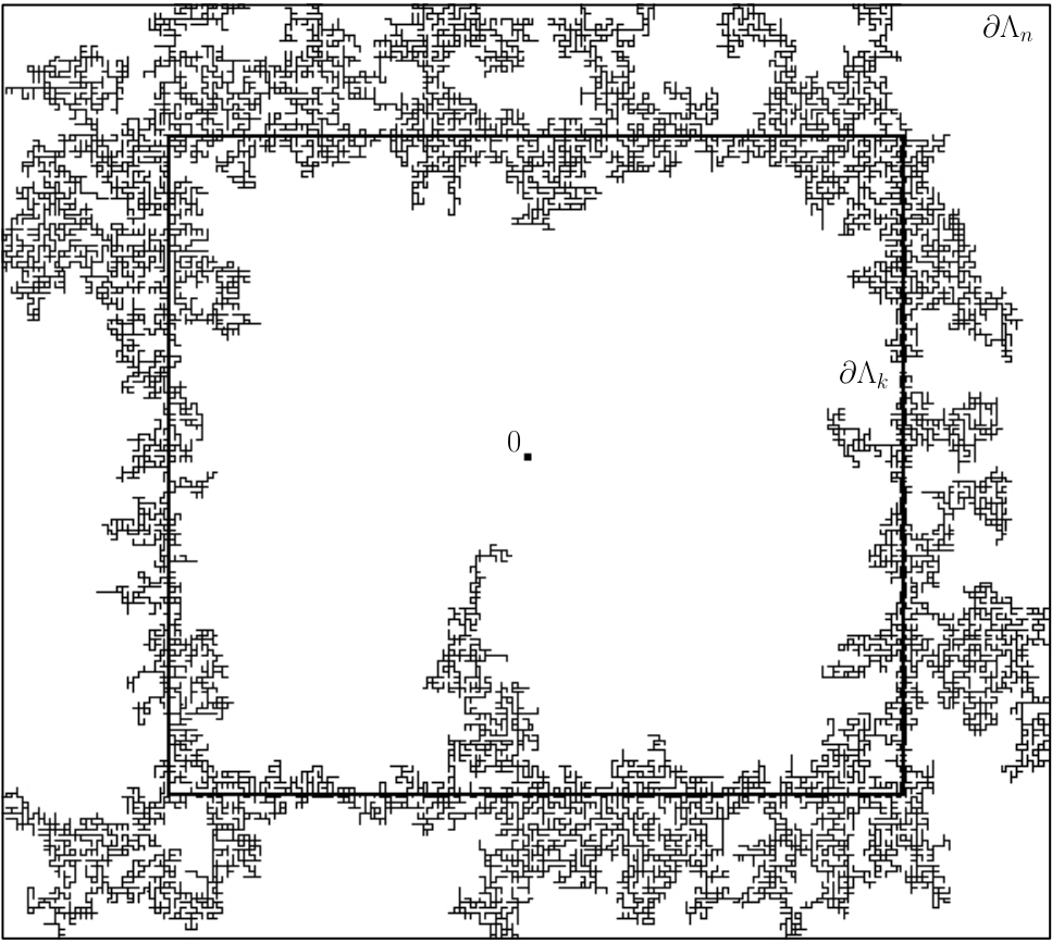
One may simply choose the trivial algorithm checking every edge of the box . Unfortunately, the revealment of the algorithm being 1 for every edge, the OSSS inequality will not bring us interesting information. A slightly better algorithm would be provided by the algorithm discovering the connected component of the origin “from the inside”. Edges far from the origin would then be revealed by the algorithm if (and only if) one of their endpoints is connected to the origin. This provides a good bound for the revealment of edges far from the origin, but edges close to the origin are still revealed with large probability. In order to avoid this last fact, we will rather choose a family of algorithms discovering the connected components of for and observe that the average of their revealment for a fixed edge will always be small.
Proof
For any , we wish to construct an algorithm determining such that for each ,
| (3.5) |
Note that this would conclude the proof since we obtain the target inequality by applying Theorem 2.5 for each and then summing on . As a key, we use that for ,
We describe the algorithm , which corresponds first to an exploration of the connected components in intersecting that does not reveal any edge with both endpoints outside these connected components, and then to a simple exploration of the remaining edges.
More formally, we define (instead of the collection of decision rules ) using two growing sequences and (recall that is the set of edges between two vertices within distance of the origin) that should be understood as follows: at step , represents the set of vertices that the algorithm found to be connected to , and is the set of explored edges discovered by the algorithm until time .
Fix an ordering of the edges in . Set and . Now, assume that and have been constructed and distinguish between two cases:
- •
If there exists an edge with and (if more than one exists, pick the smallest one for the ordering), then set , and set
- •
If does not exist, set to be the smallest (for the ordering) and set and .
As long as we are in the first case, we are still discovering the connected components of . Also, as soon as we are in the second case, we remain in it. The fact that is not greater than the last time we are in the first case gives us (3.5).
Note that may a priori be strictly smaller than the last time we are in the first case (since the algorithm may discover a path of open edges from 0 to or a family of closed edges disconnecting the origin from before discovering the whole connected components of ).
We are now in a position to provide our alternative proof of exponential decay. Fix . Lemma 3.8 together with the Russo-Margulis formula gives
Fix and observe that for , . Then, apply Lemma 3.7 to . Overall, we proved the existence of some such that
- 1.
For , there exists such that for all , .
- 2.
There exists such that for , .
Since was chosen larger than , has no choice but to be equal to , and the proof of Theorem 3.6 therefore follows.
4 Generalizations to monotonic measures
4.1 Random-cluster model
Bernoulli percolation is maybe the most classical example of percolation model, but it is far from being the only one. Percolation models appear in various areas of statistical physics as natural models associated with random walks and spin systems. While Bernoulli percolation is a product measure, and the study of random variables in this context boils down to the study of boolean functions on product spaces, more general percolation models are intrinsically not product measures, and cannot therefore be studied via boolean functions on such spaces.
Recently, the theory of boolean functions has undergone some progress with the study of monotonic measures. As a consequence, certain results valid for product measures extend to this context, enabling us to apply the proofs of the previous sections to more general percolation models. This discovery led to an explosion of results on these percolation models, and we propose to discuss some of the progress here.
Below, we focus on the random-cluster model, which is a percolation model introduced by Fortuin and Kasteleyn in [25] (it is sometimes referred to as the Fortuin-Kasteleyn percolation) as a unification of different models of statistical physics satisfying series/parallel laws when modifying the underlying graph. Let be a finite subgraph of with vertex-set and edge-set . Write and let denote the number of connected components in the graph . The probability measure of the random-cluster model on with edge-weight , connected component-weight and free boundary conditions is defined by
| (4.1) |
for every configuration . The constant is a normalizing constant, referred to as the partition function, defined in such a way that the sum over all configurations equals 1. For , the model can be extended to infinite volume by taking the limit as tends to of the measures . We denote the infinite-volume measure by .
For , the random-cluster model corresponds to Bernoulli percolation. For integers , the model is related to Potts models; see below. For and , the model is connected to electrical networks via Uniform Spanning Trees.
4.2 Computation of the critical point for random-cluster models on
The random-cluster model also undergoes a phase transition at a certain parameter below which the probability that contains an infinite connected component is zero, and above which this probability is 1. For the square lattice, the value of this critical point was predicted in physics over forty years ago. Until recently, only the case of , and very large values of were proved. The following theorem finally answers the conjecture for the whole range of parameters (the condition is not very restrictive, since the behavior of the model is much more tricky for – for instance some averages of increasing boolean functions are not monotonic in ).
Theorem 4.1 (Beffara, DC [3] )
For the random-cluster model on with , the critical point is equal to .
(See also the alternative proofs [15, 16].) Note that for , we recover the previous theorem with equal to . Similarly, we were recently able to prove the following generalization of Theorem 3.6.
Theorem 4.2
Consider the random-cluster model on with .
- 1.
For , there exists such that for all , .
- 2.
There exists such that for , .
The key steps of the proofs of these two theorems are generalizations of Theorems 3.3, 2.2 and 2.5. The generalization of Theorem 3.3 requires the development of a new RSW theory enabled to tackle percolation models with dependency. This theory led to a number of new applications on these models, including a precise description of the critical behavior (see [20, 14, 11] and [12, 13] for reviews). We chose not to discuss this here, and focus on the generalizations of Theorems 2.2 and 2.5.
The random-cluster measure satisfies positive association, a property that enables us to study it using probabilistic techniques. In particular, the measure is monotonic in the following sense. A measure on is monotonic if for any , any , and any satisfying , and ,
As mentioned briefly above, (some of) the theory of boolean functions extends to the case of monotonic measures instead of product measures. In particular, the following two theorems were proved.
Theorem 4.3 (Graham, Grimmett [26])
There exists a constant such that for any monotonic measure on , the following holds. For any increasing boolean function ,
where .
Theorem 4.4 (DC, Raoufi, Tassion [18])
Consider a monotonic measure on . Fix an increasing boolean function and an algorithm . We have
| (4.2) |
where is defined as in the product case.
The proofs of these statements are not immediate. They are combinations of the strategy for product spaces with encoding of monotonic measures via iid random variables. We refer the reader to the corresponding articles [26] and [18] for more details. The dependency of the constants on is fairly explicit. We do not enter into details but let us say that for random-cluster models with away from and , these constants are also away from 0 and infinity.
4.3 Applications to ferromagnetic lattice spin models
We conclude these lectures by mentioning one application of the previous results to the study of random colorings of lattice models. Lattice models have been introduced as discrete models for real life experiments and were later on found useful to model a large variety of phenomena and systems ranging from ferroelectric materials to lattice gas. They also provide discretizations of Euclidean and Quantum Field Theories and are as such important from the point of view of theoretical physics. While the original motivation came from physics, they appeared as extremely complex and rich mathematical objects, whose study required the development of important new tools that found applications in many other domains of mathematics.
The zoo of lattice models is very diverse: it includes models of spin-glasses, quantum chains, random surfaces, spin systems, percolation models. Here, we focus on a smaller class of lattice models called spin systems. These systems are random collections of spin variables assigned to the vertices of a lattice. The archetypal examples of such models are provided by the Ising model, for which spins take values , and the Potts model, for which spins take values in a finite set representing colors (note that the Ising model corresponds to the Potts model with , where and are identified with the two colors 1 and 2). We refer to [28] for more details.
The random-cluster model is related to the Potts models via a simple coupling: one obtains the Potts models by coloring each connected component of the random-cluster configuration uniformly at random66 6 Meaning that for each connected component , one chooses a color uniformly and independently of the choices for other connected components, and then one assigns to every vertex of the color equal to where is the unique connected component of containing . Note that automatically, all the vertices in the same connected component receive the same color.. As a consequence, one can obtain new results on these models, such as rigorous computations of the so-called critical inverse temperatures separating the disordered phase from the ordered phase, the exponential decay of correlations in the disordered phase, the continuity/discontinuity of the phase transition in two dimensions, etc.
There are many models of statistical physics, and therefore many potential applications of dependent percolation models. In particular, let us mention that the techniques described in these notes were also very useful to study continuous percolation models. We refer to [17, 19] for two typical examples. In conclusion, the use of abstract sharp threshold inequalities, which are not necessarily intuitive from the point of view of physics, will probably generalize in the next few years, and we expect a number of breakthroughs in the field based on similar ideas.
References
- [1] M. Aizenman and D. J. Barsky. Sharpness of the phase transition in percolation models. Comm. Math. Phys., 108(3):489–526, 1987.
- [2] W. Beckner. Inequalities in fourier analysis. Ann. of Math, 102(1):159–182, 1975.
- [3] V. Beffara and H. Duminil-Copin. The self-dual point of the two-dimensional random-cluster model is critical for . Probab. Theory Related Fields, 153(3-4):511–542, 2012.
- [4] Béla Bollobás and Oliver Riordan. The critical probability for random Voronoi percolation in the plane is 1/2. Probab. Theory Related Fields, 136(3):417–468, 2006.
- [5] Béla Bollobás and Oliver Riordan. Percolation. Cambridge University Press, New York, 2006.
- [6] Béla Bollobás and Oliver Riordan. A short proof of the Harris-Kesten theorem. Bull. London Math. Soc., 38(3):470–484, 2006.
- [7] Béla Bollobás and Oliver Riordan. Percolation on self-dual polygon configurations. In An irregular mind, volume 21 of Bolyai Soc. Math. Stud., pages 131–217. János Bolyai Math. Soc., Budapest, 2010.
- [8] A. Bonami. Etude des coefficients de fourier des fonctions de lp(g). Ann. Inst. Fourier, 20(2):335–402, 1970.
- [9] Jean Bourgain, Jeff Kahn, Gil Kalai, Yitzhak Katznelson, and Nathan Linial. The influence of variables in product spaces. Israel J. Math., 77(1-2):55–64, 1992.
- [10] S. R. Broadbent and J. M. Hammersley. Percolation processes. I. Crystals and mazes. Proc. Cambridge Philos. Soc., 53:629–641, 1957.
- [11] D. Chelkak, H. Duminil-Copin, C. Hongler, A. Kemppainen, and S. Smirnov. Convergence of Ising interfaces to Schramm’s SLE curves. C. R. Acad. Sci. Paris Math., 352(2):157–161, 2014.
- [12] H. Duminil-Copin. Geometric representations of lattice spin models. book, Edition Spartacus, 2015.
- [13] H. Duminil-Copin. Lectures on the Ising and Potts models on the hypercubic lattice. arXiv:1707.00520, 2017.
- [14] H. Duminil-Copin, M. Gagnebin, M. Harel, I. Manolescu, and V. Tassion. Discontinuity of the phase transition for the planar random-cluster and Potts models with . arXiv preprint arXiv:1611.09877, 2016.
- [15] H. Duminil-Copin and I. Manolescu. The phase transitions of the planar random-cluster and Potts models with are sharp. Probability Theory and Related Fields, 164(3):865–892, 2016.
- [16] H. Duminil-Copin, A. Raoufi, and V. Tassion. A new computation of the critical point for the planar random-cluster model with . arXiv:1604.03702, 2016.
- [17] H. Duminil-Copin, A. Raoufi, and V. Tassion. Exponential decay of connection probabilities for subcritical Voronoi percolation in . arXiv:1705.07978, 2017.
- [18] H. Duminil-Copin, A. Raoufi, and V. Tassion. Sharp phase transition for the random-cluster and potts models via decision trees. arXiv:1705.03104, 2017.
- [19] H. Duminil-Copin, A. Raoufi, and V. Tassion. Subcritical phase of -dimensional Poisson-boolean percolation and its vacant set. arXiv:1805.00695, 2018.
- [20] H. Duminil-Copin, V. Sidoravicius, and V. Tassion. Continuity of the phase transition for planar random-cluster and Potts models with . Communications in Mathematical Physics, 349(1):47–107, 2017.
- [21] H. Duminil-Copin and V. Tassion. A new proof of the sharpness of the phase transition for Bernoulli percolation and the Ising model. Communications in Mathematical Physics, 343(2):725–745, 2016.
- [22] H. Duminil-Copin and V. Tassion. A new proof of the sharpness of the phase transition for Bernoulli percolation on . Enseignement Mathématique, 62(1/2):199–206, 2016.
- [23] P. Erdös and A. Rényi. On random graphs i. Publicationes Mathematicae, 6:290–297, 1959.
- [24] R. Fitzner and R. van der Hofstad. Mean-field behavior for nearest-neighbor percolation in d>10. Electron. J. Probab., 22(43) 65 pp, 2017.
- [25] C. M. Fortuin and P. W. Kasteleyn. On the random-cluster model. I. Introduction and relation to other models. Physica, 57:536–564, 1972.
- [26] B. T. Graham and G. R. Grimmett. Influence and sharp-threshold theorems for monotonic measures. Ann. Probab., 34(5):1726–1745, 2006.
- [27] G. Grimmett. Percolation, volume 321 of Grundlehren der Mathematischen Wissenschaften [Fundamental Principles of Mathematical Sciences]. Springer-Verlag, Berlin, second edition, 1999.
- [28] G. Grimmett. The random-cluster model, volume 333 of Grundlehren der Mathematischen Wissenschaften [Fundamental Principles of Mathematical Sciences]. Springer-Verlag, Berlin, 2006.
- [29] G. Grimmett, S. Janson, and J. Norris. Influence in Product Spaces: BKKKL re-revisited. Influence in product spaces, Probability, Analysis and Number Theory, Advances in Applied Probability 48A:145–152, 2016.
- [30] G. R. Grimmett. Inequalities and entanglements for percolation and random-cluster models. In Perplexing problems in probability, volume 44 of Progr. Probab., pages 91–105. Birkhäuser Boston, Boston, MA, 1999.
- [31] J. Kahn, G. Kalai, and N. Linial. The influence of variables on boolean functions. In 29th Annual Symposium on Foundations of Computer Science, pages 68–80, 1988.
- [32] H. Kesten. The critical probability of bond percolation on the square lattice equals . Comm. Math. Phys., 74(1):41–59, 1980.
- [33] Grigorii A. Margulis. Probabilistic characteristics of graphs with large connectivity. Problemy Peredaci Informacii, 10(2):101–108, 1974.
- [34] M. V. Menshikov. Coincidence of critical points in percolation problems. Dokl. Akad. Nauk SSSR, 288(6):1308–1311, 1986.
- [35] R. O’Donnell, M. Saks, O. Schramm, and R. Servedio. Every decision tree has an influential variable. FOCS, 2005.
- [36] L. Russo. On the critical percolation probabilities. Z. Wahrsch. Verw. Gebiete, 56(2): 229–237, 1981.
- [37] L. Russo. An approximate zero-one law. Z. Wahrsch. Verw. Gebiete, 61(1):129–139, 1982.
- [38] P. D. Seymour and D. J. A. Welsh. Percolation probabilities on the square lattice. Ann. Discrete Math., 3:227–245, 1978. Advances in graph theory (Cambridge Combinatorial Conf., Trinity College, Cambridge, 1977).
- [39] M. Talagrand. On Russo’s approximate zero-one law. Ann. Probab., 22(3):1576–1587, 1994.
- [40] Vincent Tassion. Planarité et localité en percolation. PhD thesis, ENS Lyon, 2014.
- [41] Vincent Tassion. Crossing probabilities for voronoi percolation. Annals of Probability, 44(5):3385–3398, 2016. arXiv:1410.6773.
- [42] A. C. Yao. Probabilistic computations: Toward a unified measure of complexity. In Foundations of Computer Science, 1977., 18th Annual Symposium on, pages 222–227. IEEE, 1977.