Causal isotonic regression
Abstract
In observational studies, potential confounders may distort the causal relationship between an exposure and an outcome. However, under some conditions, a causal dose-response curve can be recovered using the -computation formula. Most classical methods for estimating such curves when the exposure is continuous rely on restrictive parametric assumptions, which carry significant risk of model misspecification. Nonparametric estimation in this context is challenging because in a nonparametric model these curves cannot be estimated at regular rates. Many available nonparametric estimators are sensitive to the selection of certain tuning parameters, and performing valid inference with such estimators can be difficult. In this work, we propose a nonparametric estimator of a causal dose-response curve known to be monotone. We show that our proposed estimation procedure generalizes the classical least-squares isotonic regression estimator of a monotone regression function. Specifically, it does not involve tuning parameters, and is invariant to strictly monotone transformations of the exposure variable. We describe theoretical properties of our proposed estimator, including its irregular limit distribution and the potential for doubly-robust inference. Furthermore, we illustrate its performance via numerical studies, and use it to assess the relationship between BMI and immune response in HIV vaccine trials.
1 Introduction
1.1 Motivation and literature review
Questions regarding the causal effect of an exposure on an outcome are ubiquitous in science. If investigators are able to carry out an experimental study in which they randomly assign a level of exposure to each participant and then measure the outcome of interest, estimating a causal effect is generally straightforward. However, such studies are often not feasible, and data from observational studies must be relied upon instead. Assessing causality is then more difficult, in large part because of potential confounding of the relationship between exposure and outcome. Many nonparametric methods have been proposed for drawing inference about a causal effect using observational data when the exposure of interest is either binary or categorical – these include, among others, inverse probability weighted (IPW) estimators (Horvitz and Thompson, 1952), augmented IPW estimators (Scharfstein et al., 1999; Bang and Robins, 2005), and targeted minimum loss-based estimators (TMLE) (van der Laan and Rose, 2011).
In practice, many exposures are continuous, in the sense that they may take any value in an interval. A common approach to dealing with such exposures is to simply discretize the interval into two or more regions, thus returning to the categorical exposure setting. However, it is frequently of scientific interest to learn the causal dose-response curve, which describes the causal relationship between the exposure and outcome across a continuum of the exposure. Much less attention has been paid to continuous exposures. Robins (2000) and Zhang et al. (2016) studied this problem using parametric models, and Neugebauer and van der Laan (2007) considered inference on parameters obtained by projecting a causal dose-response curve onto a parametric working model. Other authors have taken a nonparametric approach instead. Rubin and van der Laan (2006) and Díaz and van der Laan (2011) discussed nonparametric estimation using flexible data-adaptive algorithms. Kennedy et al. (2017) proposed an estimator based on local linear smoothing. Finally, van der Laan et al. (2018) recently presented a general framework for inference on parameters that fail to be smooth enough as a function of the data-generating distribution and for which regular root- estimation theory is therefore not available. This is indeed the case for the causal dose-response curve, and van der Laan et al. (2018) discussed inference on such a parameter as a particular example.
Despite a growing body of literature on nonparametric estimation of causal dose-response curves, to the best of our knowledge, existing methods do not permit valid large-sample inference and may be sensitive to the selection of certain tuning parameters. For instance, smoothing-based methods are often sensitive to the choice of a kernel function and bandwidth, and these estimators typically possess non-negligible asymptotic bias, which complicates the task of performing valid inference.
In many settings, it may be known that the causal dose-response curve is monotone in the exposure. For instance, exposures such as daily exercise performed, cigarettes smoked per week, and air pollutant levels are all known to have monotone relationships with various health outcomes. In such cases, an extensive literature suggests that monotonicity may be leveraged to derive estimators with desirable properties – the monograph of Groeneboom and Jongbloed (2014) provides a comprehensive overview. For example, in the absence of confounding, isotonic regression may be employed to estimate the causal dose-response curve (Barlow et al., 1972). The isotonic regression estimator does not require selection of a kernel function or bandwidth, is invariant to strictly increasing transformations of the exposure, and upon centering and scaling by , converges in law pointwise to a symmetric limit distribution with mean zero (Brunk, 1970). The latter property is useful since it facilitates asymptotically valid pointwise inference.
Nonparametric inference on a monotone dose-response curve when the exposure-outcome relationship is confounded is more difficult to tackle and is the focus of this manuscript. To the best of our knowledge, this problem has not been comprehensively studied before.
1.2 Parameter of interest and its causal interpretation
The prototypical data unit we consider is , where is a response, a continuous exposure, and a vector of covariates. The support of the true data-generating distribution is denoted by , where , is an interval, and . Throughout, the use of subscript refers to evaluation at or under . For example, we write and to denote and , respectively, and to denote expectation under .
Our parameter of interest is the so-called -computed regression function from to , defined as
where the outer expectation is with respect to the marginal distribution of . In some scientific contexts, may have a causal interpretation. Adopting the Neyman-Rubin potential outcomes framework, for each , we denote by a unit’s potential outcome under exposure level . The causal parameter corresponds to the average outcome under assignment of the entire population to exposure level . The resulting curve is what we formally define as the causal dose-response curve. Under varying sets of causal conditions, may be identified with functionals of the observed data distribution, such as the unadjusted regression function or the -computed regression function .
Suppose that (i) each unit’s potential outcomes are independent of all other units’ exposures; and (ii) the observed outcome equals the potential outcome corresponding to the exposure level actually received. Identification of further depends on the relationship between and . If (i) and (ii) hold, and in addition, (iii) and are independent, and (iv) the marginal density of is positive at , then . Condition (iii) typically only holds in experimental studies (e.g., randomized trials). In observational studies, there are often common causes of and – so-called confounders of the exposure-outcome relationship – that induce dependence. In such cases, and do not generally coincide. However, if contains a sufficiently rich collection of confounders, it may still be possible to identify from the observed data. If (i) and (ii) hold, and in addition, (v) and are conditionally independent given , and (vi) the conditional density of given is almost surely positive at , then . This is a fundamental result in causal inference (Robins, 1986; Gill and Robins, 2001). Whenever , our methods can be interpreted as drawing inference on the causal dose-response parameter .
We note that the definition of the counterfactual outcome presupposes that the intervention setting is uniquely defined. In many situations, this stipulation requires careful thought. For example, in Section 6 we consider an application in which body mass index (BMI) is the exposure of interest. There is an ongoing scientific debate about whether such an exposure leads to a meaningful causal interpretation, since it is not clear what it means to intervene on BMI.
Even if the identifiability conditions stipulated above do not strictly hold or the scientific question is not causal in nature, when is associated with both and , often has a more appealing interpretation than the unadjusted regression function . Specifically, may be interpreted as the average value of in a population with exposure fixed at but otherwise characteristic of the study population with respect to . Because involves both adjustment for and marginalization with respect to a single reference population that does not depend on the value , the comparison of over different values of is generally more meaningful than for .
When , the parameter is not pathwise differentiable at with respect to the nonparametric model (Díaz and van der Laan, 2011). Heuristically, due to the continuous nature of , corresponds to a local feature of . As a result, regular root- rate estimators cannot be expected, and standard methods for constructing efficient estimators of pathwise differentiable parameters in nonparametric and semiparametric models (e.g., estimating equations, one-step estimation, targeted minimum loss-based estimation) cannot be used directly to target and obtain inference on .
1.3 Contribution and organization of the article
We denote by the distribution function of under , by the class of non-decreasing real-valued functions on , and by the class of strictly increasing and continuous distribution functions supported on . The statistical model we will work in is , which consists of the collection of distributions for which is non-decreasing over and the marginal distribution of is continuous with positive Lebesgue density over .
In this article, we study nonparametric estimation and inference on the -computed regression function for use when is a continuous exposure and is known to be monotone. Specifically, our goal is to make inference about for using independent observations drawn from . This problem is an extension of classical isotonic regression to the setting in which the exposure-outcome relationship is confounded by recorded covariates – this is why we refer to the method proposed as causal isotonic regression. As mentioned above, to the best of our knowledge, nonparametric estimation and inference on a monotone -computed regression function has not been comprehensively studied before. In what follows, we:
- 1.
show that our proposed estimator generalizes the unadjusted isotonic regression estimator to the more realistic scenario in which there is confounding by recorded covariates;
- 2.
investigate finite-sample and asymptotic properties of the proposed estimator, including invariance to strictly increasing transformations of the exposure, doubly-robust consistency, and doubly-robust convergence in distribution to a non-degenerate limit;
- 3.
derive practical methods for constructing pointwise confidence intervals, including intervals that have valid doubly-robust calibration;
- 4.
illustrate numerically the practical performance of the proposed estimator.
We note that in Westling and Carone (2019), we studied estimation of as one of several examples of a general approach to monotonicity-constrained inference. Here, we provide a comprehensive examination of estimation of a monotone dose-response curve. In particular, we establish novel theory and methods that have important practical implications. First, we provide conditions under which the estimator converges in distribution even when one of the nuisance estimators involved in the problem is inconsistent. This contrasts with the results in Westling and Carone (2019), which required that both nuisance parameters be estimated consistently. We also propose two estimators of the scale parameter arising in the limit distribution, one of which requires both nuisance estimators to be consistent, and the other of which does not. Second, we demonstrate that our estimator is invariant to strictly monotone transformations of the exposure. Third, we study the joint convergence of our proposed estimator at two points, and use this result to construct confidence intervals for causal effects. Fourth, we study the behavior of our estimator in the context of discrete exposures. Fifth, we propose an alternative estimator based on cross-fitting of the nuisance estimators, and demonstrate that this strategy removes the need for empirical process conditions required in Westling and Carone (2019). Finally, we investigate the behavior of our estimator in comprehensive numerical studies, and compare its behavior to that of the local linear estimator of Kennedy et al. (2017).
The remainder of the article is organized as follows. In Section 2, we concretely define the proposed estimator. In Section 3, we study theoretical properties of the proposed estimator. In Section 4, we propose methods for pointwise inference. In Section 5, we perform numerical studies to assess the performance of the proposed estimator, and in Section 6, we use this procedure to investigate the relationship between BMI and immune response to HIV vaccines using data from several randomized trials. Finally, we provide concluding remarks in Section 7. Proofs of all theorems are provided in Supplementary Material.
2 Proposed approach
2.1 Review of isotonic regression
Since the proposed estimator of builds upon isotonic regression, we briefly review the classical least-squares isotonic regression estimator of . The isotonic regression of on is the minimizer in of over all monotone non-decreasing functions. This minimizer can be obtained via the Pool Adjacent Violators Algorithm (Ayer et al., 1955; Barlow et al., 1972), and can also be represented in terms of greatest convex minorants (GCMs). The GCM of a bounded function on an interval is defined as the supremum over all convex functions such that . Letting be the empirical distribution function of , can be shown to equal the left derivative, evaluated at , of the GCM over the interval of the linear interpolation of the so-called cusum diagram
where and is the value of corresponding to the observation with smallest value of .
The isotonic regression estimator has many attractive properties. First, unlike smoothing-based estimators, isotonic regression does not require the choice of a kernel function, bandwidth, or any other tuning parameter. Second, it is invariant to strictly increasing transformations of . Specifically, if is a strictly increasing function, and is the isotonic regression of on , it follows that . Third, is uniformly consistent on any strict subinterval of . Fourth, converges in distribution to for any interior point of at which , and exist, and are positive and continuous in a neighborhood of . Here, , where denotes a two-sided Brownian motion originating from zero, and is said to follow Chernoff’s distribution. Chernoff’s distribution has been extensively studied: among other properties, it is a log-concave and symmetric law centered at zero, has moments of all orders, and can be approximated by a distribution (Chernoff, 1964; Groeneboom and Wellner, 2001). It appears often in the limit distribution of monotonicity-constrained estimators.
2.2 Definition of proposed estimator
For any given , we define the outcome regression pointwise as , and the normalized exposure density as , where is the evaluation at of the conditional density function of given and is the marginal density function of under . Additionally, we define the pseudo-outcome as
As noted by Kennedy et al. (2017), if either or . They used this fact to motivate an estimator of , defined as the local linear regression with bandwidth of the pseudo-outcomes on , where is an estimator of , is an estimator of , and is the empirical distribution function based on . The study of this nonparametric regression problem is not standard because these pseudo-outcomes are dependent when the nuisance function estimators and are estimated from the data. Nevertheless, Kennedy et al. (2017) showed that their estimator is consistent if either or is consistent. Additionally, under regularity conditions, they showed that if both nuisance estimators converge fast enough and the bandwidth tends to zero at rate , then , where is an asymptotic bias depending on the second derivative of , and is an asymptotic variance.
In our setting, is known to be monotone. Therefore, instead of using a local linear regression to estimate the conditional mean of the pseudo-outcomes, it is natural to consider as an estimator the isotonic regression of the pseudo-outcomes on . Using the GCM representation of isotonic regression stated in the previous section, we can summarize our estimation procedure as follows:
- 1.
Construct estimators and of and , respectively.
- 2.
For each in the unique values of , compute and set
(1) - 3.
Compute the GCM of the set of points over .
- 4.
Define as the left derivative of evaluated at .
As in the work of Kennedy et al. (2017), while the proposed estimator can be defined as an isotonic regression, the asymptotic properties of our estimator do not appear to simply follow from classical results for isotonic regression because the pseudo-outcomes depend on the estimators , and , which themselves depend on all the observations. However, is of generalized Grenander-type, and thus the asymptotic results of Westling and Carone (2019) can be used to study its asymptotic properties. To see that is a generalized Grenander-type estimator, we define and note that since and are increasing, so is . Therefore, the primitive function is convex. Next, we define , so that . The parameter is pathwise differentiable at in for each , and its nonparametric efficient influence function can be computed to be
Denoting by any estimator of compatible with estimators , , and of , , and , respectively, the one-step estimator of is given by , where we define . This one-step estimator is equivalent to that defined in (1). We then define for the empirical quantile function of as our estimator of , and as the left derivative of the GCM of . Thus, we find that is the estimator defined in steps 1–4. This form of the estimator was described in Westling and Carone (2019), where it was briefly discussed as one of several examples of a general strategy for nonparametric monotone inference.
If were only known to be monotone on a fixed sub-interval , we would define as the marginal distribution function restricted to , and as its empirical counterpart. Similarly, in (1) would be replaced with . In all other respects, our estimation procedure would remain the same.
Finally, as alluded to earlier, we observe that the proposed estimator generalizes classical isotonic regression in a way we now make precise. If it is known that is independent of (Condition 1), so that for all supported , we may take . If, furthermore, it is known that is independent of given (Condition 2), then we may construct such that for all supported . Inserting and any such into (1), we obtain that and thus that for each . Hence, in this case, our estimator reduces to least-squares isotonic regression.
3 Theoretical properties
3.1 Invariance to strictly increasing exposure transformations
An important feature of the proposed estimator is that, as with the isotonic regression estimator, it is invariant to any strictly increasing transformation of . This is a desirable property because the scale of a continuous exposure is often arbitrary from a statistical perspective. For instance, if is temperature, whether is measured in degrees Fahrenheit, Celsius or Kelvin does not change the information available. In particular, if the parameters and correspond to using as exposure and , respectively, for some strictly increasing transformation, then and encode exactly the same information about the effect of on after adjusting for . It is therefore natural to expect any sensible estimator to be invariant to the scale on which the exposure is measured.
Setting for a strictly increasing function , we first note that the function is non-decreasing. Next, we define and , where is the evaluation at of the conditional density function of given and is the marginal density function of under , and we denote by and estimators of and , respectively. The estimation procedure defined in the previous section but using exposure instead of then leads to estimator , where is the empirical distribution function based on , and is the left derivative of the GCM of for
If it is the case that and , implying that nuisance estimators and are themselves invariant to strictly increasing transformation of , then we have that , and so, . It follows then that . In other words, the proposed estimator of is invariant to any strictly increasing transformation of the exposure variable.
We note that it is easy to ensure that and . Set , which is also equal to , and let be an estimator of the conditional mean of given . Then, taking , we have that satisfies the desired property. Similarly, letting be an estimator of the conditional density of given , and setting , we may take .
3.2 Consistency
We now provide sufficient conditions under which consistency of is guaranteed. Our conditions require controlling the uniform entropy of certain classes of functions. For a uniformly bounded class of functions , a finite discrete probability measure , and any , the -covering number of relative to the metric is the smallest number of -balls of radius less than or equal to needed to cover . The uniform -entropy of is then defined as , where the supremum is taken over all finite discrete probability measures. For a thorough treatment of covering numbers and their role in empirical process theory, we refer readers to van der Vaart and Wellner (1996).
Below, we state three sufficient conditions we will refer to in the following theorem.
- (A1)
-
There exist constants and such that, almost surely as , and are contained in classes of functions and , respectively, satisfying:
- 1.
for all , and for all ;
- 2.
and for all .
- 1.
- (A2)
-
There exist and such that and .
- (A3)
-
There exist subsets and of such that and:
- 1.
for all ;
- 2.
for all ;
- 3.
and for all .
- 1.
Under these three conditions, we have the following result.
Theorem 1 (Consistency).
If conditions (A1)–(A3) hold, then for any value such that , is continuous at , and is strictly increasing in a neighborhood of . If is uniformly continuous and is strictly increasing on , then for any bounded strict subinterval .
We note that in the pointwise statement of Theorem 1, is required to be in the interior of , and similarly, the uniform statement of Theorem 1 only covers strict subintervals of . This is due to the well-known boundary issues with Grenander-type estimators. Various remedies have been proposed in particular settings, and it would be interesting to consider these in future work (see, e.g., Woodroofe and Sun, 1993; Balabdaoui et al., 2011; Kulikov and Lopuhaä, 2006).
Condition (A1) requires that and eventually be contained in uniformly bounded function classes that are small enough for certain empirical process terms to be controlled. This condition is easily satisfied if, for instance, and are parametric classes. It is also satisfied for many infinite-dimensional function classes. Uniform entropy bounds for many such classes may be found in Chapter 2.6 of van der Vaart and Wellner (1996). We note that there is an asymmetry between the entropy requirements for and in part (b) of (A1). This is due to the term appearing in . To control this term, we use an upper bound of the form from the theory of empirical -processes (Nolan and Pollard, 1987) – this contrasts with the uniform entropy integral that bounds ordinary empirical processes indexed by a uniformly bounded class . In Section 3.7, we consider the use of cross-fitting to avoid the entropy conditions in (A1).
Condition (A2) requires that and tend to limit functions and , and condition (A3) requires that either or for -almost every . If either (i) and are null sets or (ii) and are null sets, then condition (A3) is known simply as double-robustness of the estimator relative to the nuisance functions and : is consistent as long as or . Doubly-robust estimators are at this point a mainstay of causal inference and have been studied for over two decades (see, e.g., Robins et al., 1994; Rotnitzky et al., 1998; Scharfstein et al., 1999; van der Laan and Robins, 2003; Neugebauer and van der Laan, 2005; Bang and Robins, 2005). However, (A3) is more general than classical double-robustness, as it allows neither nor to tend to their true counterparts over the whole domain, as long as at least one of or tends to the truth for almost every point in the domain.
3.3 Convergence in distribution
We now study the convergence in distribution of for fixed . We first define for any square-integrable functions , and the pseudo-distance
| (2) |
We also denote by the conditional variance of given and under . Below, we will refer to these two additional conditions:
- (A4)
-
There exists such that:
- 1.
;
- 2.
;
- 3.
.
- 1.
- (A5)
-
and are continuously differentiable in a neighborhood of uniformly over .
Under conditions introduced so far, we have the following distributional result.
Theorem 2 (Convergence in distribution).
If conditions (A1)–(A5) hold, then
for any such that , where follows the standard Chernoff distribution and
with denoting .
We note that the limit distribution in Theorem 2 is the same as that of the standard isotonic regression estimator up to a scale factor. As noted above, when either (i) and are independent given or (ii) is independent of , the functions and coincide. As such, we can directly compare the respective limit distributions of and under these conditions. When both and , is asymptotically more concentrated than in scenario (i), and less concentrated in scenario (ii). This is analogous to findings in linear regression, where including a covariate uncorrelated with the outcome inflates the standard error of the estimator of the coefficient corresponding to the exposure, while including a covariate correlated with the outcome but uncorrelated with the exposure deflates its standard error.
Condition (A4) requires that, on the set where is consistent but is not, converges faster than uniformly in a neighborhood of , and similarly for on the set . On the set where both and are consistent, only the product of their rates of convergence must be faster than . Hence, a non-degenerate limit theory is available as long as at least one of the nuisance estimators is consistent at a rate faster than , even if the other nuisance estimator is inconsistent. This suggests the possibility of performing doubly-robust inference for , that is, of constructing confidence intervals and tests based on with valid calibration even when one of and is inconsistently estimated. This is explored in Section 4. Finally, as in Theorem 1, we allow that neither nor be consistent everywhere, as long as for -almost every at least one of or is consistent.
We remark that if it is known that is consistent for in an sense at rate faster than , the isotonic regression of the plug-in estimator – which can be equivalently obtained by setting in the construction of – achieves a faster rate of convergence to than does . This might motivate an analyst to use rather than in such a scenario. However, the consistency of hinges entirely on the fact that , and in particular, will be inconsistent if , even if . Additionally, the estimator may not generally admit a tractable limit theory upon which to base the construction of valid confidence intervals, particularly when machine learning methods are used to build .
3.4 Grenander-type estimation without domain transformation
As indicated earlier, the isotonic regression estimator based on estimated pseudo-outcomes coincides with a generalized Grenander-type estimator for which the marginal exposure empirical distribution function is used as domain transformation. An alternative estimator could be constructed via Grenander-type estimation without the use of any domain transformation. Specifically, we let be fixed, and we define . Under regularity conditions, for , the one-step estimator of given by
is asymptotically efficient, where is an estimator of , the conditional density of given under . The left derivative of the GCM of over defines an alternative estimator .
It is natural to ask how compares to the estimator we have studied thus far. First, we note that, unlike , neither generalizes the classical isotonic regression estimator nor is invariant to strictly increasing transformations of . Additionally, utilizing the transformation fixes as the interval over which the GCM should be performed. If is known to be a bounded set, can be taken as the endpoints of , but otherwise the domain must be chosen in defining . Turning to an asymptotic analysis, using the results of Westling and Carone (2019), it is possible to establish conditions akin to (A1)–(A5) under which with scale parameter
where is the limit of in probability. We denote by and the limit scaling factors of and , respectively. If and , then , and and have the same limit distribution. If instead but , this is no longer the case. In fact, we can show that
Hence, when the outcome regression estimator is inconsistent, gains in efficiency are achieved by utilizing the transformation, and the relative gain in efficiency is directly related to the amount of asymptotic bias in the estimation of .
3.5 Discrete domains
In some circumstances, the exposure is discrete rather than continuous. Our estimator works equally well in these cases, since, as we highlight below, it turns out to then be asymptotically equivalent to the well-studied augmented IPW (AIPW) estimator. As a result, the large-sample properties of our estimator can be derived from the large-sample properties of the AIPW estimator, and asymptotically valid inference can be obtained using standard influence function-based techniques.
Suppose that and for all and . Our estimation procedure remains the same with one exception: in defining , we now take to be the conditional probability rather than the corresponding conditional density, and we take as the marginal probability rather than the corresponding marginal density. We then set as the estimator of , where is any estimator of and for . In all other respects, our estimation procedure is identical to that defined previously. With these definitions, we denote by the estimated pseudo-outcome for observation . Our estimator is then the isotonic regression of on . However, since for each there is a unique such that , this is equivalent to performing isotonic regression of on , where . It is straightforward to see that
which is exactly the AIPW estimator of . Therefore, in this case, our estimator reduces to the isotonic regression of the classical AIPW estimator constructed separately for each element of the exposure domain.
The large-sample properties of , including doubly-robust consistency and convergence in distribution at the regular parametric rate , are well-established (Robins et al., 1994). Therefore, many properties of in this case can be determined using the results of Westling et al. (2018), which studied the behavior of the isotonic correction of an initial estimator. In particular, as long as is non-decreasing on . Uniform consistency of over thus implies uniform consistency of . Furthermore, if is strictly increasing on and converges in distribution, then , so that large-sample standard errors for are also valid for . If is not strictly increasing on but instead has flat regions, then is more efficient than on these regions, and confidence intervals centered around but based upon the limit theory for will be conservative.
3.6 Large-sample results for causal effects
In many applications, in addition to the causal dose response curve itself, causal effects of the form are of scientific interest as well. Under the identification conditions discussed in Section 1.2 applied to each of and , such causal effects are identified with the observed-data parameter . A natural estimator for such a causal effect in our setting is . If the conditions of Theorem 1 hold for both and , then the continuous mapping theorem implies that . However, since Theorem 2 only provides marginal distributional results, and thus does not describe the joint convergence of , it cannot be used to determine the large-sample behavior of . The following result demonstrates that such joint convergence can be expected under the aforementioned conditions, and that the bivariate limit distribution of has independent components.
Theorem 3 (Joint convergence in distribution).
If conditions (A1)–(A5) hold for and , then converges in distribution to , where and are independent standard Chernoff distributions and the scale parameter is as defined in Theorem 2.
Theorem 3 implies that, under the stated conditions, converges in distribution to .
3.7 Use of cross-fitting to avoid empirical process conditions
Theorems 1 and 2 reveal that the statistical properties of depend on the nuisance estimators and in two important ways. First, we require in condition (A1) that or fall in small enough classes of functions, as measured by metric entropy, in order to control certain empirical process remainder terms. Second, we require in conditions (A2)–(A3) that at least one of or be consistent almost everywhere (for consistency), and in condition (A4) that the product of their rates of convergence be faster than (for convergence in distribution). In observational studies, researchers can rarely specify a priori correct parametric models for and . This motivates use of data-adaptive estimators of these nuisance functions in order to meet the second requirement. However, such estimators often lead to violations of the first requirement, or it may be onerous to determine that they do not. Thus, because it may be difficult to find nuisance estimators that are both data-adaptive enough to meet required rates of convergence and fall in small enough function classes to make empirical process terms negligible, simultaneously satisfying these two requirements can be challenging in practice.
In the context of asymptotically linear estimators, it has been noted that cross-fitting nuisance estimators can resolve this challenge by eliminating empirical process conditions (Zheng and van der Laan, 2011; Belloni et al., 2018; Kennedy, 2019). We therefore propose employing cross-fitting of and in the estimation of in order to avoid entropy conditions in Theorems 1 and 2. Specifically, we fix and suppose that the indices are randomly partitioned into sets . We assume for convenience that is an integer and that for each , but all of our results hold as long as . For each , we define as the training set for fold , and denote by and the nuisance estimators constructed using only the observations from . We then define pointwise the cross-fitted estimator of as
| (3) |
Finally, the cross-fitted estimator of is constructed using steps 1–4 outlined in Section 2.2, with replaced by .
As we now demonstrate, utilizing the cross-fitted estimator allows us to avoid the empirical process condition (A1b). We first introduce the following two conditions, which are analogues of conditions (A1) and (A2).
- (B1)
-
There exist constants such that, almost surely as and for all , and are contained in classes of functions and , respectively, satisfying:
- 1.
for all , and for all ;
and for almost all .
- 1.
- (B2)
-
There exist and such that and .
We then have the following analogue of Theorem 1 establishing consistency of the cross-fitted estimator .
Theorem 4 (Consistency of the cross-fitted estimator).
If conditions (B1)–(B2) and (A3) hold, then for any such that , is continuous at , and is strictly increasing in a neighborhood of . If is uniformly continuous and is strictly increasing on , then for any bounded strict subinterval .
For convergence in distribution, we introduce the following analogue of condition (A4).
- (B4)
-
There exists such that:
- 1.
;
- 2.
;
- 3.
.
- 1.
We then have the following analogue of Theorem 2 for the cross-fitted estimator .
Theorem 5 (Convergence in distribution for the cross-fitted estimator).
If conditions (B1), (B2), (A3), (B4), and (A5) hold, then for any such that .
The conditions of Theorems 4 and 5 are analogous to those of Theorems 1 and 2, with the important exception that the entropy condition (A1b) is no longer required. Therefore, the estimators and may be as data-adaptive as one desires without concern for empirical process terms, as long as they satisfy the boundedness conditions stated in (B1).
4 Construction of confidence intervals
4.1 Wald-type confidence intervals
The distributional results of Theorem 2 can be used to construct a confidence interval for . Since the limit distribution of is symmetric around zero, a Wald-type construction seems appropriate. Specifically, writing and denoting by any consistent estimator of , a Wald-type level asymptotic confidence interval for is given by
where denotes the quantile of . Quantiles of the standard Chernoff distribution have been numerically computed and tabulated on a fine grid (Groeneboom and Wellner, 2001), and are readily available in the statistical programming language R. Estimation of involves, either directly or indirectly, estimation of and . We focus first on the former.
We note that with . This suggests that we could either estimate and separately and consider the ratio of these estimators, or that we could instead estimate directly and compose it with the estimator of already available. The latter approach has the desirable property that the resulting scale estimator is invariant to strictly monotone transformations of the exposure. As such, this is the strategy we favor. To estimate , we recall that the estimator from Section 2 is a step function and is therefore not differentiable. A natural solution consists of computing the derivative of a smoothed version of . We have found local quadratic kernel smoothing of points , for the midpoints of the jump points of , to work well in practice.
Theorem 3 can be used to construct Wald-type confidence intervals for causal effects of the form . We first construct estimates and of the scale parameters and , respectively, and then compute an approximation of the -quantile of , where and are independent Chernoff distributions, using Monte Carlo simulations, for example. An asymptotic level Wald-type confidence interval for is then .
In the next two subsections, we discuss different strategies for estimating the scale factor .
4.2 Scale estimation relying on consistent nuisance estimation
We first consider settings in which both and are consistent estimators, that is, and . In such cases, we have that with denoting the conditional variance . Any regression technique could be used to estimate the conditional expectation of given and , yielding an estimator of . A plug-in estimator of is then given by
Provided , and are consistent estimators of , and , respectively, is a consistent estimator of . We note that in the special case of a binary outcome, the fact that motivates the use of as estimator , and thus eliminates the need for further regression beyond the construction of and . In practice, we typically recommend the use of an ensemble method – for example, the SuperLearner (van der Laan et al., 2007) – to combine a variety of regression techniques, including machine learning techniques, to minimize the risk of inconsistency of , and .
4.3 Doubly-robust scale estimation
As noted above, Theorem 2 provides the limit distribution of even if one of the nuisance estimators is inconsistent, as long as the consistent nuisance estimator converges fast enough. We now show how we may capitalize on this result to provide a doubly-robust estimator of . Since is itself a doubly-robust estimator of , so will be the proposed estimator of and hence also of the resulting estimator of . This contrasts with the estimator of described in the previous section, which required the consistency of both and .
To construct an estimator of consistent even if either or , we begin by noting that , where for some bounded density function with bounded support, and we have defined
Setting with the empirical distribution based on , we define with obtained by substituting , , and by , , and , respectively, in the definition of . Under conditions (A1)–(A5), it can be shown that by standard kernel smoothing arguments for any sequence . In particular, is consistent under the general form of doubly-robustness specified by condition (A3).
To determine an appropriate value of the bandwidth in practice, we propose the following empirical criterion. We first define the integrated scale , and construct the estimator for any candidate . Furthermore, we observe that , which suggests the use of the empirical estimator . This motivates us to define , that is, the value of that makes and closest. The proposed doubly-robust estimator of is thus .
We make two final remarks regarding this doubly-robust estimator of . First, we note that this estimator only depends on and through the ranks and . Hence, as before, our estimator is invariant to strictly monotone transformations of the exposure . Second, we note that if does not depend on and , tends to the conditional variance , which is precisely the scale parameter appearing in standard isotonic regression.
4.4 Confidence intervals via sample splitting
As an alternative, we note here that the sample-splitting method recently proposed by Banerjee et al. (2019) could also be used to perform inference. Specifically, to implement their approach in our context, we randomly split the sample into subsets of roughly equal size, perform our estimation procedure on each subset to form subset-specific estimates , and then define . Banerjee et al. (2019) demonstrated that if is fixed, then under mild conditions has strictly better asymptotic mean squared error than , and that for moderate ,
| (4) |
forms an asymptotic level confidence interval for , where and is the -quantile of the -distribution with degrees of freedom.
5 Numerical studies
In this section, we perform numerical experiments to assess the performance of the proposed estimators of and of the three approaches for constructing confidence intervals, which we also compare to that of the local linear estimator and associated confidence intervals proposed in Kennedy et al. (2017).
In our experiments, we simulate data as follows. First, we generate as a vector of four independent standard normal variates. A natural next step would be to generate given . However, since our estimation procedures requires estimating the conditional density of given , we instead generate given , and then transform to obtain . This strategy makes it easier to construct correctly-specified parametric nuisance estimators in the context of these simulations. Given , we generate from the distribution with conditional density function for . We note that for all and , and also, that , so that is marginally uniform. We then take to be the evaluation at of the quantile function of an equal-weight mixture of two normal distributions with means and and standard deviation 1, which implies that is marginally distributed according to this bimodal normal mixture. Finally, conditionally upon and , we simulate as a Bernoulli random variate with conditional mean function given by , where denotes . We set , , and in the experiments we report on.
We estimate the true confounder-adjusted dose-response curve using the causal isotonic regression estimator , the local linear estimator of Kennedy et al. (2017), and the sample-splitting version of proposed by Banerjee et al. (2019) with splits. For the local linear estimator, we use the data-driven bandwidth selection procedure proposed in Section 3.5 of Kennedy et al. (2017). We consider three settings in which either both and are consistent; only consistent; and only consistent. To construct a consistent estimator , we use a correctly specified logistic regression model, whereas to construct a consistent estimator , we use a maximum likelihood estimator based on a correctly specified parametric model. To construct an inconsistent estimator , we still use a logistic regression model but omit covariates , and all interactions. To construct an inconsistent estimator , we posit the same parametric model as before but omit and . We construct pointwise confidence intervals for in each setting using the Wald-type construction described in Section 4 using both the plug-in and doubly-robust estimators of . We expect intervals based on the doubly-robust estimator of to provide asymptotically correct coverage rates for for each of the three settings, but only expect asymptotically correct coverage rates in the first setting when the plug-in estimator of is used. We construct pointwise confidence intervals for the local linear estimator using the procedure proposed in Kennedy et al. (2017), and for the sample splitting procedure using the procedure discussed in Section 4.4. We consider the performance of these inferential procedures for values of between and .
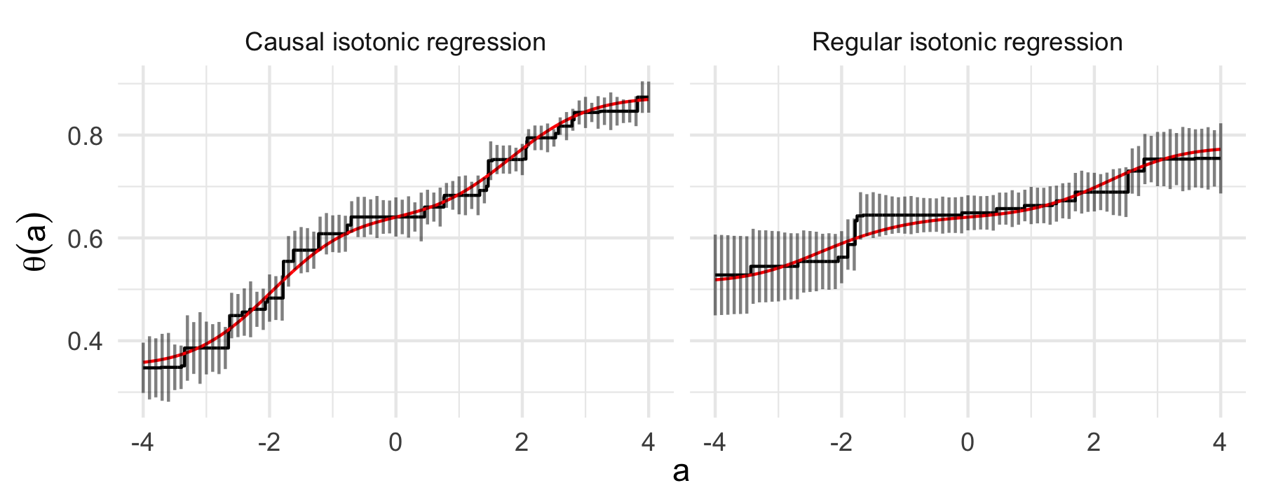
The left panel of Figure 1 shows a single sample path of the causal isotonic regression estimator based on a sample of size and consistent estimators and . Also included in that panel are asymptotic 95% pointwise confidence intervals constructed using the doubly-robust estimator of . The right panel shows the unadjusted isotonic regression estimate based on the same data and corresponding 95% asymptotic confidence intervals. The true causal and unadjusted regression curves are shown in red. We note that for , since the relationship between and is confounded by , and indeed the unadjusted regression curve does not have a causal interpretation. Therefore, the marginal isotonic regression estimator will not be consistent for the true causal parameter. In this data-generating setting, the causal effect of on is larger in magnitude than the marginal effect of on in the sense that has greater variation over values of than does .
We perform 1000 simulations, each with observations. Figure 2 displays the empirical standard error of the three considered estimators over these 1000 simulated datasets as a function of and for each value of . We first note that the standard error of the local linear estimator is smaller than that of , which is expected due to the faster rate of convergence of the local linear estimator. The sample splitting procedure also reduces the standard error of . Furthermore, the standard deviation of the local linear estimator appears to decrease faster than , whereas the standard deviation of the estimators based on do not, in line with the theoretical rates of convergence of these estimators. We also note that inconsistent estimation of the propensity has little impact on the standard errors of any of the estimators, but inconsistent estimation of the outcome regression results in slightly larger standard errors.

Figure 3 displays the absolute bias of the three estimators. For most values of , the estimator proposed here has smaller absolute bias than the local linear estimator, and its absolute bias decreases faster than . The absolute bias of the local linear estimator depends strongly on , and in particular is largest where the second derivative of is large in absolute value, agreeing with the large-sample theory described in Kennedy et al. (2017). The sample splitting estimator has larger absolute bias than because it inherits the bias of . The bias is especially large for values of in the tails of the marginal distribution of .

Figure 4 shows the empirical coverage of nominal 95% pointwise confidence intervals for a range of values of for the four methods considered. For both the plug-in and doubly-robust intervals centered around , the coverage improves as grows, especially for values of in the tails of the marginal distribution of . Under correct specification of outcome and propensity regression models, the plug-in method attains close to nominal coverage rates for between and by . When the propensity estimator is inconsistent, the plug-in method still performs well in this example, although we do not expect this to always be the case. However, when is inconsistent, the plug-in method is very conservative for positive values of . The doubly-robust method attains close to nominal coverage for large samples as long as one of or is consistent. Compared to the plug-in method, the doubly-robust method requires larger sample sizes to achieve good coverage, especially for extreme values of . This is because the doubly-robust estimator of has a slower rate of convergence than does the plug-in estimator, as demonstrated by box plots of these estimators provided in Supplementary Material.
The confidence intervals associated with the local linear estimator have poor coverage for values of where the bias of the estimator is large, which, as mentioned above, occurs when the second derivative of is large in absolute value. Overall, the sample splitting estimator has excellent coverage, except perhaps for values of in the tails of the marginal distribution of when is small or moderate, in which case the coverage is near 90%.

We also conducted a small simulation study to illustrate the performance of the proposed procedures when machine learning techniques are used to construct and . To consistently estimate , we used a Super Learner (van der Laan et al., 2007) with a library consisting of generalized linear models, multivariate adaptive regression splines, and generalized additive models. To consistently estimate , we used the method proposed by Díaz and van der Laan (2011) with covariate vector . To produce inconsistent estimators or , we used the same estimators but omitted covariates and . We also considered the estimator obtained via cross-fitting these nuisance parameters, as discussed in Section 3.7, as well as the local linear estimator. Due to computational limitations, we performed 1000 simulations at sample size only. Figure 5 shows the coverage of nominal 95% confidence intervals. The plug-in intervals achieve very close to nominal coverage under consistent estimation of both nuisances, and also achieve surprisingly good coverage rates when the propensity is inconsistently estimated. The plug-in intervals are somewhat conservative when the outcome regression is inconsistently estimated. The doubly-robust method is anti-conservative under inconsistent estimation of both nuisances and also when the propensity is inconsistently estimated, with coverage rates mostly between 90 and 95%. Good coverage rates are also achieved when the outcome regression is inconsistently estimated. These results suggest that the doubly-robust intervals may require larger sample sizes to achieve good coverage, particularly when machine learning estimators are used for and . The plug-in intervals appear to be relatively robust to moderate misspecification of models for the nuisance parameters in smaller samples. Histograms of the estimators of and are provided in the Supplementary Material. Confidence intervals based on the local linear estimator show a similar pattern as in the previous simulation study, undercovering where the second derivative of the true function is large in absolute value. Cross-fitting had little impact on coverage.
As noted above, we found in our numerical experiments that the plug-in estimator of the scale parameter was surprisingly robust to inconsistent estimation of the nuisance parameters, while its doubly-robust estimator was anti-conservative even when the nuisance parameters were estimated consistently. This phenomenon can be explained in terms of the bias and variance of the two proposed scale estimators. On one hand, under inconsistent estimation of any nuisance function, the plug-in estimator of the scale parameter is biased, even in large samples. However, its variance decreases relatively quickly with sample size, since it is a simple empirical average of estimated functions. On the other hand, the doubly-robust estimator is asymptotically unbiased, but its variance decreases much slower with sample size. These trends can be observed in the figures provided in the Supplementary Material. In sufficiently large samples, the doubly-robust estimator is expected to outperform the plug-in estimator in terms of mean squared error when one of the nuisances is inconsistently estimated. However, the sample size required for this trade-off to significantly affect confidence interval coverage depends on the degree of inconsistency. While we did not see this tradeoff occur at the sample sizes used in our numerical experiments, we expect the benefits of the doubly-robust confidence interval construction to become apparent in smaller samples in other settings.

6 BMI and T-cell response in HIV vaccine studies
The scientific literature indicates that, for several vaccines, obesity or BMI is inversely associated with immune responses to vaccination (see, e.g. Sheridan et al., 2012; Young et al., 2013; Jin et al., 2015; Painter et al., 2015; Liu et al., 2017). Some of this literature has investigated potential mechanisms of how obesity or higher BMI might lead to impaired immune responses. For example, Painter et al. (2015) concluded that obesity may alter cellular immune responses, especially in adipose tissue, which varies with BMI. Sheridan et al. (2012) found that obesity is associated with decreased CD8+ T-cell activation and decreased expression of functional proteins in the context of influenza vaccines. Liu et al. (2017) found that obesity reduced Hepatitis B immune responses through “leptin-induced systemic and B cell intrinsic inflammation, impaired T cell responses and lymphocyte division and proliferation.” Given this evidence of a monotone effect of BMI on immune responses, we used the methods presented in this paper to assess the covariate-adjusted relationship between BMI and CD4+ T-cell responses using data from a collection of clinical trials of candidate HIV vaccines. We present the results of our analyses here.
In Jin et al. (2015), the authors compared the compared the rate of CD4+ T cell response to HIV peptide pools among low (BMI ) medium ( BMI ) and high (BMI ) BMI participants, and they found that low BMI participants had a statistically significantly greater response rate than high BMI participants using Fisher’s exact test. However, such a marginal assessment of the relationship between BMI and immune response can be misleading because there are known common causes, such as age and sex, of both BMI and immune response. For this reason, Jin et al. (2015) also performed a logistic regression of the binary CD4+ responses against sex, age, BMI (not discretized), vaccination dose, and number of vaccinations. In this adjusted analysis, they found a significant association between BMI and CD4+ response rate after adjusting for all other covariates (OR: 0.92; 95% CI: 0.86, 0.98; =0.007). However, such an adjusted odds-ratio only has a formal causal interpretation under strong parametric assumptions. As discussed in Section 1.2, the covariate-adjusted dose-response function is identified with the causal dose-response curve without making parametric assumptions, and is therefore of interest for understanding the continuous covariate-adjusted relationship between BMI and immune responses.
We note that there is some debate in the causal inference literature about whether exposures such as BMI have a meaningful interpretation in formal causal modeling. In particular, some researchers suggest that causal models should always be tied to hypothetical randomized experiments (see, e.g., Bind and Rubin, 2017), and it is difficult to imagine a hypothetical randomized experiment that would assign participants to levels of BMI. From this perspective, it may therefore not be sensible to interpret in a causal manner in the context of this example. Nevertheless, as discussed in the introduction, we contend that is still of interest. In particular, it provides a meaningful summary of the relationship between BMI and immune response accounting for measured potential confounders. In this case, we interpret as the probability of immune response in a population of participants with BMI value but sex, age, vaccination dose, number of vaccinations, and study with a similar distribution to that of the entire study population.
We pooled data from the vaccine arms of 11 phase I/II clinical trials, all conducted through the HIV Vaccine Trials Network (HVTN). Ten of these trials were previously studied in the analysis presented in Jin et al. (2015), and a detailed description of the trials are contained therein. The final trial in our pooled analysis is HVTN 100, in which 210 participants were randomized to receive four doses of the ALVAC-HIV vaccine (vCP1521). The ALVAC-HIV vaccine, in combination with an AIDSVAX boost, was found to have statistically significant vaccine efficacy against HIV-1 in the RV-144 trial conducted in Thailand (Rerks-Ngarm et al., 2009). CD4+ and CD8+ T-cell responses to HIV peptide pools were measured in all 11 trials using validated intracellular cytokine staining at HVTN laboratories. These continuous responses were converted to binary indicators of whether there was a significant change from baseline using the method described in Jin et al. (2015). We analyzed these binary responses at the first visit following administration of the last vaccine dose–either two or four weeks after the final vaccination depending on the trial. After accounting for missing responses from a small number of participants, our analysis datasets consisted of a total of participants for the analysis of CD4+ responses and participants for CD8+ responses. Here, we focus on analyzing CD4+ responses; we present the analysis of CD8+ responses in Supplementary Material.
We assessed the relationship between BMI and T-cell response by estimating the covariate-adjusted dose-response function using our cross-fitted estimator , the local linear estimator, and the sample-splitting version of our estimator with splits. We adjusted for sex, age, vaccination dose, number of vaccinations, and study. We estimated and as in the machine learning-based simulation study described in Section 5, and constructed confidence intervals for our estimator using both the plug-in and doubly-robust estimators described above.
Figure 10 presents the estimated probability of a positive CD4+ T-cell response as a function of BMI for BMI values between the 0.05 and 0.95 quantile of the marginal empirical distribution of BMI using our estimator (left panel), the local linear estimator (middle panel), and the sample-splitting estimator (right panel). Pointwise 95% confidence intervals are shown as dashed/dotted lines. The three methods found qualitatively similar results. We found that the change in probability of CD4+ response appears to be largest for BMI and BMI . We estimated the probability of having a positive CD4+ T-cell response, after adjusting for potential confounders, to be 0.52 (95% doubly-robust CI: 0.44–0.59) for a BMI of 20, 0.47 (0.42–0.52) for a BMI of 25, 0.47 (0.32–0.62) for a BMI of 30, and 0.29 (0.12–0.47) for a BMI of 35. We estimated the difference between these probabilities for BMIs of 20 and 35 to be 0.22 (0.03–0.41).

7 Concluding remarks
The work we have presented in this paper lies at the interface of causal inference and shape-constrained nonparametric inference, and there are natural future directions building on developments in either of these areas. Inference on a monotone causal dose-response curve when outcome data are only observed subject to potential coarsening, such as censoring, truncation, or missingness, is needed to increase the applicability of our proposed method. To tackle such cases, it appears most fruitful to follow the general primitive strategy described in Westling and Carone (2019) based on a revised causal identification formula allowing such coarsening.
It would be useful to develop tests of the monotonicity assumption, as Durot (2003) did for regression functions. Such a test could likely be developed by studying the large-sample behavior of under the null hypothesis that is monotone, where and are the primitive estimator and its greatest convex minorant as defined in Section 2.2. Such a result would likely permit testing with a given asymptotic size when is strictly increasing, and asymptotically conservative inference otherwise. It would also be useful to develop methods for uniform inference. Uniform inference is difficult in this setting due to the fact that does not convergence weakly as a process in the space of bounded functions on to a tight limit process. Indeed, Theorem 3 indicates that converges to an independent white noise process, which is not tight, so that this convergence is not useful for constructing uniform confidence bands. Instead, it may be possible to extend the work of Durot et al. (2012) to our setting (and other generalized Grenander-type estimators) by demonstrating that converges in distribution to a non-degenerate limit for some constant depending upon , a deterministic sequence , and a suitable sequence of subsets increasing to . Developing procedures for uniform inference and tests of the monotonicity assumption are important areas for future research.
An alternative approach to estimating a causal dose-response curve is to use local linear regression, as Kennedy et al. (2017) did. As is true in the context of estimating classical univariate functions such as density, hazard, and regression functions, there are certain trade-offs between local linear smoothing and monotonicity-based methods. On the one hand, local linear regression estimators exhibit a faster rate of convergence whenever optimal tuning rates are used and the true function possesses two continuous derivatives. However, the limit distribution involves an asymptotic bias term depending on the second derivative of the true function, so that confidence intervals based on optimally-chosen tuning parameters provide asymptotically correct coverage only for a smoothed parameter rather than the true parameter of interest. In contrast, monotonicity-constrained estimators such as the estimator proposed here exhibit an rate of convergence whenever the true function is strictly monotone and possesses one continuous derivative, do not require choosing a tuning parameter, are invariant to strictly increasing transformations of the exposure, and their limit theory does not include any asymptotic bias (as illustrated by Theorem 2). We note that both estimators achieve the optimal rate of convergence for pointwise estimation of a univariate function under their respective smoothness constraints. In our view, the ability to perform asymptotically valid inference using a monotonicity-constrained estimator is one of the most important benefits of leveraging the monotonicity assumption rather than using smoothing methods. This advantage was evident in our numerical studies when comparing the isotonic estimator proposed here and the local linear method of Kennedy et al. (2017). Under-smoothing can be used to construct calibrated confidence intervals using kernel-smoothing estimators, but performing adequate under-smoothing in practice is challenging.
The two methods for pointwise asymptotic inference we presented require estimation of the derivative and the scale parameter . We found that the plug-in estimator of had low variance but possibly large bias depending on the levels of inconsistency of and , and that its doubly-robust estimator instead had high variance but low bias as long as either or is consistent. In practice, we found the low variance of the plug-in estimator to often outweigh its bias, resulting in better coverage rates for intervals based on the plug-in estimator of , especially in samples of small and moderate sizes. Whether a doubly-robust estimator of with smaller variance can be constructed is an important question to be addressed in future work. We found that sample splitting with as few as splits provided doubly-robust coverage, and the sample splitting estimator also had smaller variance than the original estimator, at the expense of some additional bias.
It would be even more desirable to have inferential methods that do not require estimation of additional nuisance parameters or sample splitting. Unfortunately, the standard nonparametric bootstrap is not generally consistent in Grenander-type estimation settings, and although alternative bootstrap methods have been proposed, to our knowledge, all such proposals require the selection of critical tuning parameters (Kosorok, 2008; Sen et al., 2010). Likelihood ratio-based inference for Grenander-type estimators has proven fruitful in a variety of contexts (see, e.g. Banerjee and Wellner, 2001; Groeneboom and Jongbloed, 2015), and extending such methods to our context is also an area of significant interest in future work.
References
- Ayer et al. (1955) Ayer, M., H. D. Brunk, G. M. Ewing, W. T. Reid, and E. Silverman (1955). An empirical distribution function for sampling with incomplete information. The Annals of Mathematical Statistics, 641–647.
- Balabdaoui et al. (2011) Balabdaoui, F., H. Jankowski, M. Pavlides, A. Seregin, and J. Wellner (2011). On the Grenander estimator at zero. Statistica Sinica 21(2), 873.
- Banerjee et al. (2019) Banerjee, M., C. Durot, and B. Sen (2019, 04). Divide and conquer in nonstandard problems and the super-efficiency phenomenon. Ann. Statist. 47(2), 720–757.
- Banerjee and Wellner (2001) Banerjee, M. and J. A. Wellner (2001). Likelihood ratio tests for monotone functions. Ann. Stat. 29(6), 1699–1731.
- Bang and Robins (2005) Bang, H. and J. M. Robins (2005). Doubly robust estimation in missing data and causal inference models. Biometrics 61(4), 962–973.
- Barlow et al. (1972) Barlow, R. E., D. J. Bartholomew, J. M. Bremner, and H. D. Brunk (1972). Statistical Inference Under Order Restrictions: The Theory and Application of Isotonic Regression. Wiley New York.
- Belloni et al. (2018) Belloni, A., V. Chernozhukov, D. Chetverikov, and Y. Wei (2018, 12). Uniformly valid post-regularization confidence regions for many functional parameters in Z-estimation framework. Ann. Statist. 46(6B), 3643–3675.
- Bind and Rubin (2017) Bind, M.-A. C. and D. B. Rubin (2017). Bridging observational studies and randomized experiments by embedding the former in the latter. Statistical Methods in Medical Research. Forthcoming.
- Brunk (1970) Brunk, H. D. (1970). Estimation of isotonic regression. In Nonparametric Techniques in Statistical Inference (Proc. Sympos., Indiana Univ., Bloomington, Ind., 1969), London, pp. 177–197. Cambridge Univ. Press.
- Chernoff (1964) Chernoff, H. (1964). Estimation of the mode. Annals of the Institute of Statistical Mathematics 16(1), 31–41.
- Díaz and van der Laan (2011) Díaz, I. and M. J. van der Laan (2011). Super learner based conditional density estimation with application to marginal structural models. The International Journal of Biostatistics 7(1), 1–20.
- Durot (2003) Durot, C. (2003). A Kolmogorov-type test for monotonicity of regression. Statistics & Probability Letters 63(4), 425 – 433.
- Durot et al. (2012) Durot, C., V. N. Kulikov, and H. P. Lopuhaä (2012). The limit distribution of the -error of Grenander-type estimators. The Annals of Statistics 40(3), 1578–1608.
- Gill and Robins (2001) Gill, R. D. and J. M. Robins (2001). Causal inference for complex longitudinal data: The continuous case. The Annals of Statistics 29(6), 1785–1811.
- Groeneboom and Jongbloed (2014) Groeneboom, P. and G. Jongbloed (2014). Nonparametric estimation under shape constraints. Cambridge University Press.
- Groeneboom and Jongbloed (2015) Groeneboom, P. and G. Jongbloed (2015, 10). Nonparametric confidence intervals for monotone functions. The Annals of Statistics 43(5), 2019–2054.
- Groeneboom and Wellner (2001) Groeneboom, P. and J. A. Wellner (2001). Computing Chernoff’s distribution. Journal of Computational and Graphical Statistics 10(2), 388–400.
- Horvitz and Thompson (1952) Horvitz, D. G. and D. J. Thompson (1952). A Generalization of Sampling Without Replacement from a Finite Universe. Journal of the American Statistical Association 47(260), 663–685.
- Jin et al. (2015) Jin, X., C. Morgan, et al. (2015). Multiple factors affect immunogenicity of DNA plasmid HIV vaccines in human clinical trials. Vaccine 33(20), 2347–2353.
- Kennedy (2019) Kennedy, E. H. (2019). Nonparametric Causal Effects Based on Incremental Propensity Score Interventions. Journal of the American Statistical Association 114(526), 645–656.
- Kennedy et al. (2017) Kennedy, E. H., Z. Ma, M. D. McHugh, and D. S. Small (2017). Non-parametric methods for doubly robust estimation of continuous treatment effects. Journal of the Royal Statistical Society: Series B (Statistical Methodology) 79(4), 1229–1245.
- Kosorok (2008) Kosorok, M. R. (2008). Bootstrapping the grenander estimator. In N. Balakrishnan, E. A. Peñ, and M. J. Silvapulle (Eds.), Beyond Parametrics in Interdisciplinary Research: Festschrift in Honor of Professor Pranab K. Sen, Volume 1 of Collections, pp. 282–292. Institute of Mathematical Statistics.
- Kulikov and Lopuhaä (2006) Kulikov, V. N. and H. P. Lopuhaä (2006). The behavior of the NPMLE of a decreasing density near the boundaries of the support. The Annals of Statistics 34(2), 742–768.
- Liu et al. (2017) Liu, F., Z. Guo, and C. Dong (2017). Influences of obesity on the immunogenicity of hepatitis b vaccine. Human vaccines & immunotherapeutics 13(5), 1014–1017.
- Neugebauer and van der Laan (2005) Neugebauer, R. and M. van der Laan (2005). Why prefer double robust estimators in causal inference? Journal of Statistical Planning and Inference 129(1-2), 405–426.
- Neugebauer and van der Laan (2007) Neugebauer, R. and M. J. van der Laan (2007). Nonparametric causal effects based on marginal structural models. Journal of Statistical Planning and Inference 137(2), 419–434.
- Nolan and Pollard (1987) Nolan, D. and D. Pollard (1987). -Processes: Rates of Convergence. Ann. Statist. 15(2), 780–799.
- Painter et al. (2015) Painter, S. D., I. G. Ovsyannikova, and G. A. Poland (2015). The weight of obesity on the human immune response to vaccination. Vaccine 33(36), 4422–4429.
- Rerks-Ngarm et al. (2009) Rerks-Ngarm, S., P. Pitisuttithum, S. Nitayaphan, J. Kaewkungwal, J. Chiu, R. Paris, N. Premsri, C. Namwat, M. de Souza, E. Adams, et al. (2009). Vaccination with ALVAC and AIDSVAX to prevent HIV-1 infection in Thailand. New England Journal of Medicine 361(23), 2209–2220.
- Robins (1986) Robins, J. (1986). A new approach to causal inference in mortality studies with a sustained exposure period – application to control of the healthy worker survivor effect. Mathematical Modelling 7(9), 1393–1512.
- Robins (2000) Robins, J. M. (2000). Marginal structural models versus structural nested models as tools for causal inference. In M. E. Halloran and D. Berry (Eds.), Statistical Models in Epidemiology, the Environment, and Clinical Trials, New York, NY, pp. 95–133. Springer New York.
- Robins et al. (1994) Robins, J. M., A. Rotnitzky, and L. P. Zhao (1994). Estimation of regression coefficients when some regressors are not always observed. Journal of the American Statistical Association 89(427), 846–866.
- Rotnitzky et al. (1998) Rotnitzky, A., J. M. Robins, and D. O. Scharfstein (1998). Semiparametric regression for repeated outcomes with nonignorable nonresponse. Journal of the American Statistical Association 93(444), 1321–1339.
- Rubin and van der Laan (2006) Rubin, D. and M. J. van der Laan (2006). Extending marginal structural models through local, penalized, and additive learning. Working Paper 212, Division of Biostatistics, University of California at Berkeley, Berkeley, California.
- Scharfstein et al. (1999) Scharfstein, D. O., A. Rotnitzky, and J. M. Robins (1999). Adjusting for nonignorable drop-out using semiparametric nonresponse models. Journal of the American Statistical Association 94(448), 1096–1120.
- Sen et al. (2010) Sen, B., M. Banerjee, and M. Woodroofe (2010). Inconsistency of the bootstrap: the Grenander estimator. The Annals of Statistics 38(4), 1953–1977.
- Sheridan et al. (2012) Sheridan, P. A., H. A. Paich, J. Handy, E. A. Karlsson, M. G. Hudgens, A. B. Sammon, L. A. Holland, S. Weir, T. L. Noah, and M. A. Beck (2012). Obesity is associated with impaired immune response to influenza vaccination in humans. International journal of obesity 36(8), 1072.
- van der Laan et al. (2018) van der Laan, M. J., A. Bibaut, and A. R. Luedtke (2018). CV-TMLE for nonpathwise differentiable target parameters. In M. J. van der Laan and S. Rose (Eds.), Targeted Learning in Data Science: Causal Inference for Complex Longitudinal Studies, pp. 455–481. Springer.
- van der Laan et al. (2007) van der Laan, M. J., E. C. Polley, and A. E. Hubbard (2007). Super learner. Statistical Applications in Genetics and Molecular Biology 6(1).
- van der Laan and Robins (2003) van der Laan, M. J. and J. M. Robins (2003). Unified methods for censored longitudinal data and causality. Springer Science & Business Media.
- van der Laan and Rose (2011) van der Laan, M. J. and S. Rose (2011). Targeted learning: causal inference for observational and experimental data. Springer-Verlag New York.
- van der Vaart and van der Laan (2006) van der Vaart, A. W. and M. J. van der Laan (2006). Estimating a survival distribution with current status data and high-dimensional covariates. The International Journal of Biostatistics 2(1).
- van der Vaart and Wellner (1996) van der Vaart, A. W. and J. A. Wellner (1996). Weak Convergence and Empirical Processes. Springer.
- Westling and Carone (2019) Westling, T. and M. Carone (2019). A unified study of nonparametric inference for monotone functions. Ann. Stat.. to appear.
- Westling et al. (2018) Westling, T., M. van der Laan, and M. Carone (2018). Correcting an estimator of a multivariate monotone function with isotonic regression. arXiv e-prints, arXiv:1810.09022.
- Woodroofe and Sun (1993) Woodroofe, M. and J. Sun (1993). A penalized maximum likelihood estimate of f(0+) when f is non-increasing. Statistica Sinica 3(2), 501–515.
- Young et al. (2013) Young, K. M., C. M. Gray, and L.-G. Bekker (2013). Is obesity a risk factor for vaccine non-responsiveness? PloS one 8(12), e82779.
- Zhang et al. (2016) Zhang, Z., J. Zhou, W. Cao, and J. Zhang (2016). Causal inference with a quantitative exposure. Statistical Methods in Medical Research 25(1), 315–335. PMID: 22729475.
- Zheng and van der Laan (2011) Zheng, W. and M. J. van der Laan (2011). Cross-validated targeted minimum loss based estimation. In M. van der Laan and S. Rose (Eds.), Targeted learning: causal inference for observational and experimental data, Chapter 27, pp. 459–473. New York: Springer-Verlag New York.
Supplementary material: technical results
We will use the notation to refer to for any probability measure and -integrable function . We will denote by the empirical distribution based on , so that . We will denote by the empirical process . Finally, we will say that if there exists a such that . Below, for brevity, we will refer to Westling and Carone (2019) as WC.
Throughout the Supplementary Material, we will refer to as any element of at which we evaluate functions such as , , or . We will reserve for arguments to integrands and influence functions.
Supporting lemmas
Before proceeding to proofs for Theorems 1 and 2, we state three lemmas that we will use. First, we derive a first-order expansion of that we will rely upon. We define with
and . We also define
We then have the following first-order expansion.
Lemma 6.
If condition (A3) holds, then , where we have defined with
Proof.
We define
so that . By (A3), we have that
Thus, we have the expansion for . By adding and subtracting terms and rearranging, we can write as follows:
The sum of the first and third lines in the preceding display can be expressed as . Therefore, we can decompose the remainder term into as claimed, where
Furthermore, can be rewritten as claimed by adding and subtracting terms. ∎
Lemma 7 below indicates that the entropy of a uniformly bounded class over a product space, when marginalized over one component of the product space with respect to a fixed probability measure, is bounded above by the entropy of the original class.
Lemma 7.
Let be a uniformly bounded class of functions , with for all . Let be a fixed probability measure on , and define . Then, we have that
Proof.
The statement follows immediately from Lemma 5.2 of van der Vaart and van der Laan (2006) by taking . ∎
The final lemma concerns so-called degenerate U-processes, and is a slight extension of Theorem 6 of Nolan and Pollard (1987). A -degenerate -process for a class of functions is defined as a sum of the form , where
and where each is a function from satisfying that: (i) is symmetric in its arguments, meaning that for all , and (ii) for all . For such processes, we have the following result.
Lemma 8.
Suppose be a -degenerate -process. If is an envelope function for , then we have that
Proof.
We let , and also define , and , where
Theorem 6 of Nolan and Pollard (1987) then states that
Now, we note that
where the supremum is taken over all finite, discrete such that . Next, since , we have
By Jensen’s inequality, we have that , which then implies the claimed result.
∎
Proof of Theorem 1
We use Theorem 1 of WC for both the pointwise and uniform consistency statements. Since is the empirical distribution function, by the Glivenko-Cantelli Theorem. Hence, we only need to show that .
We first establish that is a -Donsker class. The class is a VC class and hence also -Donsker. Since is a bounded, fixed function, is also -Donsker, which implies that is -Donsker by Lemma 7. Hence, by the permanence properties of Donsker classes, we find that is a -Donsker class and thus that .
We first focus on studying remainder term , which can be uniformly bounded by
By assumption, , and since is eventually bounded uniformly above and away from zero almost surely, as well. Also, and since , , and are all bounded for large enough. Hence, .
For the remainder term , we define the stochastic process . We will use Lemma 4 of WC to establish that . In their notation, we set , equipped with the usual Euclidean norm, and , equipped with the product semi-metric . Application of this result requires showing that the process is uniformly asymptotically -equicontinuous for the product semi-metric. This would be implied if the class were -Donsker. Note that condition (A1) implies that and are -Donsker classes by Theorem 2.5.2 of van der Vaart and Wellner (1996). Since is a -Donsker, as established above, the classes and are also -Donsker by Lemma 7. Since is bounded below, the class is also -Donsker. This then yields that the original class is -Donsker. The second requirement of Lemma 4 of WC is satisfied by assumption.
Finally, we analyze the remainder term , which itself has three components, as decomposed before the presentation of Lemma 7. Its second component is an ordinary empirical process involving function classes discussed in the preceding paragraph. Using these results yields the second component to be . Its third sub-component is a bias term which, in view of the uniform boundedness of , is . Its first sub-component is a -degenerate -process as defined above, to which we will apply Lemma 8. The function is contained in the class . As we discuss in more detail below, by Lemma 7 and Lemma 5.1 of van der Vaart and van der Laan (2006), and in view of condition (A1), this class has uniform entropy bounded up to a constant by relative to a constant envelope. Therefore, Lemma 8 implies that
Therefore, the first sub-component of is . Thus, we have that .
In conclusion, we have shown that conditions (A1)–(A3) imply that all three remainder terms are controlled, so that . ∎
Proof of Theorem 2
We will use Theorem 4 of WC to establish Theorem 2 stated in the main text. In what follows, we verify conditions (B1)–(B5) and (A4)–(A5) of WC, which we refer to as (WC.B1), (WC.B2) and so on.
Conditions (WC.B1) and (WC.B2).
Define pointwise and . Since is by assumption strictly increasing at , we then have that
where we define .
The class is a VC class of functions by a slight extension of Example 2.6.1 of van der Vaart and Wellner (1996). Its envelope function is , and hence, we have that by Theorem 2.6.7 of van der Vaart and Wellner (1996). The class thus satisfies the same inequality by Lemma 7. The classes , and are sets of constants not depending on the data, bounded up to a constant by for small enough since and are continuously differentiable in a neighborhood of . Hence, they also have uniform entropy bounded up to a constant by . Finally, the class is a linear combination of the above classes, and so, by Lemma 5.1 of van der Vaart and van der Laan (2006), satisfies that as well. This verifies condition (WC.B1).
Since , and are continuously differentiable in a neighborhood of , an envelope function for the class is
for some . Using the triangle inequality on , we first note that
for some by the boundedness of , , , and the conditional density in a neighborhood of uniformly over almost every under . Similar bounds hold for the other terms, yielding that for all small enough, as required.
For the second requirement of (WC.B2), we note that for all small enough and some constants . By assumption, and in view of properties of probability densities, for all small enough and for all , there is a such that . This implies that for any , for all small enough.
Condition (WC.B3).
Next, we need to study the covariance for near , where , and where we may ignore any terms in the covariance function that are continuously differentiable in a neighborhood of . We thus have
Since , and are continuously differentiable in a neighborhood of , expanding , it is straightforward to see that we may focus on
The bottom three lines are continuously differentiable in in a neighborhood of since , , and are all continuous in a neighborhood of , uniformly over almost every under . As such, they do not contribute to the scale parameter of the limit.
By Fubini’s theorem, the first line can be rewritten as
In view of (A5), this satisfies (WC.B3), and so, the limit distribution is , where
We can thus simplify the scale factor to , where is as defined in the statement of Theorem 2.
Conditions (WC.B4) and (WC.B5).
Defining
for each , we must show that for all small enough and that, for some , is decreasing for all small enough and large enough. For , by Fubini’s theorem and taking supremum bounds, for large enough and small enough, we find that
Hence, under conditions (A4a), (A4b) and (A4c), for each . Furthermore, is decreasing for any by the assumed uniform boundedness of , , , , and .
We will use Theorem 6 of WC to establish negligibility of the empirical process term , which requires checking conditions (WC.C1)–(WC.C4). Let , which is contained in the product class almost surely for all large enough, itself equipped with the semi-metric
Next, we define , where
We let be the envelope function for obtained by combining the assumed uniform bounds on and along with the natural envelope for . Specifically, we have for some . For all small enough and some , is a Lipschitz transformation of the following classes:
- •
, which has uniform entropy bounded up to a constant by ;
- •
, which has uniform entropy bounded up to a constant by ;
- •
, which has uniform entropy bounded up to a constant by in view of Lemma 7;
- •
, which has polynomial covering number;
- •
, which has uniform entropy bounded up to a constant by in view of Lemma 5.1 of van der Vaart and van der Laan (2006) and our Lemma 7;
- •
, which has polynomial covering number;
- •
the singleton class , with covering number equal to one.
Thus, by Lemma 5.1 of van der Vaart and van der Laan (2006), the covering number of relative to is bounded up to a constant by . Since , is uniformly bounded above for all small enough with probability tending to one. This establishes (WC.C1).
Existence of the conditional variance of given and positivity of in a neighborhood of yields that and that, for any , there exists such that for all small enough. Hence, condition (WC.C2) is satisfied.
Turning to (WC.C3), we note that is bounded above by
and by the finite conditional second moment of given , the boundedness of , the uniform boundedness of and , and the positivity of near , we find that for all in a neighborhood of 0. Similarly, we can bound above by
We find that, for small enough, this is bounded up to a constant by
as required. Finally, (WC.C4) is satisfied by assumption.
For , we first note that (WC.B4) has already been shown to hold in the proof of Theorem 4, since
We verify (WC.B5) for each of the three sub-components of defined by the three sub-components of . Due to the assumed boundedness of , the contribution of the third component is bounded for all small enough up to a constant (not depending on or ) by , which satisfies (WC.B5). For the second component, by Lemma 4 of WC, , and so, the expectation of the second component is bounded up to a constant by for all small enough and large enough, which is also sufficient for (WC.B5).
The first component requires controlling , where we define
The function falls in the class . Thus, is a -degenerate -process. By a similar argument as made above, the class has uniform entropy bounded up to a constant by relative to the envelope
Since and , Lemma 8 yields that
for all small enough. Hence, (WC.B5) is satisfied for this -process term.
Conditions (WC.A4) and (WC.A5).
Condition (WC.A4) is trivially satisfied since the transformation used here is the empirical distribution function. Condition (WC.A5) was established in the proof of Theorem 1 under our conditions (A1)–(A3). We have now checked all the conditions of Theorem 4 of WC and verified the stated limit distribution in the course of checking condition (WC.B3). This concludes the proof. ∎
Proof of Theorem 3
We first note that and if and only if and . By Lemma 1 of WC, this holds if and only if the set of inequalities
holds true. Standard manipulation of the argmax (see the proof of Theorem 3 of WC) yields that this is equivalent to the set of inequalities
where we have defined the terms
We have that for and any by uniform consistency of , and similarly for and using the continuous differentiability of and differentiability of at and . See the proof of Theorem 3 of WC for additional details.
The core of the argument is to demonstrate that and converge jointly (as processes) to independent Brownian motions and , where and are two independent standard two-sided Brownian motions originating from zero. If this holds, it would follows that
in for all , where . An adaptation of the argmax continuous mapping theorem (i.e. Theorem 3.2.2 of van der Vaart and Wellner (1996)) and the arguments of Theorem 3 of WC imply that under the stated conditions,
where . Since and are independent, so are and , and
From there, standard manipulations of Brownian motion yield the result (see, for example, the proof of Theorem 3 of WC) applied to each and separately.
We now show that and converge jointly as processes to independent Brownian motions and . We note that
for by our derivations in the proof of Theorem 2. Furthermore, since is Lipschitz in neighborhoods of and , we have
for , where we define . Now, for all , for all such that and . Thus, for all such and , and depend on disjoint sets of the observations , which implies that they are independent. This implies that and are independent for all , and hence asymptotically independent for all . Furthermore, the proof of Theorem 4 of WC demonstrates that conditions WC.B1–WC.B4 and WC.A4–WC.A5 imply that the processes for converge marginally as processes in to . Therefore, by Example 1.4.6 of VW, the two processes converge jointly to independent Brownian motions. We have thus found that
for , where and converge jointly to independent Brownian motions. Therefore, and converge jointly to this same limit. ∎
First-order expansion of cross-fitted estimator
Next, we provide proofs of Theorems 4 and 5 for the estimator , which is based upon the cross-fitted nuisance estimators and . We recall that is the training set for fold , that is, the subset of observations in used to estimate and , and is the vector of indices of the validation set for fold , that is, . We note that and for each . We denote by the empirical measure corresponding to the observations with indices in , and we let and denote the marginal empirical measures of and .
Before proving our results, we derive a first-order expansion of that we will rely upon.
Lemma 9.
If condition (A3) holds, then , where for
where is as defined in the proof of Theorem 1.
Proof.
We define
so that . Writing , in view of condition (A3), we have that
The expansion follows by adding and subtracting terms. ∎
Proof of Theorem 4
As before, we use Theorem 1 of WC for both the pointwise and uniform consistency statements. We only need to show that .
In the proof of Theorem 1, we established that . Since the analysis of the remainder term is entirely analogous to that provided in the proof of Theorem 1, we begin by looking at the remainder term instead. We define . We then have . We will demonstrate that using Theorem 2.14.2 of VW. By the tower property,
Here, the inner expectation is with respect to the distribution of the observations in the validation sample given the training sample , while the outer expectation is with respect to the observations in the training sample. Since and are constructed only using , they are fixed when conditioning on . We note that with probability one, for all large enough,
for all . We then define pointwise by taking to be the sum of terms on the right-hand side of the last inequality above. ultimately serves as an envelope function for , so that by Theorem 2.14.1 of VW we have that, for large enough,
for a universal constant , where is the uniform entropy integral as defined in Chapter 2.14 of VW. The class is a convex combination of the class , which is well-known to be VC and hence possess polynomial covering numbers, plus the class for and (both of which are fixed functions), so in view of Lemma 7 this class also possesses polynomial covering numbers. Thus, is uniformly bounded for all and . It follows then that, for some constant and large enough ,
It remains to demonstrate that . We have that is bounded above by
Both terms tend to zero in probability by condition (B2), and since all involved terms are uniformly bounded by condition (B1), they also tend to zero in expectation. Therefore, we have that , which implies that .
Finally, we analyze the remainder term , which itself has three subcomponents, as decomposed before the presentation of Lemma 7. Its second subcomponent, , is an ordinary empirical process and can be analyzed in a manner analogous to that used for . Doing so yields that the second subcomponent is . The third subcomponent of is a bias term which, in view of the uniform boundedness of and , is . The first subcomponent of is a -degenerate -process as defined above. We denote and . We then have As before, we begin by conditioning on so that is a fixed function:
We apply Lemma 8 to the inner expectation. First, we note that is a uniformly bounded class of functions by the uniform boundedness of . Second, the class can be formed as a sequence of compositions of the class , which, as discussed above, has polynomial uniform entropy numbers. This implies that the uniform entropy integral in the upper bound of Lemma 8 is finite. Therefore, we have that
for some universal constant. Thus, the first subcomponent of is also , and we conclude that .
We have now shown that, under conditions (B1)–(B2) and (A3), all three remainder terms are at least , and thus, Theorem 1 of WC yields the result. ∎
Proof of Theorem 5
As before, we use Theorem 4 of WC to establish the result. Verification of the conditions (WC.B1)–(WC.B3) and (WC.A4)–(WC.A5) is identical as in the proof of Theorem 2. Hence, we focus on conditions (WC.B4)–(WC.B5). Specifically, defining
for each , we must show that for all small enough and that, for some , is decreasing for all small enough and large enough. Verification for the term is nearly identical to the analysis presented for in the proof of Theorem 2. For , we first define
for each , where we have suppressed dependence on . We then have that
As before, we condition on , and write
Thus, and are fixed with respect to the inner expectation. We note that
We will take as envelope function for the sum of terms on the right-hand side of the last inequality above, with replaced by . We then have by Theorem 2.14.1 of VW that
The class is once again contained in a sequence of Lipschitz transformations of the class and various fixed functions, so that the class has polynomial uniform entropy numbers and is uniformly bounded for all . We then have for some that
By the boundedness condition (B1), for all large enough, we have that
Since all terms involved are uniformly bounded, we therefore have
so that for each and is decreasing for any and all large enough.
For , we first note that (WC.B4) has already been shown to hold in the proof of Theorem 1, since
We verify (WC.B5) for each of the three subcomponents of defined by the three subcomponents of . Due to the assumed boundedness of and , the contribution of the third subcomponent is bounded for all small enough up to a constant (not depending on or ) by , which satisfies (WC.B5). For the second subcomponent, which is an ordinary empirical process term, analogous methods to that used for can be used to verify (WC.B5). The first subcomponent requires controlling , where we define
Conditioning upon , becomes fixed, so that the function falls in the class for all . Thus,
is a -degenerate -process conditional on . The class has uniform entropy bounded up to a constant by relative to the envelope
Since , Lemma 8 yields that
for all small enough. Hence, (WC.B5) is satisfied for this -process term. ∎
Supplementary material: additional simulation results
Figure 7 presents boxplots of the estimator of the true derivative for each combination of nuisance function estimators used. The estimators are taken to the one-third power because that is what appears in the estimator of the pointwise confidence intervals. The estimators are roughly centered around the truth (shown in red), except for values of in the tails of the distribution of .

Figure 8 shows histograms of the plug-in estimator of . The estimators are taken to the one-third power because that is what appears in the estimator of the pointwise confidence intervals. The estimators are centered around the truth (show in red) when both and are consistent, but are biased for some values of when either or is inconsistent.

Figure 9 shows histograms of the doubly-robust estimator of . Once again, the estimators are taken to the one-third power because that is what appears in the estimator of the pointwise confidence intervals. In all settings considered, the estimators are roughly centered around the truth, which is shown in red. However, the spread of the estimator around the true scale is substantially larger than that of the plug-in estimator.

Supplementary material: additional data analyses
Figure 10 presents the estimated probability of a positive CD8+ T-cell response as a function of BMI for BMI values between the 0.05 and 0.95 quantile of the marginal empirical distribution of BMI using our estimator (left panel), the local linear estimator (middle panel), and the sample-splitting estimator (right panel). Pointwise 95% confidence intervals are shown as dashed/dotted lines.
