Deep Diffeomorphic Normalizing Flows
Hadi Salman Microsoft Research AI hasalman@microsoft.com Payman Yadollahpour University of Pittsburgh payman@pitt.edu Tom Fletcher Universrity of Virginia ptf8v@virginia.edu Kayhan Batmanghelich University of Pittsburgh kayhan@pitt.edu
Abstract
The Normalizing Flow (NF) models a general probability density by estimating an invertible transformation applied on samples drawn from a known distribution. We introduce a new type of NF, called Deep Diffeomorphic Normalizing Flow (DDNF). A diffeomorphic flow is an invertible function where both the function and its inverse are smooth. We construct the flow using an ordinary differential equation (ODE) governed by a time-varying smooth vector field. We use a neural network to parametrize the smooth vector field and a recursive neural network (RNN) for approximating the solution of the ODE. Each cell in the RNN is a residual network implementing one Euler integration step. The architecture of our flow enables efficient likelihood evaluation, straightforward flow inversion, and results in highly flexible density estimation. An end-to-end trained DDNF achieves competitive results with state-of-the-art methods on a suite of density estimation and variational inference tasks. Finally, our method brings concepts from Riemannian geometry that, we believe, can open a new research direction for neural density estimation.
1 Introduction
Efficient computation of the posterior distribution is one of the main problems in Bayesian Inference. The exact form of the posterior density function requires the estimation of the marginal likelihood which is computationally prohibitive in general (Valiant, 1979). To approximate the posterior distribution, there are, arguably, two families of approaches: (1) methods based on sampling (e.g., MCMC (Metropolis et al., 1953; Hastings, 1970), Gibbs (Geman and Geman, 1984), etc.), and (2) variational inference (VI) techniques (Jordan et al., 1999). The general idea of a sampling method is to construct an ergodic chain of the latent variable sampled from the posterior. Although MCMC methods provide asymptotic guarantees for producing exact samples from the posterior (Robert and Casella, 2004), they tend to be computationally expensive for large datasets or complex models.
Instead of sampling, VI techniques convert the approximation problem into an optimization problem. They maximize a lower bound that indirectly minimizes the Kullback-Leibler (KL) divergence between the exact posterior and a member of a postulated family of probability density functions (Jordan et al., 1999; Bishop, 2006). Although no asymptotic guarantee is known for VI, it tends to scale better than MCMC thanks to powerful optimization techniques such as stochastic gradient descent (Robbins and Monro, 1951). The choice of the family of the distribution is important, and a not rich enough family can result in a biased approximation of the posterior (Turner and Sahani, 2011).
In recent years, various neural density estimators have been proposed (Mnih and Gregor, 2014; Rezende and Mohamed, 2015; Kingma et al., 2016; Larochelle and Murray, 2011; Papamakarios et al., 2017; Huang et al., 2018). These methods use neural networks to specify flexible families of distributions for VI. The challenge is to ensure that the approximate densities are easy to sample from and to evaluate. For example Rezende and Mohamed (2015) apply a series of invertible transformations on a random variable drawn from a fixed distribution (e.g., a Gaussian distribution) to represent complex distributions. Larochelle and Murray (2011) use an autoregressive approach which views the approximate posterior as a decomposition of a chain of conditional distributions. Kingma et al. (2016) show that those approaches are closely related.
We propose a novel normalized flow method where the invertible function is a diffeomorphism, dubbed DDNF. A diffeomorphism is an invertible mapping where both the function and its inverse are smooth. Inspired by the literature of large deformation diffeomorphic metric mapping in medical image registration (Beg et al., 2005a; Beg et al., 2005b; Younes, 2010; Zhang and Fletcher, 2015), we use an ODE to construct such a mapping. We propose to use an RNN to discretize the ODE where the RNN cell has a residual neural network (ResNet) (He et al., 2015) architecture. The resulting flow can be viewed as a composition of tiny mappings that are close to the identity transformation. Generalizing some previous methods (Rezende and Mohamed, 2015; Jankowiak and Karaletsos, 2018), DDNF is highly flexible and easy to sample from. The construction of the inverse flow, required for evaluating the likelihood of given data samples at test time, is expressive and straightforward. We draw a connection between neural density estimation and the Riemannian geometric structure of the manifold of diffeomorphic functions which we believe can potentially open new directions of research.11 1 Upon publication, we will open source the code.
2 Background
Given a dataset , the maximum likelihood principle is typically used to learn the parameters of a model given its probability distribution:
Unfortunately, maximum likelihood estimation is computationally expensive in the presence of latent variable because evaluating the objective function entails marginalizing out , i.e., , which is not tractable in general. Instead, VI (Jordan et al., 1999) maximizes a lower bound constructed by an approximation of the posterior, ,
The bound is called the Evidence Lower Bound (ELBO) which is a unified cost function and the parameters of the approximate posterior . The choice of is crucial, and a “not complex enough” distribution can result in a biased estimation of Turner and Sahani (2011). Using a neural network to parameterize has proven to be successful and, with the advent of variational auto-encoders (VAEs) (Kingma and Welling, 2013), has resulted in a new direction of research. The VAE models as a Gaussian distribution with diagonal covariance, i.e., where the mean and variance are a non-linear function of . However, the typically used family of the approximate distribution is limited since it represents a uni-modal distribution given . Rezende and Mohamed (2015) proposed more flexible family of distributions. The idea is to model the posterior as a series of invertible transformations applied to random variables drawn from an initial distributions . A neural network is used to parameterize the transformations. Assuming and , the distribution of , follows,
| (1) |
After applying transformations to the latent variable, i.e., , the variational objective can be written as:
| (2) |
The main challenge is to design a neural network architecture for that is invertible and whose determinant of the Jacobian is easy to compute. Rezende and Mohamed (2015) proposed a family of such transformations named planar normalizing flows: . The function is invertible under a simple constraint and has a closed-form determinant of the Jacobian.
The planar transformation is a single layer neural network and has a limited capacity. Recently, several other methods were introduced to increase the flexibility of the flow while maintaining the invertibility (van den Berg et al., 2018; Huang et al., 2018; Tomczak and Welling, 2016) (see Section 4 for more details), and many novel architectures are proposed to keep the computation of the determinant of the Jacobian tractable. In this paper, we propose to use a special class of invertible mapping called diffeomorphisms which has many appealing mathematical properties.
3 Diffeomorphic Normalizing Flow
In this paper, we enforce the mapping to be diffeomorphic, meaning exists and both and are differentiable. In Section 3.1, we provide some background on the space of diffeomorphisms and how they can be expressed by ordinary differential equations (ODEs). In Section 3.2, we introduce a neural network implementation of the diffeomorphic flow (DDNF), and we present efficient implementations of the determinant of the Jacobian and the inverse of the flow. Finally, in Section 3.3, we propose a few regularization methods that improve the performance of DDNF.


3.1 Background on Diffeomorphisms
In this section, we briefly review the mathematical background for diffeomorphic transformations. Throughout this paper, denotes a mapping defined on a domain . We use to denote the Hilbert space of vector fields on whose derivatives up to order exist and are square-integrable, and where denotes the tangent bundle of . In this paper, we consider diffeomorphisms generated by the flow of time-varying velocity fields. More specifically, given a time-varying vector field , we define the time-varying flow, , as a solution of the following differential equation:
| (3) |
where is a smooth function defining a velocity vector at time over its domain. As shown in Trouvé (1995), integration up to unit time (i.e., ) results in a diffeomorphism if is sufficiently smooth (Rossmann, 2002; Beg et al., 2005b; Beg et al., 2005a; Hauser and Ray, 2017; Younes, 2010). Furthermore, the determinant of the Jacobian of this diffeomorphic flow is guaranteed to be always non-negative (Gordon, 1972).
We represent the time-varying velocity field, , by segments of stationary velocity fields, meaning that the velocity is time invariant within each segment. Hence, the overall flow is a composition of the flows governed by stationary fields. The idea is show in Figure 1.
The space of diffeomorphic transformations () has several appealing properties: (1) it forms an algebraic group that is closed under the composition operation (i.e., if then ) (Hauser and Ray, 2017), (2) with a proper definition of local inner product, all diffeomorphic transformations reside on a Riemannian manifold (Younes, 2010). The second property allows us to define a distance metric and a notion of shortest path between two flows on the manifold. We use notion of the the shortest path as a natural regularization technique of DDNF.
3.2 Neural Network Parametrization
3.2.1 Stationary Velocity Field
In this section, we restrict the diffeomorphisms to a special class where the velocity field in Eq. 3 is time independent (i.e., ). Such restriction, also applied by Arsigny et al. (2006); Arsigny (2006); Vercauteren et al. (2007), defines a subgroup of diffeomorphisms governed by the stationary ODE,
| (4) |
The solution of this ODE is the exponential map of the vector field, i.e., . To compute the exponential map, we adopt an Euler integration approach that composes infinitesimal flow fields successively. In other words, the exponential map can be viewed as a composition of small flows, . Discretizing Eq. 4 over time, we arrive at,
| (5) |
We use an RNN to model Eq. 5 as shown in Figure 2-Middle. Each cell has a ResNet architecture as shown in Figure 2-Top. In order to set , the RNN should be unfolded times. We use a deep neural network as a general parameterization for inside ResNet.
3.2.2 Computation of Determinant Jacobian
Our DDNF applies a series of transformations to a random variable. In order to compute the probability density function of the transformed random variable, the computation of the determinant of the Jacobian () of each transformation is required. The computational complexity of the determinant of the Jacobian of the entire flow is where is the number of cells in the flow and is the dimension of the vector field. Each cell of DDNF applies a small transformation to the random variable. In other words, for , can be viewed as
| (6) |
Each is a identity-like transformation; hence we can use the Taylor series expansion around the identity to approximate the determinant of the Jacobian (see Appendix D for derivation) as follows,
| (7) | ||||
A naive storage cost of the trace is , but the cost can be reduced by a randomized method (Hutchinson, 1990; Maclaurin, 2016) as follows,
| (8) |
which requires efficient Jacobian vector computation resulting in a cost reduction of the original determinant from to .
3.2.3 Inversion of the Flow
Invertibility of the flow enables us to evaluate the posterior distribution of any given latent variable . Not all NFs has straightforward inversion. Previous approaches, such as the planar NF (Rezende and Mohamed, 2015), construct each cell to be invertible by imposing constraints on the parameters of the neural network. However, we construct our flow as an exponential map with no constraint on the neural network. In our approach, the inverse flow is obtained by integrating the negative velocity field in time (Rossmann, 2002), i.e., . In other words, the inverse flow is another DDNF implementing the ODE with . As the number of cells increases (i.e., ), the accuracy of the approximate ODE also increases, resulting in a more accurate inversion of the flow.
3.2.4 Extension to the Time-Varying Velocity Field
The stationary velocity field in Section 3.2.1 is implemented as a series of ResNet cells sharing the same parameters composing one RNN block. Extending the method to time-varying velocity fields is straightforward; we divide the unit interval into segments. For each segment, we use a stationary velocity block with a different set of parameters. Therefore, the resulting architecture is a non-stationary velocity block as shown in Figure 2-Bottom.
3.3 Regularizing the Flow
The structure of our flow suggests two interesting regularizations that improve its performance and stability: (1) geodesic regularization and (2) an inverse consistency regularization.
3.3.1 Geodesic regularization
The is the final point of a path defined by the ODE which is parametrized by a time-varying . There are infinite paths (’s) connecting to . The length of the path indicates a distance of from the identity mapping (i.e., ) on . One may define the optimal velocity field as being the one with minimum path-length, , defined as,
| (9) |
where is a Hilbert norm. We define using the inner product on the space of velocities, :
| (10) |
where is a positive definite operator. In this paper, we simply choose to be the identity operator. To implement the integral in Eq. 9, we use the sum of the -norm of the velocity vectors of cells as a regularizer (see the Appendix E for more choices of the regularizer).


3.3.2 Inverse Consistency Regularization
We use Euler discretization for the integration of the ODE in Eq. 3. The quality of flow inversion increases with the number of cells (i.e., ). However, a large number of cells increases the computational cost for the forward and the backward passes. The geodesic regularization (Eq. 9) improves both the quality of the ODE and approximations but a strong regularization of the velocity field results in a stiff flow (i.e., ). To improve the quality of the inversion, we propose an inverse consistency regularization. For an invertible flow, where is the sample from the initial distribution and is the final output of the forward flow (i.e., ). The proposed regularization enforces them to be close,
| (11) |
The general idea is shown in Figure 3.
4 Related Works
Compared to traditional VI, neural density estimators offer a richer family of approximate posterior distributions. Neural density estimators mainly include two families: normalizing flows (NF) (Rezende and Mohamed, 2015) and autoregressive flows (AF) (Larochelle and Murray, 2011; Uria et al., 2016). In the former group of methods, the goal is to find an invertible function that transforms a random variable drawn from a base density (e.g., a standard Gaussian) to a target density. In addition to the invertibility, the function should have a tractable determinant of the Jacobian. In the latter group, the target density is modeled as the product of conditional densities. Several works drew connections between the two families (Kingma et al., 2016; Papamakarios et al., 2017; Huang et al., 2018).
To model a density, , of a random variable, , in a high dimensional space, an AF first assumes an ordering between coordinates of the variable and models the conditional distribution of , given the previous coordinates, , as . This recursive formulation can be modeled by a recurrent architecture (Uria et al., 2013) where the conditional distributions are assumed to be a function of a hidden state. The dependency on the ordering of the random variables is one of the drawbacks of the AF (see Papamakarios et al. (2017) for an illustration) and several methods are proposed to alleviate the problem (Germain et al., 2015; Papamakarios et al., 2017). Also, in a high dimensional space, generating samples can be expensive (van den Oord et al., 2016). Unlike AFs, our method is not dependent on an ordering, and sampling is relatively inexpensive. Our architecture uses an RNN and may have some resemblance with the AF methods, but the RNN in our method approximates the integration of an ODE and not a conditional distribution.
Our approach is closer to the NF. An NF method starts with random draws from a known distribution and applies a chain of invertible transformations ,
The main challenge is to ensure that is invertible and the determinant of its Jacobian can be efficiently computed. NFs were first introduced by Rezende and Mohamed (2015). They proposed a planar transformation, where and is a non-linearity. is invertible under some constraints (see the Appendix of Rezende and Mohamed (2015) for more details). However, the planar family is limited to an MLP with a single node bottleneck layer. Tomczak and Welling (2016) and van den Berg et al. (2018) proposed models belonging to a volume preserving family. The volume preserving family has limitations in modeling multi-modal densities.
Papamakarios et al. (2017) and Kingma et al. (2016) drew connections between NF and AF. To keep the computation of determinant of Jacobian tractable, they use an affine form between and which results in a lower triangular Jacobian whose determinant is very cheap to compute. Huang et al. (2018) recently proposed Neural Autoregressive Flow (NAF) which extends the previous two papers by replacing the affine transformation with a more rich family of transformation. They ensures the invertibility of the flow by using a monotonic function on the bottleneck layer. Although the resulting flow is invertible, to the best of our knowledge, computing the inverse is not straightforward. Alternatively, we do not have any constraint on the architecture of the MLP and we are able to invert the flow simply by integrating the velocity field backward.
Very recently, Chen et al. (2018) proposed a continuous time RNN based on an ODE solver which can be used as a building block for NF. While we use the Euler method, they propose to use the Runge–Kutta method (Dormand and Prince, 1980) which results in more accurate integration. Integrating their method with ours can improve the performance of our model, but we will leave this for future work. Finally, there are several works at the intersection of deep learning and ODE/PDE (Long et al., 2017; Haber and Ruthotto, 2018) that are tangentially related to our work, and their proposed methods can potentially improve the performance of our diffeomorphic flow.
5 Experimental Results
In this section, we evaluate the proposed method in four different experiments: (1) Forward and Backward Flows, in which we evaluate the accuracy of the forward and backward passes of the flows in approximating the solution of an ODE defined in Section 3. (2) Expressiveness of DDNF, where we study the expressiveness power of the our method on two toy distributions and compare the results with the state-of-the-art and traditional sampling techniques (e.g., MCMC). (3) Effect of Regularization, where we study the effect of the regularizers introduced in Section 3.3 on our flow. (4) Variational auto-encoder on MNIST, where we apply our approach on the MNIST dataset (LeCun, 1998) using the VAE application and compare the results with state-of-the-art methods. In all of these experiments, denotes the number of ResNet cells in the stationary velocity block (Figure 2-Middle shows one such stationary velocity block), and denotes the number of non-stationary velocity blocks in our flow (Figure 2-Top). The total number of cells in the flow is denoted .

5.1 Forward and Backward Flows
We perform the following experiments to evaluate the accuracy of our method in the forward pass (i.e., ) and backward pass (i.e., ). We construct a randomly initialized DDNF flow which takes as input and transforms it into . We experiment with various number of ResNet cells in the stationary velocity block. The velocity field in each ResNet cell (see Figure 2-Top) is parameterized by two fully connected layers with two hidden units each. We randomly draw samples, namely , and pass the samples through the flow, the output of which is . We use ode4522 2 We use the scipy.integrate.ode function. (Hairer et al., 1993) to compute highly accurate forward integration as the ground-truth (i.e., ). Figure 7-left reports the mean squared error between the solution of our flow and that of the ode45 solver.
To evaluate the backward direction, we pass the output of the forward pass, , through our inverse flow (see Figure 3) and compute the mean squared error of the reconstruction averaged over 50 experiments with different random seeds. We report the findings in Figure 7-right. As expected, the accuracy increases with the number of cells T of each non-stationary block k. Although our integration scheme is not as accurate as ode45, the backward pass is able to recover the original latent variable accurately.


5.2 Expressiveness of DDNF
We perform two experiments to show the expressive power of our method. The first is a toy energy fitting experiment following Rezende and Mohamed (2015) in which we approximate a set of unnormalized densities . These densities are chosen to be multi-modal which are hard to capture by typically-used methods such as mean field. The second experiment is a posterior estimation experiment in which we demonstrate the power of our method in approximating the real posterior density of a hierarchical model defined on real data. The setup is adopted from Salimans and Knowles (2013).
Toy energy fitting:
Following Rezende and Mohamed (2015), we use two unnormalized densities shown in the first column of Figure 4 (for the expression of these densities, please check the Appendix A).
We applied three different flows on the initial distribution (): DDNF, the planar NF (Rezende and Mohamed, 2015), and the neural autoregressive flow (NAF) (Huang et al., 2018). We experimented with varying number of flows (non-stationary velocity blocks in our case) . All of the methods performed well for , but our method and NAF achieve high quality approximation of the density with less number of flows (e.g., ). Note that NAF enjoy a richer parametrization while our velocity field is a simple two layer neural network with two hidden units each. We were not able reduce the number of parameters in the NAF without compromising its performance.
Posterior estimation:
In this section, we consider a hierarchical model for estimating stomach cancer rates of a few large cities in Missouri. The model is originally introduced in Albert et al. (2009) and also studies in Salimans and Knowles (2013). The data consists of 20 pairs, , where and denote number of individuals at risk and the number of cancer deaths respectively. Albert et al. (2009) proposed the beta-binomial to model observation pairs and an improper prior for the parameters of the beta-binomial, and . The hierarchical model can be written as follows,
where is the Beta-function. The results are shown in Figure 6 for MCMC, DDNF , and planar-NF (Rezende and Mohamed, 2015). We note here that we were not able to get NAF to converge on this dataset. We view the MCMC density as the ground-truth. The marginal posterior distributions demonstrate that our method results in a closer approximation of the correct posterior. For more analysis and quantitative comparison see Appendix B.
5.3 Effect of Regularization
We perform experiments to investigate the two regularization schemes introduced in Section 3.3. For the regularization experiments, we set . We also use the first toy density, which is defined in Section 5.2, to study the effect of regularization on our flow.
Velocity field regularization:
We noticed that the flow seems to be stable for sufficient . However, when the dimensionality of the problem is high, one may prefer to reduce the computational cost by reducing or coarsen the approximation of the in eq. 7 by ignoring the term . This could cause an instability in training. To mitigate this, we define a regularized ELBO, , where denotes the ELBO as a function of the flow, is a velocity field regularizer defined in eq. 9, and is a hyper parameter (a regularization constant).
Figure 5 shows the results for the first and second order approximation of the function with regularization () and without regularization (). The variance of the ELBO is reported as a measure of stability of the optimization. To show the flow’s effect, we apply it on a regular grid (see Appendix A for an example) and visualize how the flow deforms the grid. We also show the displacement field (i.e., ) which shows the start and end location of sampled particles in a given domain to which the flow is applied. Notice, ignoring the second order term of the results in worse numerical instability. The twist in the grid suggest that the flow is not invertible. Adding the second order term improves the stability but the flow is highly irregular. Adding the regularization stabilizes both approximations due to velocity shrinkage that makes the Taylor expansion more accurate. Hence, the regularization helps achieving a smooth flow even in extreme case of and the first-order Taylor expansion.
Inverse consistency:
We performed a similar experiment with the inverse consistency regularizer. Again, we observed that the inversion of a flow is of high quality when is sufficiently large whereas a small results in a coarse approximation of the ODE hence compromising the quality of invertibility. We setup an experiment where we set and , and we optimize the regularized ELBO, i.e., , where is an inverse consistency regularizer as defined in eq. 11. Figure 8 reports the displacement field for the composition of the flow and its inverse, namely . It also report the average L2 norm of this displacement field namely, ; ideally, this value should be zero. Figure 8 shows that adding the regularizer improves the invertibility even in the extreme case of . Hence, if the computaional cost and invertibility are concerning, one can reduce and add the inverse consistency regularizer.


5.4 Variational auto-encoder on MNIST
We evaluate the DDNF’s ability to improve variational inference. We run variational autoencoder (VAE) experiments on the MNIST (LeCun, 1998) and Omniglot (Lake et al., 2015) datasets, and we compare the performance of our model against three models from the literature: vanilla VAE, planar Normalizing Flows (NF), and Neural Autoregressive Flows (NAF). We run two variants of our method one without context (i.e., is standard Gaussian) and with context, i.e., receives input from the encoder similar to NAF. The results are reported in Table 1. DDNF outperforms the vanilla VAE and the NF model by a statistically significant margin. A context aware variant of our method (i.e., a signal from the encoder is fed to the flow in addition to the sampled noise) produces a comparable results to NAF (which also uses such signal) highlighting the importance of the context from the encoder. See Appendix C for more details of this experiment.
| Model | MNIST | Omniglot |
|---|---|---|
| Vanilla VAE | 103.46 0.49 | 124.32 0.09 |
| planar-NF [1] | 102.14 0.23 | 124.13 0.02 |
| NAF [2] | 90.31 0.13 | 110.46 0.08 |
| DDNF | 101.14 0.32 | 121.18 0.23 |
| DDNF + context | 88.97 0.56 | 109.01 0.06 |
6 Conclusion
In this work, we developed a new type of NF for density estimation. Our invertible flow consists of compositions of many tiny mappings. Jacobians of the almost identity-like small mappings were approximated using Taylor expansion which is essential to control the computational cost of the algorithm. Such construction mimics Euler discretization of an ODE governed by a vector (velocity) field modeled by an MLP. In contrast to previous works, we have no limitation on the architecture of the MLP (except smoothness), yet we are able to invert the flow accurately. We believe the close connection of this work with Riemannian Geometry and Lie Algebra can potentially open new direction of research for neural density estimation in the future.
References
- Albert et al. (2009) Jim Albert, Robert Gentleman, Giovanni Parmigiani, and Kurt Hornik. Bayesian computation with R. 2009. ISBN 9780387922973. doi: 10.1007/978-0-387-92298-0.
- Arsigny (2006) Vincent Arsigny. Processing data in lie groups: an algebraic approach. application to non-linear registration and diffusion tensor mri. PhD thesis, Ecole Polytechnique X, 2006.
- Arsigny et al. (2006) Vincent Arsigny, Olivier Commowick, Xavier Pennec, and Nicholas Ayache. A log-Euclidean framework for statistics on diffeomorphisms. Med Image Comput Comput Assist Interv, 9(Pt 1):924–931, 2006.
- Beg et al. (2005a) M F Beg, M I Miller, A Trouve, and L Younes. Computing Metrics via Geodesics on Flows of Diffeomorphisms. International Journal of Computer Vision, 2005a. ISSN 0920-5691.
- Beg et al. (2005b) M. Faisal Beg, Michael I. Miller, Alain Trouvé, and Laurent Younes. Computing large deformation metric mappings via geodesic flows of diffeomorphisms. International Journal of Computer Vision, 2005b. ISSN 09205691. doi: 10.1023/B:VISI.0000043755.93987.aa.
- Bishop (2006) Christopher M Bishop. Pattern Recognition and Machine Learning. 2006. ISBN 9780387310732. doi: 10.1117/1.2819119.
- Chen et al. (2018) Tian Qi Chen, Yulia Rubanova, Jesse Bettencourt, and David Duvenaud. Neural Ordinary Differential Equations. Arxiv preprint arXiv:1806.07366, 2018.
- Dormand and Prince (1980) J.R. Dormand and P.J. Prince. Family of Embedded Runge-Kutta Formulae. Journal of Computational and Applied Mathematics, 1980. ISSN 03770427. doi: 10.1016/0771-050X(80)90013-3.
- Dupuis et al. (1998) Paul Dupuis, Ulf Grenander, and Michael I Miller. Variational problems on flows of diffeomorphisms for image matching. Quarterly of applied mathematics, pages 587–600, 1998.
- Geman and Geman (1984) Stuart Geman and Donald Geman. Stochastic Relaxation, Gibbs Distributions, and the Bayesian Restoration of Images. IEEE Transactions on Pattern Analysis and Machine Intelligence, 1984. ISSN 01628828. doi: 10.1109/TPAMI.1984.4767596.
- Germain et al. (2015) Mathieu Germain, Karol Gregor, Iain Murray, and Hugo Larochelle. Made: Masked autoencoder for distribution estimation. In International Conference on Machine Learning, pages 881–889, 2015.
- Gordon (1972) W. B. Gordon. On the Diffeomorphisms of Euclidean Space. The American Mathematical Monthly, 1972. ISSN 00029890. doi: 10.2307/2316266.
- Haber and Ruthotto (2018) Eldad Haber and Lars Ruthotto. Stable architectures for deep neural networks. Inverse Problems, 2018. ISSN 13616420. doi: 10.1088/1361-6420/aa9a90.
- Hairer et al. (1993) Ernst Hairer, Syvert P Nørsett, and Gerhard Wanner. Solving ordinary differential equations. i, volume 8 of springer series in computational mathematics, 1993.
- Hastings (1970) W. K. Hastings. Monte carlo sampling methods using Markov chains and their applications. Biometrika, 1970. ISSN 00063444. doi: 10.1093/biomet/57.1.97.
- Hauser and Ray (2017) Michael Hauser and Asok Ray. Principles of Riemannian Geometry in Neural Networks. Advances in Neural Information Processing Systems 30, 2017. ISSN 10495258.
- He et al. (2015) Kaiming He, Xiangyu Zhang, Shaoqing Ren, and Jian Sun. Deep Residual Learning for Image Recognition. Arxiv.Org, 2015. ISSN 1664-1078. doi: 10.3389/fpsyg.2013.00124.
- Huang et al. (2018) Chin-Wei Huang, David Krueger, Alexandre Lacoste, and Aaron Courville. Neural Autoregressive Flows. arXiv preprint arXiv:1804.00779, 2018.
- Hutchinson (1990) M. F. Hutchinson. A stochastic estimator of the trace of the influence matrix for laplacian smoothing splines. Communications in Statistics - Simulation and Computation, 1990. ISSN 15324141. doi: 10.1080/03610919008812866.
- Jankowiak and Karaletsos (2018) Martin Jankowiak and Theofanis Karaletsos. Pathwise Derivatives for Multivariate Distributions. arXiv preprint arXiv:1806.01856, 2018.
- Jordan et al. (1999) Michael I. Jordan, Zoubin Ghahramani, Tommi S. Jaakkola, and Lawrence K. Saul. Introduction to variational methods for graphical models. Machine Learning, 1999. ISSN 08856125. doi: 10.1023/A:1007665907178.
- Kingma and Welling (2013) Diederik P Kingma and Max Welling. Auto-encoding variational bayes. arXiv preprint arXiv:1312.6114, 2013.
- Kingma et al. (2016) Diederik P Kingma, Tim Salimans, Rafal Jozefowicz, Xi Chen, Ilya Sutskever, and Max Welling. Improved variational inference with inverse autoregressive flow. In Advances in Neural Information Processing Systems, pages 4743–4751, 2016.
- Kucukelbir et al. (2017) Alp Kucukelbir, Dustin Tran, Rajesh Ranganath, Andrew Gelman, and David M Blei. Automatic differentiation variational inference. The Journal of Machine Learning Research, 18(1):430–474, 2017.
- Lake et al. (2015) Brenden M Lake, Ruslan Salakhutdinov, and Joshua B Tenenbaum. Human-level concept learning through probabilistic program induction. Science, 350(6266):1332–1338, 2015.
- Larochelle and Murray (2011) Hugo Larochelle and Iain Murray. The Neural Autoregressive Distribution Estimator. International Conference on Machine Learning, 2011. ISSN 15324435.
- LeCun (1998) Y. LeCun. The mnist database of handwritten digits. 1998. URL http://yann.lecun.com/exdb/mnist/.
- Long et al. (2017) Zichao Long, Yiping Lu, Xianzhong Ma, and Bin Dong. PDE-Net: Learning PDEs from Data. arXiv preprint arXiv:1710.09668, 2017.
- Maclaurin (2016) Duvenaud D. Adams R.P. Maclaurin, D. Early stopping is nonparametric variational inference. In Artificial Intelligence and Statistics, pages 1070–1077, 2016.
- Metropolis et al. (1953) Nicholas Metropolis, Arianna W. Rosenbluth, Marshall N. Rosenbluth, Augusta H. Teller, and Edward Teller. Equation of state calculations by fast computing machines. The Journal of Chemical Physics, 1953. ISSN 00219606. doi: 10.1063/1.1699114.
- Mnih and Gregor (2014) Andriy Mnih and Karol Gregor. Neural Variational Inference and Learning in Belief Networks. ArXiv stat.ML, 2014. ISSN 10459227. doi: 10.1109/TNN.2008.2010620.
- Papamakarios et al. (2017) George Papamakarios, Iain Murray, and Theo Pavlakou. Masked autoregressive flow for density estimation. In Advances in Neural Information Processing Systems, pages 2338–2347, 2017.
- Pearlmutter (1994) Barak A. Pearlmutter. Fast Exact Multiplication by the Hessian. Neural Computation, 1994. ISSN 0899-7667. doi: 10.1162/neco.1994.6.1.147.
- Rezende and Mohamed (2015) Danilo Jimenez Rezende and Shakir Mohamed. Variational inference with normalizing flows. arXiv preprint arXiv:1505.05770, 2015.
- Robbins and Monro (1951) Herbert Robbins and Sutton Monro. A Stochastic Approximation Method. The Annals of Mathematical Statistics, 1951. ISSN 0003-4851. doi: 10.1214/aoms/1177729586.
- Robert and Casella (2004) Cp Robert and George Casella. Monte Carlo Statistical Methods. 2004. ISBN 9781475730739. doi: 10.1007/978-1-4757-3073-5.
- Rossmann (2002) Wulf Rossmann. Lie Groups: An Introduction Through Linear Groups. 2002. ISBN 0198596839.
- Salimans and Knowles (2013) Tim Salimans and David A. Knowles. Fixed-form variational posterior approximation through stochastic linear regression. Bayesian Analysis, 2013. ISSN 19360975. doi: 10.1214/13-BA858.
- Tomczak and Welling (2016) Jakub M Tomczak and Max Welling. Improving variational auto-encoders using householder flow. arXiv preprint arXiv:1611.09630, 2016.
- Trouvé (1995) Alain Trouvé. An infinite dimensional group approach for physics based models in pattern recognition. preprint, 1995.
- Turner and Sahani (2011) Richard Eric Turner and Maneesh Sahani. Two problems with variational expectation maximisation for time series models. In Bayesian Time Series Models. 2011. ISBN 9780511984679. doi: 10.1017/CBO9780511984679.006.
- Uria et al. (2013) Benigno Uria, Iain Murray, and Hugo Larochelle. RNADE: The real-valued neural autoregressive density-estimator. In Advances in Neural Information Processing Systems, pages 2175–2183, 2013.
- Uria et al. (2016) Benigno Uria, Marc-Alexandre Côté, Karol Gregor, Iain Murray, and Hugo Larochelle. Neural autoregressive distribution estimation. The Journal of Machine Learning Research, 17(1):7184–7220, 2016.
- Valiant (1979) L. G. Valiant. The complexity of computing the permanent. Theoretical Computer Science, 1979. ISSN 03043975. doi: 10.1016/0304-3975(79)90044-6.
- van den Berg et al. (2018) Rianne van den Berg, Leonard Hasenclever, Jakub M Tomczak, and Max Welling. Sylvester normalizing flows for variational inference. arXiv preprint arXiv:1803.05649, 2018.
- van den Oord et al. (2016) Aaron van den Oord, Nal Kalchbrenner, and Koray Kavukcuoglu. Pixel Recurrent Neural Networks. In International Conference on Machine Learning, 2016. ISBN 9781510829008.
- Vercauteren et al. (2007) Tom Vercauteren, Xavier Pennec, Aymeric Perchant, and Nicholas Ayache. Non-parametric Diffeomorphic Image Registration with the Demons Algorithm. Medical Image Computing and Computer-Assisted Intervention–MICCAI, 2007. ISSN 1095-9572. doi: 10.1016/j.neuroimage.2008.10.040.
- Younes (2010) L Younes. Shapes and diffeomorphisms, vol. 171 of Applied Mathematical Sciences, 2010.
- Zhang and Fletcher (2015) Miaomiao Zhang and P. Thomas Fletcher. Bayesian principal geodesic analysis for estimating intrinsic diffeomorphic image variability. Medical Image Analysis, 2015. ISSN 13618423. doi: 10.1016/j.media.2015.04.009.
Deep Diffeomorphic Normalizing Flows
A Toy Densities
The toy densities used in Section 5.2 are deined as follows,
- •
- •
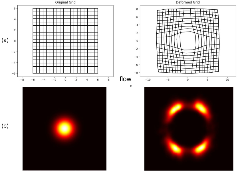
Figure 9 shows the effect of applying our DDNFflow to a regular grid and and a uni-modal Gaussian distribution.
B Posterior Approximation
We report the performance of other posterior estimation techniques than what we showed in Section 5.2. Other methods include Automatic Differentiation Variational Inference (ADVI) (Kucukelbir et al., 2017) and Householder flow (HF) (Tomczak and Welling, 2016)). For both of these methods, we used their implementation in the PyMC3 package (https://docs.pymc.io/). We repeat the experiment 10 times and the results of one instance is show in Figure 10. DDNFapproximates the true posterior(MCMC) accurately. Adding the scalar and drift transformations to the planar mapping improves the accuracy. The Table 2 reports the posterior mean of the two variables for MCMC, Plana + scalar + drift, and DDNF.
| m () | L | |
|---|---|---|
| MCMC | 1290.0 6.5 | 1560.9 65.0 |
| DDNF | 1289.7 25.1 | 1354.9 71.54 |
| planar-NF | 1600.0 594.7 | 1268.1 390.8 |
C Training Setup for the VAE Experiment
Network Architecture:
For the MNIST dataset, we implement the encoder of the VAE as an MLP with one hidden layer of size 128 and a latent code of dimension 40. The decoder is also an MLP with one hidden layer of size 128 that takes in an input of size 40 and outputs a vector of size 2828. The velocity fields in the DDNF are parameterized by two hidden layer with two hidden units each. We use tanh activation across all the hidden layers, and we use sigmoid activation on the output of the VAE network.
Training Details:
We train using SGD implemented in tensorflow. Across all experiments, we use a batch size of 100 and a learning rate of 0.001 and we train for 400 epochs. We report the minimum -ELBO on the test set for each of the methods averaged over three experiments with different random seeds (but common accross experiments).
Low Dimensional Latent Space:
We test our method on a lower dimensional latent space setting of the VAE where we use the same setup discussed in the previous sections, but with a latent code of dimension 2. Table 3 shows the results.
| Model | -ELBO |
|---|---|
| Vanilla VAE (diagonal covariance) | 149.43 0.14 |
| planar-NF [1] | 148.97 0.29 |
| NAF [2] | 144.10 0.50 |
| DDNF | 147.27 0.58 |
| DDNF + context | 143.68 0.51 |
D Deriving the Determinant of the Jacobian
where the first equality follows from the architecture of the ResNet cell in Figure 2-Top, the second equality is a results of , and the approximation is the second order Taylor expansion of around . We ignore polynomials terms of with the degree of three and higher.
E Other Choices of the Hilbert Norm
Several choices are possible of the Hilbert norm.
Identity and Laplacian operator
: Inspired by the research in the medical imaging community Beg et al. (2005a); Zhang and Fletcher (2015), we set where is an integer power and is the Laplacian operator with respect to . Since the Laplacian is a negative semidefinite operator, . The Laplacian encourages smoothness of the velocity field, i.e., non-smooth velocity field result in large Laplacian value.
There are several advantages of this choice of inner product. For sufficiently large powers, , the geodesic regularization guarantees existence of diffeomorphic flows, as long as the norm of the velocities are bounded. Without this condition, the flow of a differentiable velocity field is only guaranteed to exist over some unknown interval , not necessarily up to . This is due to the Picard-Lindelöf existence theorem for ODEs. However, as shown in Dupuis et al. (1998), we can guarantee that the flow of a velocity field, given by eq. 3, generates a diffeomorphism at time , if the space of velocity fields satisfy certain regularity conditions. This regularity condition is that the space of velocities, , be continuously embedded in the Sobolev space , i.e., the space of velocity fields with bounded generalized derivative.
Note that the Laplacian operator can be viewed as the trace of the Hessian matrix with respect to and the same trick applied in Eq. 8 can be used to efficiently compute the trace. Thanks to the reverse-mode differentiation introduced by Pearlmutter (1994), the Hessian-vector products can be computed efficiently in (). If , we retrieve the -norm. The simply shrinks the velocity toward zero. When the DDNF has few cells (i.e., is large), we found that even a simple regularization of helps the Taylor expansion in eq. 7 to be more accurate. In this paper, we set the because we use for non-linearity and our velocity field is smooth by construction.