Analytical Convergence Regions of Accelerated Gradient Descent in Nonconvex Optimization under Regularity Condition

This paper focuses on a special yet important case of nonconvex optimization, where the objective function $f(\cdot)$ satisfies the Regularity Condition (RC) [17], defined as follows.

It is straightforward to check that one must have $\mu\lambda\leq 1$ by Cauchy-Schwartz inequality. RC can be regarded as a combination of one-point strong convexity and smoothness [18], and does not require the function $f(\cdot)$ to be convex. RC has appeared in a wide range of applications, a partial list of which includes phase retrieval [17], deep linear neural networks [23], shallow nonlinear neural networks [24] and matrix sensing [25, 26].

Our framework can handle the general case where RC only holds locally as defined. To simplify the presentation, we will first assume RC holds globally, i.e. $\epsilon=\infty$ in Definition 1, in which case $x^{\star}$ becomes the global minimizer correspondingly. It turns out that our main results can be directly applied to the case when RC holds locally, using proper initializations, which will be explained in detail in Section 5. Without ambiguity, we will omit the neighborhood radius $\epsilon$ and use the notation $RC(\mu,\lambda)$ to denote the global RC in the derivation of the main results.

In practice, AGD methods are widely adopted for its ability to accelerate the convergence. Two widely-used acceleration schemes include Nesterov’s accelerated gradient (NAG) method [28], given as

where $\alpha>0$ is the step size, $0\leq\beta<1$ is the momentum parameter; and Heavy-Ball (HB) method [29], given as

where $\alpha>0$ is the step size, $0\leq\beta<1$ is the momentum parameter. In fact, we can describe a general AGD method that subsumes HB and NAG as special cases:

Despite the empirical success, the convergence of AGD in the nonconvex setting remains unclear to a large extent. For example, it is not known whether AGD converges under RC, whether it converges linearly if it does and how to set the step size and the momentum parameters to guarantee its convergence. These challenging questions motivate us to look for new tools to better understand AGD for nonconvex optimization.

Observe that a general AGD method (5) can be viewed as a linear dynamical system subject to nonlinear feedback:

To see this, let $z_{k}^{(1)}=z_{k}$, and $z_{k}^{(2)}=z_{k-1}$. Then it can be easily verified that (6) represents HB when $(\beta_{1},\beta_{2})=(\beta,0)$, and NAG when $(\beta_{1},\beta_{2})=(\beta,\beta)$.

Let $\otimes$ denote the Kronecker product. We use the notation $G(A,B,C,D)$ to denote a dynamical system $G$ governed by the following iterative state-space model:

where $I_{n}$ is the identity matrix of size $n$. If we define $\phi_{k}=\left[\begin{array}[]{c}z_{k}^{(1)}\\ z_{k}^{(2)}\end{array}\right]$ as the state, $u_{k}$ as the input and $y_{k}$ as the output, then (6) can be regarded as a dynamical system shown in Figure 1, where the feedback $\nabla f(y_{k})$ is a static nonlinearity that depends on the gradient of the loss function, and $G(A,B,C,D)$ is a linear system specified by

In the following, we will illustrate how to show the convergence of AGD. First, define $\phi_{*}=\left[\begin{array}[]{c}x^{\star}\\ x^{\star}\end{array}\right]$ as the equilibrium of the dynamical system (6). If the system is (globally) asymptotically stable, then $\phi_{k}\xrightarrow{k\rightarrow\infty}\phi_{*}$. It further implies $z_{k}\xrightarrow{k\rightarrow\infty}x^{\star}$. In other words, the asymptotic stability of the dynamical system can indicate the convergence of the iterates to a fixed point. From now on, we focus on the stability analysis of the feedback control system (6).

The stability analysis of the feedback control system (6) can be carried out using robust control theory. The main challenge is on the nonlinear feedback term $u_{k}=\nabla f(y_{k})$. Our key observation is that RC can be rewritten as the following quadratic constraint:

where $y_{*}=x^{\star}$ and $u_{*}=\nabla f(y_{*})=0$. Applying the quadratic constraint framework in [1], we can derive an LMI as a sufficient stability condition as stated in the following proposition. A formal proof of this result can be found in the appendix.

We first introduce the KYP lemma and the reader is referred to [30] for an elegant proof.

The general KYP lemma only asks $P$ to be symmetric instead of being positive definite (PD) as in our problem. To ensure that the KYP lemma can be applied to solve (9), some adjustments of the lemma are necessary. In fact, we observe that if $A$ of the dynamical system is Schur stable and the upper left corner of $M$, denoted as $M_{11}$, is positive semidefinite (PSD), then by checking the principal minor $M_{11}+A^{T}PA-P\prec 0$, we know $P$ satisfying (12) must be PD. We define these conditions on $A$ and $M$ as KYP Conditions, which are restrictions to make sure that all solutions of symmetric $P$ for (12) are PD.

Thus we can conclude the following corollary.

One can easily check, however, that $A$ and $M$ of a general AGD in (9) do not satisfy the KYPC($A,M$). Therefore, we need to rewrite the dynamical system (6) in a different way to satisfy the KYPC($A,M$), so that its stability analysis can be done by combining Proposition 1 and Corollary 1. In the following, we first introduce a way to rewrite the dynamical system to satisfy the KYPC($A,M$).

Recall that a general AGD can be written as (5). Here we introduce a slack variable $\delta$ to rewrite the algorithm:

Observe that for any value of $\delta$, (15) provides the same update rule as (5). It can be viewed as a generalized representation of the dynamical systems corresponding to the targeted AGD. Similar to (6), we rewrite (15) as a dynamical system $G(A^{\prime},B^{\prime},C^{\prime},D^{\prime})$:

Correspondingly,

In addition to the adjustment of the dynamics, the feedback of $G(A^{\prime},B^{\prime},C^{\prime},D^{\prime})$ also differs from that in (6). As a consequence, the quadratic bound for the new feedback $u_{k}=-\alpha\nabla f(y_{k})-\delta y_{k}$ is shifted as stated in the following lemma.

Now we have general representations of $A^{\prime}$, $M^{\prime}$ with one unknown parameter $\delta$. We need to certify the region of $(\alpha,\beta_{1},\beta_{2})$ such that its corresponding ($A^{\prime},M^{\prime}$) has at least one $\delta$ satisfying the KYPC($A^{\prime},M^{\prime}$).

By Lemma 3, if the parameters of a fixed AGD with $(\alpha,\beta_{1},\beta_{2})$ satisfy (18), then all feasible symmetric $P$’s for (14) can be guaranteed to be PD. Now we are ready to use the KYP lemma to complete the convergence analysis of an accelerated algorithm.

By Proposition 1, we can solve the stability of the new system (16) by finding some feasible $P\succ 0$ to the key LMI (9) with respect to the corresponding $(A^{\prime},B^{\prime},C^{\prime},D^{\prime},M^{\prime})$ for some rate $0<\rho<1$.

We are interested in obtaining the analytical region of $(\alpha,\beta_{1},\beta_{2})$ that guarantees the linear convergence of AGD under RC. We use the following strict matrix inequality without caring about a specific rate $\rho$,

Observe that now (19) is of the same form as (14). By the KYP lemma (Corollary 1), under KYPC($A^{\prime},M^{\prime}$) (19) can be equivalently solved by studying the following FDI:

By simplifying (20) we observe that all uncertain terms can be canceled out and then conclude the following lemma.

We omit the proof of Lemma 4 since it follows easily from Corollary 1 and some simple calculations to simplify (20).

By setting different $\beta_{1},\beta_{2}$ in (21), we can obtain the convergence condition of a general AGD method using the KYP lemma. In the following, we focus on the two most important cases: HB and NAG and other cases can be discussed in a similar way. The stability regions of HB and NAG can be obtained by letting $\beta_{2}=0$ and $\beta_{1}=\beta_{2}=\beta$ in (21), respectively. Then we can obtain Theorem 1 and Theorem 2.

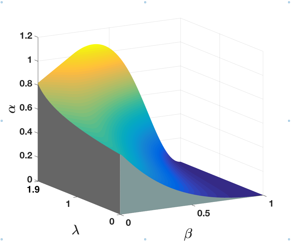
The analytical results stated in the above theorems can provide rich insights on the convergence behaviors of AGD. Take the convergence region of HB as an example. In Figure 2 (a), we fix the RC parameter $\lambda=0.5$ and vary $\mu$ within $[0.01,1.9]$, while in Figure 2 (b), we fix $\mu=0.5$ and vary the value of $\lambda$ within $[0.01,1.9]$. Observe that when we fix one of the RC parameter and increase the other, the stability region of ($\alpha,\beta$) gets larger.

Notice that $\mu$ plays a role similar to the inverse of the smoothness parameter, and therefore, it dominantly determines the step size, which is clearly demonstrated in Figure 2 (a). In addition, when we fix the values of a pair of ($\mu,\lambda$) (e.g. Figure 3), we can see that even when $\alpha$ exceeds the value of the bound of GD (the maximal feasible $\alpha$ when $\beta=0$), the Heavy-ball method can still ensure convergence when we choose $\beta$ properly. This property has not been discussed in the literature.

We emphasize that our theoretic analysis is a complement rather than a replacement for the numerical LMI approach in [1]. Our closed-form expressions for the stability region do provide some complementary benefits to the numerical approach in [1]. First, from our closed-form formulas, one can tell that the stability region of HB is well described by the feasible set of some relatively simple quadratic inequalities while the characterization of the stability region boundary of NAG partially involves a fourth-order polynomial. Such a difference is not directly reflected by the numerical LMI approach in [1]. Actually our closed-form expression for the stability region of HB is quite simple. Our study on HB and NAG just illustrates that the interpretability of the analytical formulas for the stability region depends on the specific momentum method being analyzed. Second, the stability region is easier and faster to visualize from analytical forms than numerical results. When given a pair of $(\mu,\lambda)$, one needs to make a small grid of $(\alpha,\beta_{1},\beta_{2})$ and solve an LMI for each single pair, which is computationally complex but can be avoided if we have closed-form analytical results. More importantly, the LMI conditions in Lessard et al. [16] can only certify convergence numerically for fixed $(\alpha,\beta_{1},\beta_{2})$ under a given pair of RC parameter $(\mu,\lambda)$. However, our analytical results provide continuous stability regions with respect to $(\mu,\lambda)$, which is hard to achieve using numerical results.

In this subsection, we will use a simple example satisfying RC globally to show show how our results help to choose parameters of different first-order methods in practice.

Consider a loss function as shown in Figure 4(a) with an expression as

This nonconvex loss function was also discussed in [19, 18]. One can check that $f$ satisfies $RC(0.5,0.5)$.

We initialize at $x_{0}=x_{1}=24$ and choose $\alpha=0.1$. By Theorem 1, HB can converge when $\beta<0.5942$. For NAG, we choose $\beta<0.6950$ according to Theorem 2. Furthermore, it is common to choose the hyper-parameter $\beta$ as large as possible to obtain a better performance. Therefore, the corresponding $\beta$’s to HB and NAG are chosen as $0.59$ and $0.69$, respectively. In Figure 4(b), we see that all the three algorithms can converge and the two accelerated methods HB and NAG obviously outperform GD.

References

- [1] L. Lessard, B. Recht, and A. Packard, “Analysis and design of optimization algorithms via integral quadratic constraints,” SIAM Journal on Optimization, vol. 26, no. 1, pp. 57–95, 2016.
- [2] B. Hu and L. Lessard, “Dissipativity theory for Nesterov’s accelerated method,” in Proceedings of the 34th International Conference on Machine Learning, vol. 70, 2017, pp. 1549–1557.
- [3] B. Hu, P. Seiler, and A. Rantzer, “A unified analysis of stochastic optimization methods using jump system theory and quadratic constraints,” in Proceedings of the 2017 Conference on Learning Theory (COLT), vol. 65, 2017, pp. 1157–1189.
- [4] B. Hu, S. Wright, and L. Lessard, “Dissipativity theory for accelerating stochastic variance reduction: A unified analysis of SVRG and Katyusha using semidefinite programs,” in Proceedings of the 35th International Conference on Machine Learning, vol. 80, 2018, pp. 2038–2047.
- [5] M. Fazlyab, A. Ribeiro, M. Morari, and V. M. Preciado, “Analysis of optimization algorithms via integral quadratic constraints: Nonstrongly convex problems,” SIAM Journal on Optimization, vol. 28, no. 3, pp. 2654–2689, 2018.
- [6] A. C. Wilson, B. Recht, and M. I. Jordan, “A lyapunov analysis of momentum methods in optimization,” arXiv preprint arXiv:1611.02635, 2016.
- [7] R. Nishihara, L. Lessard, B. Recht, A. Packard, and M. I. Jordan, “A general analysis of the convergence of admm,” in Proceedings of the 32nd International Conference on International Conference on Machine Learning, vol. 37, 2015, pp. 343–352.
- [8] A. Sundararajan, B. Hu, and L. Lessard, “Robust convergence analysis of distributed optimization algorithms,” in 2017 55th Annual Allerton Conference on Communication, Control, and Computing (Allerton). IEEE, 2017, pp. 1206–1212.
- [9] A. Cherukuri, E. Mallada, S. Low, and J. Cortés, “The role of convexity in saddle-point dynamics: Lyapunov function and robustness,” IEEE Transactions on Automatic Control, vol. 63, no. 8, pp. 2449–2464, 2017.
- [10] B. Hu, P. Seiler, and L. Lessard, “Analysis of approximate stochastic gradient using quadratic constraints and sequential semidefinite programs,” arXiv preprint arXiv:1711.00987, 2017.
- [11] B. Hu and L. Lessard, “Control interpretations for first-order optimization methods,” in 2017 American Control Conference (ACC). IEEE, 2017, pp. 3114–3119.
- [12] B. Van Scoy, R. A. Freeman, and K. M. Lynch, “The fastest known globally convergent first-order method for minimizing strongly convex functions,” IEEE Control Systems Letters, vol. 2, no. 1, pp. 49–54, 2018.
- [13] S. Cyrus, B. Hu, B. Van Scoy, and L. Lessard, “A robust accelerated optimization algorithm for strongly convex functions,” in 2018 Annual American Control Conference (ACC). IEEE, 2018, pp. 1376–1381.
- [14] N. K. Dhingra, S. Z. Khong, and M. R. Jovanovic, “The proximal augmented lagrangian method for nonsmooth composite optimization,” IEEE Transactions on Automatic Control, vol. 64, no. 7, pp. 2861 – 2868, 2019.
- [15] A. S. Kolarijani, P. M. Esfahani, and T. Keviczky, “Fast gradient-based methods with exponential rate: A hybrid control framework,” in Proceedings of the 35th International Conference on Machine Learning, vol. 80, 2018, pp. 2728–2736.
- [16] N. S. Aybat, A. Fallah, M. Gurbuzbalaban, and A. Ozdaglar, “Robust accelerated gradient methods for smooth strongly convex functions,” arXiv preprint arXiv:1805.10579, 2018.
- [17] E. J. Candes, X. Li, and M. Soltanolkotabi, “Phase retrieval via wirtinger flow: Theory and algorithms,” IEEE Transactions on Information Theory, vol. 61, no. 4, pp. 1985–2007, 2015.
- [18] Y. Chi, Y. M. Lu, and Y. Chen, “Nonconvex optimization meets low-rank matrix factorization: An overview,” IEEE Transactions on Signal Processing, vol. 67, no. 20, pp. 5239–5269, 2019.
- [19] Y. Chen and E. J. Candès, “Solving random quadratic systems of equations is nearly as easy as solving linear systems,” Communications on Pure and Applied Mathematics, vol. 70, no. 5, pp. 822–883, 2017. [Online]. Available: http://dx.doi.org/10.1002/cpa.21638
- [20] H. Zhang, Y. Liang, and Y. Chi, “A nonconvex approach for phase retrieval: Reshaped wirtinger flow and incremental algorithms,” Journal of Machine Learning Research, vol. 18, no. 141, pp. 1–35, 2017.
- [21] H. Zhang, Y. Chi, and Y. Liang, “Provable non-convex phase retrieval with outliers: Median truncated Wirtinger flow,” in International Conference on Machine Learning, 2016, pp. 1022–1031.
- [22] G. Wang, G. B. Giannakis, and Y. C. Eldar, “Solving systems of random quadratic equations via truncated amplitude flow,” IEEE Transactions on Information Theory, vol. 64, no. 2, pp. 773–794, 2017.
- [23] Y. Zhou and Y. Liang, “Characterization of gradient dominance and regularity conditions for neural networks,” arXiv preprint arXiv:1710.06910, 2017.
- [24] Y. Li and Y. Yuan, “Convergence analysis of two-layer neural networks with ReLU activation,” in Advances in Neural Information Processing Systems, 2017, pp. 597–607.
- [25] S. Tu, R. Boczar, M. Simchowitz, M. Soltanolkotabi, and B. Recht, “Low-rank solutions of linear matrix equations via procrustes flow,” in International Conference on Machine Learning, 2016, pp. 964–973.
- [26] Y. Li, Y. Chi, H. Zhang, and Y. Liang, “Non-convex low-rank matrix recovery with arbitrary outliers via median-truncated gradient descent,” Information and Inference: A Journal of the IMA, 2019. [Online]. Available: https://doi.org/10.1093/imaiai/iaz009
- [27] E. J. R. Pauwels, A. Beck, Y. C. Eldar, and S. Sabach, “On fienup methods for sparse phase retrieval,” IEEE Transactions on Signal Processing, vol. 66, no. 4, pp. 982–991, 2017.
- [28] Y. Nesterov, Introductory Lectures on Convex Optimization: A Basic Course. Springer Science & Business Media, 2003, vol. 87.
- [29] B. T. Polyak, “Some methods of speeding up the convergence of iteration methods,” USSR Computational Mathematics and Mathematical Physics, vol. 4, no. 5, pp. 1–17, 1964.
- [30] A. Rantzer, “On the kalman-yakubovich-popov lemma,” Systems & control letters, vol. 28, no. 1, pp. 7–10, 1996.
- [31] R. H. Keshavan, A. Montanari, and S. Oh, “Matrix completion from a few entries,” IEEE transactions on information theory, vol. 56, no. 6, pp. 2980–2998, 2010.