Universality and scaling in multi-field $\alpha$-attractor preheating

We start by analyzing the background motion of the $\phi$ and $\chi$ fields, in order to identify the regime of effectively single-field motion and describe CMB constraints on the model parameters. We initially assume that $\chi(t)=0$ at background level, which is indeed a dynamical attractor, as we will show later. Eq. (6) in the slow-roll approximation and for $\tilde{\phi}/\sqrt{\tilde{\alpha}}\gg 1$, which holds during inflation, becomes

where $H/\mu\simeq\sqrt{\tilde{\alpha}/3}$, leading to

The slow-roll parameters become

The end of inflation defined as $\epsilon=1$, based on the slow-roll analysis, occurs at

The last term in Eq. (13) is subdominant for small $\tilde{\alpha}$ and can be safely ignored, leading to ${\tilde{\phi}_{\rm end}/\sqrt{\tilde{\alpha}}}\simeq{0.6(1.7+2\log n)}$. Even though the slow-roll approximation fails near the end of inflation, the scaling $\tilde{\phi}_{\rm end}/\sqrt{\tilde{\alpha}}={\cal O}(1)$ is valid over the whole range of potential parameters $\alpha$ and $n$ that we considered, as shown in Fig. 1. The Hubble scale at $\epsilon=1$ is

where the numerical factor in the last equality of Eq. (14) is fitted from the bottom right panel of Fig. 1.

The tensor-to-scalar ratio for single-field motion is

In general $r=\alpha\times{\cal O}(10^{-3})$ for modes that exit the horizon at $N\sim 55$ $e$-folds before the end of inflation. The dimensionless power spectrum of the (scalar) density perturbations is measured to be

Using the expression for the scalar power spectrum from single field slow-roll inflation

and the value of the Hubble scale at the plateau of the potential $H^{2}\simeq\tilde{\alpha}\mu^{2}/3$, it is straightforward to see that $\mu\sim 10^{-5}M_{\rm Pl}$. Hence the scale of $\mu$ fixes the amplitude of the scalar power spectrum, independent of $\alpha$ and $n$. By using $\mu$ to re-scale time, it is trivial to connect the preheating calculations performed in the present work to observational constraints on the potential parameters.

It can be easily seen that the potential of Eq. (3) exhibits a minimum at $\chi=0$ for all values of $\phi$. However, the approach to this potential “valley” is important and could in principle leave observational signatures, if it occurs close to the time at which the CMB-relevant scales leave the horizon.

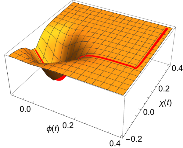
Fig. 2 shows the transition to the single-field trajectory for $n=3/2$ and $\alpha=0.001$. The initial conditions are $\phi_{0}=\chi_{0}$, chosen such that there would be $60$ $e$-folds of inflation for $\chi_{0}=0$. We see two distinct stages of inflation: initially $\phi(t)$ remains almost constant and $\chi(t)$ follows a slow-roll motion until it reaches the minimum $\chi=0$. Then, after a sharp turn in field-space, the field $\phi(t)$ follows a slow-roll motion towards the global minimum of the potential, while $\chi$ stays exponentially close to zero. Hence to a good approximation, the whole inflationary era is separated into two sequential periods of distinct single-field motion.

Starting from a wide range of initial conditions $\phi_{0}\equiv\phi(0)$ and $\chi_{0}\equiv\chi(0)$, we see that the system generically follows the two-stage evolution shown in Fig. 2, proceeding along $\chi(t)=0$ during the last stage of inflation and during the post-inflationary oscillations. Figure 3 shows the transition to the single-field motion along $\chi=0$ for broad conditions, constrained to provide more than $60$ $e$-folds of inflation. Beyond the fact that the single field trajectory along $\chi(t)=0$ is a dynamical attractor for the generalized two-field T-model, its predictions are robust with respect to $\chi_{0}$. As shown in Fig. 3, the number of $e$-folds along the second stage $\chi(t)=0$ is much larger than the number of $e$-folds along the first stage $\phi(t)={\rm const}$. The range of values $\{\phi_{0},\chi_{0}\}$ that place the turn-rate spike (the transition between the two single-field motions) at the observable window $50\lesssim N_{*}\lesssim 60$ is very narrow, requiring delicate fine-tuning. Hence the generic observational prediction of these models for the CMB is that of usual single-field $\alpha$-attractors. This behavior can be understood analytically. Considering the number of $e$-folds along a single-field trajectory we get

As a quick estimate of the number of $e$-folds we can use $\Delta N_{1}\sim(H/|\dot{\chi}|)\Delta\chi\sim(H/|\dot{\chi}|)\chi_{0}$ during the first stage and $\Delta N_{2}\sim(H/|\dot{\phi}|)\Delta\phi\sim(H/|\dot{\phi}|)\phi_{0}$ during the second stage of inflation. Assuming that the Hubble scale does not change much during inflation

Fig. 4 shows the ratio $|\dot{\phi}/\dot{\chi}|$ as a function of $\phi$ for several values of $\chi_{0}$. We see that for large values of $\phi_{0}$, required to give a sufficient number of $e$-folds of inflation, $|\dot{\chi}|={\cal O}(10)|\dot{\phi}|$, hence $N_{1}={\cal O}(0.1)N_{2}$ for typical values of $\{\phi_{0},\chi_{0}\}$. While there is potentially interesting phenomenology from the turning trajectories, it is absent for generically chosen initial conditions. Since we are only interested in the preheating behavior of the two-field T-model, we will not pursue this subject further here.

A novel phenomenon that manifests itself in scalar field systems on a negatively curved manifold is “geometrical destabilization” [31], where the presence of a negative field-space Ricci term can turn a stable direction into an unstable one. The study of the effective mass for the $\phi$ and $\chi$ fluctuations will be performed in Section III. In order to check the stability of the single-field trajectory, it suffices to use the effective super-horizon isocurvature mass

During inflation and using the slow-roll conditions, we get

which is positive. However, close to the end of inflation the slow-roll approximation fails and the result cannot be trusted. Hence the model under study is safe against geometrical destabilization effects during inflation. The effective mass of isocurvature fluctuations can become negative after the end of inflation, but this falls under the scope of tachyonic preheating, as will be discussed in Section III. Figure 5 shows the isocurvature effective mass-squared during the last $e$-folds of inflation, showing that it is indeed positive until very close to the end, hence no Geometrical Destabilization will occur³³ 3 Recently Ref. [35] showed the existence of yet another possible evolution for $\alpha$-attractor models, angular inflation, where the background motion proceeds along the boundary of the Poincare disk. We did not see this behavior arise in the context of the two-field T-model studied here, even for highly curved manifolds.. However Fig. 5 shows that all computations, either using linear analysis as the ones performed here, or full lattice simulations like in Ref. [75], must be initialized more than an $e$-fold before the end of inflation, where the effective isocurvature mass-squared is positive and the connection to the Bunch Davies vacuum is possible.

In order to study the post-inflationary background evolution of the inflaton field $\phi(t)$, it is convenient to work in terms of the rescaled field variable ${\delta\equiv\tilde{\phi}/\sqrt{\tilde{\alpha}}}$ and re-write the equation of motion for the inflaton field $\phi$ as

where

The field re-scaling leads to $\delta={\cal O}(1)$ at the end of inflation and during preheating. We see that the evolution of $\delta$, if one neglects the Hubble drag term, does not depend on $\alpha$. This is reminiscent of non-minimally coupled models of inflation, where the background equation of motion approaches one “master equation”, when properly normalized, and thus the background motion is self-similar for large values of the non-minimal coupling $\xi$. In reality the background evolution has a mild dependence on $\alpha$, arising from the (very weak) dependence of $\delta_{\rm end}$ on $\alpha$, which is shown in Fig. 1. Fig. 6 shows the period of background oscillations, if we neglect the Hubble drag and initialize the oscillation at $\delta_{\rm init}=\phi_{\rm end}/\sqrt{\alpha}$. We see that the period $T\sim 10$. More importantly, there is a significant separation of scales between the background oscillation frequency $\omega=2\pi/T$ and the Hubble scale. The relation can be roughly fitted as $\omega/H_{\rm end}\sim 1/\sqrt{\tilde{\alpha}}$. This shows that there are more background oscillations per Hubble time (or per $e$-fold) for smaller values of $\tilde{\alpha}$, hence for highly curved field-space manifolds.

The covariant formalism that must be used to study the evolution of fluctuations in models comprised of multiple scalar fields on a curved manifold has been developed and presented in Refs. [77, 28], described in detail in Ref. [78] and extensively used in Refs. [79, 80, 81] for studying preheating in multi-field inflation with non-minimal couplings to gravity. The gauge-invariant perturbations obey

where the mass-squared matrix is given by

and ${\cal R}^{I}_{\>LMJ}$ is the Riemann tensor constructed from ${\cal G}_{IJ}(\varphi^{K})$. For the model at hand, where the background motion is restricted along the $\chi=0$ direction, the field-space structure simplifies significantly ${\cal G}_{IJ}(\chi=0)=\delta_{IJ}$ and $\Gamma^{I}_{JK}=0$, hence all covariant derivatives become partial derivatives and the quantization of the fluctuations proceeds as usual. This is not the case for other parametrizations of the field-space, or other background trajectories, where ${\cal G}_{IJ}\neq\delta_{IJ}$, and one would have to use the field-space vielbeins to properly quantize the system, as done for example in Ref. [78].

We rescale the perturbations as $Q^{I}(x^{\mu})\rightarrow X^{I}(x^{\mu})/a(t)$ and work in terms of conformal time, $d\eta=dt/a(t)$. This allows us to write the quadratic action in a form that resembles Minkowski space, which makes their quantization straightforward. The quadratic action becomes

where

and $R$ is the space-time Ricci scalar. The energy density of the two fields in momentum-space becomes

where we used the equation of motion for the second equality and defined the effective frequency-squared as

We promote the fields $X^{I}$ to operators $\hat{X}^{I}$ and expand $\hat{X}^{\phi}$ and $\hat{X}^{\chi}$ in sets of creation and annihilation operators and associated mode functions

and we define $u^{\phi}\equiv v$ and $u^{\chi}\equiv z$. Since the modes decouple on a single-field background with vanishing turn-rate, the equations of motion are

The effective masses of the two types of fluctuations, along the background motion and perpendicular to it, consist of four distinct contributions [78]:

with

The various component of the effective mass-squared arises from a different source:

• •

  $m_{1,I}^{2}$ is the usual effective mass term derived from the curvature of the potential around the minimum.

• •

  $m_{2,I}^{2}$ comes from the geometry of field-space and has no analogue in models with a trivial field space.

• •

  $m_{3,I}^{2}$ arises due to the presence of coupled metric perturbations by considering linear fluctuations in the metric as well as in the fields. This contribution vanishes in the limit of infinitely rigid space-time.

• •

  $m_{4,I}^{2}$ encodes the curvature of space-time.

In general $m_{3,\chi}^{2}=0=m_{2,\phi}^{2}$, since the coupled metric fluctuations described by $m_{3,I}^{2}$ only affect the adiabatic modes $\delta\phi$, while the field-space curvature described by $m_{2,I}^{2}$ only affects the isocurvature modes⁴⁴ 4 The terms “adiabatic” and “isocurvature” refer to fluctuations along and perpendicular to the background trajectory respectively. $\delta\chi$. In our case, both $m_{3,I}^{2}$ and $m_{4,I}^{2}$ are subdominant for highly curved field spaces $\tilde{\alpha}\ll 1$, as can be seen from the various scalings of the terms in Eq. (32)

The small value of $m_{4,I}^{2}$ is one further indication that fluctuations behave almost as if they were in flat spacetime. These scalings agree very well with numerical evaluations for a large range of $\tilde{\alpha}$, as shown in Fig. 7.

A closer analysis of scaling relations for $m_{{\rm eff},\chi}^{2}$, will be performed in Section III.2. Meanwhile, within the single-field attractor along $\chi=0$, the energy densities for adiabatic and isocurvature perturbations take the simple form [78]

where we thus approximate the two effective masses as

where ${\cal R}=-4/3\alpha$ is the field space Ricci curvature scalar and we dropped the subdominant terms. We must keep in mind that $Q^{\phi}\sim v_{k}/a(t)$ and $Q^{\chi}\sim z_{k}/a(t)$. We measure particle production with respect to the instantaneous adiabatic vacuum [53]. The initial conditions for preheating can be read off from Eq. (31), using the WKB approximation and starting during inflation, when the effective mass is positive

In the far past $a(\eta)\to 0$, hence $\{\omega_{\phi}(k,\eta),\omega_{\chi}(k,\eta)\}\to k$, which makes the solutions of Eqs. (38) and (39) match to the Bunch-Davies vacuum during inflation.

Since we will be performing the computations in cosmic time, we write the equations of motion for the two types of fluctuations. The fluctuation equation for the $\phi$ field (adiabatic direction) is

where we neglected the term arising from the coupled metric fluctuations, that is proportional to $M_{\rm Pl}^{-2}$. We again rescale time by $\mu$ giving us

where the potential-dependent term of the effective frequency is

The results for the isocurvature modes $\delta\chi$ or $Q_{\chi}$ are similar

The last term in the above equation is the Riemann contribution to the effective mass-squared $\omega^{2}_{\chi}$

Since the self-resonance of $\delta\phi$ modes in these models has been extensively studied (see for example Ref. [82]), we will focus our attention on $\delta\chi$ fluctuations, which can undergo tachyonic excitation, which is generally more efficient than parametric amplification. Also the excitation of $\delta\chi$ modes is a truly multi-field phenomenon that depends crucially on the field-space geometry.

We examine in detail the effective frequency-squared for the $\delta\chi$ fluctuations, $\omega_{\chi}^{2}(k,t)$. For simplicity we will focus on the case of $n=3/2$, which matches the potential used in the lattice simulations presented in Ref. [75]. The generalization of our results for other potentials is discussed in Section IV.

In the top left panel of Fig. 8 we see the evolution of the background field $\phi(t)$, rescaled as $\delta(t)=\phi(t)/\sqrt{\alpha}$ after the end of inflation and we take $t=0$ as the end of inflation. We see that inflation ends at $\phi(t)/\sqrt{\alpha}\simeq 3$ for all three cases considered here, consistent with Fig. 1. The main difference is both the frequency of oscillation and the decay of the amplitude of the background for different values of $\alpha$.

The maximum tachyonically excited wavenumber for the various cases under consideration is $k_{\rm max}\simeq 0.87\mu$ for $\tilde{\alpha}=10^{-2}$, $k_{\rm max}\simeq 1.04\mu$ for $\tilde{\alpha}=10^{-3}$ and $k_{\rm max}\simeq 1.11\mu$ for $\tilde{\alpha}=10^{-4}$. So we can say⁵⁵ 5 In the units of Appendix C and Ref. [75], this corresponds to $k_{\rm max}\simeq{1\over\sqrt{\alpha}}M^{2}/M_{\rm Pl}$, leading to $k_{\rm max}\simeq 33M^{2}/M_{\rm Pl}$ for $\alpha=10^{-3}$ and $k_{\rm max}\simeq 100M^{2}/M_{\rm Pl}$ for $\alpha=10^{-4}$. This is consistent with Figure 5 of Ref. [75]. that $k_{\rm max}\simeq\mu$ for all values of $\tilde{\alpha}\ll 1$. Furthermore, we see that background motion corresponding to larger values of $\tilde{\alpha}$ shows greater damping. This is consistent with the observation that $H_{\rm end}\sim\sqrt{\tilde{\alpha}}$, hence the Hubble damping term is smaller for highly curved field-space manifolds.

Examining the tachyonic contribution to $\omega^{2}_{\chi}(k)$, a very simple scaling emerges

This is again consistent with Fig. 8, especially as the value of $\tilde{\alpha}$ gets smaller.

Since the tachyonic contribution to the effective mass-squared is similar for models with different values of $\tilde{\alpha}$, the tachyonic amplification of the relevant mode-functions after each oscillation will be also similar. Fig. 9 shows the evolution of $\omega^{2}_{\rm min}$ and $k_{\rm max}$ for each subsequent tachyonic region. It is worth emphasizing that $\omega^{2}_{\rm min}$ is determined solely by the corresponding minimum (maximum negative) value of $m_{2,\chi}^{2}$. The maximum negative value of $m_{2,\chi}^{2}$ occurs when $|\dot{\phi}|$ is maximized, or equivalently when $\phi=0$. At this point, the potential can be Taylor-expanded as

For $n>1$ the effective mass component vanishes for $\chi=0$. In particular for $n=3/2$ the effective mass component becomes $\partial^{2}_{\chi}V(\phi=0,\chi)\sim|\chi|$, as shown in Fig. 8. The case of $n=1$ is different and we consider it in Section IV. We see that both the maximum (negative) contribution of $m_{2,\chi}^{2}$, as well as the range of tachyonically excited wavenumbers decrease faster for larger values of $\tilde{\alpha}$, or less curved field-space manifolds. This can be traced back to the dependence of the Hubble scale on the field-space curvature, which scales as $H\propto\sqrt{\tilde{\alpha}}$. Hence in the first $e$-fold, or within the first Hubble-time after inflation, lower values of $\tilde{\alpha}$ will result in a larger number of tachyonic bursts and hence a larger overall amplification. Furthermore, a larger Hubble term for larger values of $\tilde{\alpha}$ will result in a faster red-shifting of the background field amplitude $\delta(t)$, resulting in a faster suppression of the parametric resonance, in line with Fig. 8.

We use the WKB analysis as described in Ref. [83], in order to make analytical progress in computing the amplification of the $\delta\chi$ modes during tachyonic preheating. In contrast to Refs. [84, 85, 86], where tachyonic preheating lasted for a few inflaton oscillations at most, in the present case, multiple inflaton oscillations might be required, in order to siphon enough energy from the inflaton into radiation modes. However, given the fact that the Hubble time is much larger than the period of oscillations, preheating will still be almost instantaneous in terms of the number of $e$-folds. Based on $\omega/H_{\rm end}\sim 1/\sqrt{\tilde{\alpha}}$, we can estimate the number of background oscillations occurring during the first $e$-fold of preheating to be $N_{\rm osc.}\sim 0.2/\sqrt{\tilde{\alpha}}$.

We neglect the effect of the expansion of the Universe, hence taking $H=0$. This is an increasingly good approximation for smaller values of $\tilde{\alpha}$, since $H_{\rm end}\sim\sqrt{\tilde{\alpha}}$. Furthermore, the static universe WKB analysis will provide a useful comparison to the Floquet analysis of Section III.4. The equation of motion for the fluctuations in the $\chi$ field becomes⁶⁶ 6 For the remainder of this work we denote the fluctuations of the $\chi$ field as $\chi_{k}$ rather than $\delta\chi_{k}$ for notational simplicity.

where

where the components of the effective mass are given in Eq. (33). Following Ref. [83], we write the WKB form of the mode-functions before, during and after a tachyonic transition (regions I, II and III respectively).

where $\Omega_{k}^{2}(t)=-\omega_{k}^{2}(t)$. The amplification factor after the first tachyonic region for each mode $k$ is

where $t_{\pm}$ are the points at which the effective frequency vanishes, $\omega_{k}^{2}(t_{\pm})=\Omega_{k}^{2}(t_{\pm})=0$.

Fig. 10 shows the result of the numerical solution and the WKB result before, during and after the first tachyonic amplification phase. We see that the agreement is very good, hence we can use the expression of Eq. (50) to estimate the growth rate of fluctuations.

As shown in Eq. (49), following the first tachyonic burst all modes with wavenumbers $k\leq k_{\rm max}$ will be amplified. Subsequent background oscillations will cause destructive or constructive interference, leading to the formation of stability and instability bands, the latter exhibiting no exponential growth. In Ref. [83] it is shown that the amplitude of the wavefunction for a mode with wavenumber $k$ after the $j$’th tachyonic burst is

where $\Theta_{k}$ is the total phase accumulated between two consecutive tachyonic regimes. We can define an averaged growth rate as

where $P(t)$ is a bounded (periodic) function and $\mu_{k}$ is the Floquet exponent, as we discuss in detail in Section III.4. Since there are two tachyonic regimes for each background oscillation, the Floquet exponent $\mu_{k}$ is extracted from Eq. (51) as

where $T$ is the background period of oscillation. As shown in Fig. 11, the Floquet exponent extracted from Eqs. (51) and (53) depends on time, albeit mildly after the first few tachyonic bursts. However, there is a clear asymptotic regime that emerges after the background inflaton field has undergone multiple oscillations. The asymptotic value should be compared to the “true” Floquet exponent, which we compute in Section III.4.

Floquet theory is a powerful tool for studying parametric resonance in the static universe approximation. The algorithm for computing Floquet charts can be found in the literature (see for example Ref. [53]).

We may further understand properties of the Floquet charts by examining the Fourier structure of certain field-space quantities. In the rigid-spacetime limit, Eq. (47) for the isocurvature modes $\chi_{k}$ may be written in the suggestive form

again using $m_{\rm eff,\chi}^{2}=m_{1,\chi}^{2}+m_{2,\chi}^{2}$ in the rigid-spacetime limit. This equation is of the form

where ${\cal P}(t)$ is a periodic matrix. The period of the background is $T$, but the period of $m^{2}_{{\rm eff},\chi}$ is $T/2$, since it depends quadratically on the background field $\phi(t+T)=\phi(t)$ and its derivative $\dot{\phi}(t+T)=\dot{\phi}(t)$. In Ref. [79] a semi-analytic method was described for computing the edges of the instability bands at arbitrary high accuracy, by reducing the system to an algebraic matrix equation. The truncation of the resulting matrices determines the number of Floquet bands that can be accurately computed. In the present work we determine the edges of the instability bands after the computation of the full Floquet chart using Mathematica.

Fig. 12 shows the Floquet charts for $n=3/2$ and $\tilde{\alpha}=10^{-2},10^{-3},10^{-4}$. We can see that, when normalized appropriately with $\tilde{\alpha}$, the Floquet charts look similar, especially when it comes to the first two instability bands, which essentially control the entirety of the parametric resonance. The relation between Floquet charts for different values of $\alpha$ becomes even more evident, when we show a few contours of the first instability bands on the same plot. It is then obvious that for $\tilde{\alpha}\lesssim 10^{-3}$ the parametric resonance in the static universe approximation is identical, regardless of the exact value of the field-space curvature⁷⁷ 7 For $\tilde{\alpha}=10^{-2}$ the edges of the first two instability bands follow the ones exhibited by $\tilde{\alpha}\ll 1$, while the low-$k$ edge of the first band shows slightly larger Floquet exponents.. This is no surprise, since the WKB analysis of Section III.3 predicted the scaling behavior of the parametric resonance strength for low values of $\tilde{\alpha}$. The Floquet chart of Fig. 12 can be considered a “master diagram”, from which the Floquet chart for arbitrary values of $\tilde{\alpha}\lesssim 0.01$ can be easily read-off by using the appropriate scaling with $\tilde{\alpha}$.

Finally, Fig. 13 shows the comparison between the Floquet exponent computed using the algorithm described in Ref. [53] and using the WKB analysis. We see that the WKB analysis is able to capture the existence of the first two instability bands, even though the shape does not perfectly match the fully numerical solution.

There are two complications introduced by studying preheating in an expanding universe: the (slow) decay of the amplitude of the background oscillations due to the non-zero Hubble drag and the red-shifting of the physical wavenumber $k_{\rm phys}=k_{\rm comoving}/a$ due to the increasing scale-factor $a(t)$. Both effects are comparable, so they must be studied together. While a WKB analysis can be performed in an expanding universe [83], it must take into account the evolution of both $k_{\rm phys}$ and $\phi(t)$ numerically. Since we believe that it will not add significantly to building intuition on the model at hand, we will not pursue it here. Instead we numerically solve the equations of motion for the $\chi$ fluctuations, working in the linear regime as follows: The evolution for the background inflaton field and the Hubble rate are solved numerically using Eqs. (22) and (23). We subsequently compute the produced $\chi$ fluctuations driven by the background inflaton field. The back-reaction of the produced $\chi$ fluctuations on the inflaton field or the Hubble rate is ignored. This is a valid approximation until the energy density of the $\chi$ fluctuations becomes comparable to the background inflaton energy density. We briefly discuss back-reaction effects in Appendix D. We start our computations several $e$-folds before the end of inflation, in order for the effective mass to be positive for all modes, according to Fig. 5 and so that the WKB solutions of Eq. (39) provide accurate initial conditions for our code.

Fig. 14 shows the spectra of the fluctuations in the $\chi$ field at different times. We see that the band structure of the static universe Floquet charts of Section III.4 has disappeared, essentially leaving behind a region of excited modes with comoving wavenumbers that satisfy $k\leq k_{\rm max}\approx\mu$. This occurs because each mode with a specific wavenumber $k$ redshifts through the bands of Fig. 12, hence a mode with $k\leq k_{\rm max}$ will eventually redshift into the main instability band. Even though the exact band structure is erased, the WKB analysis can still capture very well the behavior after the first tachyonic burst. We see that the amplification factor computed in Eq. (50) matches very well with the actual amplification. For small values of $\tilde{\alpha}$, where the Hubble scale is much smaller than the frequency of background oscillations, Eq. (50) can provide useful intuition for the behavior of the $\chi$ fluctuations during the first few $\phi$ oscillations. Using Eq. (14) the maximum excited wavenumber can be immediately compared to the Hubble scale at the end of inflation to give

Hence tachyonic amplification occurs predominately for sub-horizon modes, meaning that they will behave like radiation after the end of preheating.

Fig. 15 shows the evolution of the energy density in the background inflaton field $\phi$ and the fluctuations of the $\chi$ field. Considering a finite amount of wavenumbers $k<k_{\rm UV}$ initialized at the Bunch Davies vacuum, we can compute their energy density at the end of inflation to be

This corresponds to the red-dashed line of Fig. 15, where we took $k_{\rm UV}=1.5\mu$. This is not a physical energy density, since these are vacuum modes. It is however useful as a check of our numerical calculation. Using different values of $k_{\rm UV}$ leads to different early time behavior, as shown from the green-dashed line in Fig. 15. As long as $k_{\rm UV}\geq k_{\rm max}$, the exact choice of $k_{\rm UV}$ becomes irrelevant once tachyonic resonance begins and all modes within $k<k_{\rm max}$ become exponentially amplified. Hence the blue and green-dashed curves of Fig. 15, corresponding to $k_{\rm UV}=1.5\mu$ and $k_{\rm UV}=\mu$ respectively, become indistinguishable shortly after the end of inflation. In is interesting to note that we find for $n=3/2$ and $\alpha=10^{-4}$ that preheating will conclude at $N_{\rm reh}=0.2$, where the energy density in $\chi$ fluctuations equals the energy density in the background field. This result agrees well with the findings of Fig. 4 of Ref. [75], where the results of a full lattice code are shown for the same model parameters.

References

- [1] A. H. Guth, “The Inflationary Universe: A Possible Solution to the Horizon and Flatness Problems,” Phys. Rev. D 23 (1981) 347. doi:10.1103/PhysRevD.23.347
- [2] A. D. Linde, “A New Inflationary Universe Scenario: A Possible Solution of the Horizon, Flatness, Homogeneity, Isotropy and Primordial Monopole Problems,” Phys. Lett. 108B, 389 (1982). doi:10.1016/0370-2693(82)91219-9
- [3] Y. Akrami et al. [Planck Collaboration], “Planck 2018 results. X. Constraints on inflation,” arXiv:1807.06211 [astro-ph.CO].
- [4] A. A. Starobinsky, “A New Type of Isotropic Cosmological Models Without Singularity,” Phys. Lett. B 91, 99 (1980) [Phys. Lett. 91B, 99 (1980)].
- [5] D. I. Kaiser and E. I. Sfakianakis, “Multifield inflation after Planck: The case for nonminimal couplings,” Phys. Rev. Lett. 112 (2014): 011302, arXiv:1304.0363 [astro-ph.CO].
- [6] R. Kallosh, A. Linde, and D. Roest, “Universal attractor for inflation at strong coupling,” Phys. Rev. Lett. 112 (2014): 011303, arXiv:1310.3950 [hep-th].
- [7] L. J�rv, A. Racioppi and T. Tenkanen, “Palatini side of inflationary attractors,” Phys. Rev. D 97, no. 8, 083513 (2018) [arXiv:1712.08471 [gr-qc]].
- [8] P. Carrilho, D. Mulryne, J. Ronayne and T. Tenkanen, “Attractor Behaviour in Multifield Inflation,” JCAP 1806, no. 06, 032 (2018) [arXiv:1804.10489 [astro-ph.CO]].
- [9] R. Kallosh, A. Linde and D. Roest, “Superconformal Inflationary -Attractors,” JHEP 1311, 198 (2013) doi:10.1007/JHEP11(2013)198 [arXiv:1311.0472 [hep-th]].
- [10] S. Ferrara, R. Kallosh, A. Linde and M. Porrati,“Minimal Supergravity Models of Inflation,” Phys. Rev. D 88 (2013) no.8, 085038 [arXiv:1307.7696 [hep-th]]; R. Kallosh and A. Linde, “Non-minimal inflationary attractors,” JCAP 1310 (2013): 033, arXiv:1307.7938 [hep-th]; R. Kallosh and A. Linde, “Multi-field conformal cosmological attractors,” JCAP 1312 (2013): 006, arXiv:1309.2015 [hep-th]; R. Kallosh and A. Linde, “Planck, LHC, and -attractors,” Phys. Rev. D 91 (2015): 083528, arXiv:1502.07733 [astro-ph.CO]; J. J. M. Carrasco, R. Kallosh, and A. Linde, “Cosmological attractors and initial conditions for inflation,” arXiv:1506.00936 [hep-th].
- [11] J. J. M. Carrasco, R. Kallosh, A. Linde and D. Roest, “Hyperbolic geometry of cosmological attractors,” Phys. Rev. D 92 (2015) no.4, 041301 doi:10.1103/PhysRevD.92.041301 [arXiv:1504.05557 [hep-th]].
- [12] A. Achucarro, R. Kallosh, A. Linde, D. G. Wang and Y. Welling, “Universality of multi-field -attractors,” arXiv:1711.09478 [hep-th].
- [13] F. L. Bezrukov and M. Shaposhnikov, “The Standard Model Higgs boson as the inflaton,” Phys. Lett. B 659, 703 (2008) [arXiv:0710.3755 [hep-th]].
- [14] R. N. Greenwood, D. I. Kaiser, and E. I. Sfakianakis, “Multifield dynamics of Higgs inflation,” Phys. Rev. D87 (2013): 044038, arXiv:1210.8190 [hep-ph].
- [15] M. Galante, R. Kallosh, A. Linde and D. Roest, “Unity of Cosmological Inflation Attractors,” Phys. Rev. Lett. 114, no. 14, 141302 (2015) doi:10.1103/PhysRevLett.114.141302 [arXiv:1412.3797 [hep-th]].
- [16] D. H. Lyth and A. Riotto, “Particle physics models of inflation and the cosmological density perturbation,” Phys. Rept. 314 (1999): 1, arXiv:hep-ph/9807278.
- [17] D. Wands, “Multiple field inflation,” Lect. Notes Phys. 738 (2008): 275, arXiv:astro-ph/0702187.
- [18] A. Mazumdar and J. Rocher, “Particle physics models of inflation and curvaton scenarios,” Phys. Rept. 497, 85 (2011), arXiv:1001.0993 [hep-ph].
- [19] V. Vennin, K. Koyama, and D. Wands, “Encylopedia Curvatonis,” JCAP 1511 (2015): 008, arXiv:1507.07575 [astro-ph.CO].
- [20] J.-O. Gong, “Multi-field inflation and cosmological perturbations,” Int. J. Mod. Phys. D 26, 1740003 (2017), arXiv:1606.06971 [astro-ph.CO].
- [21] C. Gordon, D. Wands, B. A. Bassett and R. Maartens, “Adiabatic and entropy perturbations from inflation,” Phys. Rev. D 63, 023506 (2001) [astro-ph/0009131]; S. Groot Nibbelink and B. J. W. van Tent, “Density perturbations arising from multiple field slow roll inflation,” hep-ph/0011325 ; S. Groot Nibbelink and B. J. W. van Tent, “Scalar perturbations during multiple field slow-roll inflation,” Class. Quant. Grav. 19, 613 (2002) [hep-ph/0107272].
- [22] C. M. Peterson and M. Tegmark, “Testing multifield inflation: A geometric approach,” Phys. Rev. D 87, no. 10, 103507 (2013) [arXiv:1111.0927 [astro-ph.CO]] ; C. M. Peterson and M. Tegmark, “Testing Two-Field Inflation,” Phys. Rev. D 83, 023522 (2011) [arXiv:1005.4056 [astro-ph.CO]] ; C. M. Peterson and M. Tegmark, “Non-Gaussianity in Two-Field Inflation,” Phys. Rev. D 84, 023520 (2011) [arXiv:1011.6675 [astro-ph.CO]].
- [23] A. Achucarro, J. O. Gong, S. Hardeman, G. A. Palma and S. P. Patil, “Effective theories of single field inflation when heavy fields matter,” JHEP 1205 (2012) 066 doi:10.1007/JHEP05(2012)066 [arXiv:1201.6342 [hep-th]].
- [24] A. Achucarro, V. Atal, S. Cespedes, J. O. Gong, G. A. Palma and S. P. Patil, “Heavy fields, reduced speeds of sound and decoupling during inflation,” Phys. Rev. D 86 (2012) 121301 doi:10.1103/PhysRevD.86.121301 [arXiv:1205.0710 [hep-th]].
- [25] Z. Lalak, D. Langlois, S. Pokorski and K. Turzynski, “Curvature and isocurvature perturbations in two-field inflation,” JCAP 0707, 014 (2007) [arXiv:0704.0212 [hep-th]].
- [26] S. Cremonini, Z. Lalak and K. Turzynski, “Strongly Coupled Perturbations in Two-Field Inflationary Models,” JCAP 1103, 016 (2011) [arXiv:1010.3021 [hep-th]].
- [27] Y. Welling, “Multiple Field Inflation and Signatures of Heavy Physics in the CMB,” arXiv:1502.04369 [gr-qc].
- [28] D. I. Kaiser, E. A. Mazenc, and E. I. Sfakianakis, “Primordial bispectrum from multifield inflation with nonminimal couplings,” Phys. Rev. D87 (2013): 064004, arXiv:1210.7487 [astro-ph.CO].
- [29] K. Schutz, E. I. Sfakianakis, and D. I. Kaiser, “Multifield inflation after Planck: Isocurvature modes from nonminimal couplings,” Phys. Rev. D89 (2014): 064044, arXiv:1310.8285 [astro-ph.CO].
- [30] A. Achucarro, V. Atal, C. Germani and G. A. Palma, “Cumulative effects in inflation with ultra-light entropy modes,” JCAP 1702, no. 02, 013 (2017) [arXiv:1607.08609 [astro-ph.CO]].
- [31] S. Renaux-Petel and K. Turzynski, “Geometrical Destabilization of Inflation,” Phys. Rev. Lett. 117 (2016) no.14, 141301 [arXiv:1510.01281 [astro-ph.CO]].
- [32] S. Renaux-Petel, K. Turzynski and V. Vennin, “Geometrical destabilization, premature end of inflation and Bayesian model selection,” JCAP 1711, no. 11, 006 (2017) [arXiv:1706.01835 [astro-ph.CO]].
- [33] S. Garcia-Saenz, S. Renaux-Petel and J. Ronayne, “Primordial fluctuations and non-Gaussianities in sidetracked inflation,” JCAP 1807, no. 07, 057 (2018) [arXiv:1804.11279 [astro-ph.CO]].
- [34] M. Cicoli, V. Guidetti, F. G. Pedro and G. P. Vacca, “A geometrical instability for ultra-light fields during inflation?,” arXiv:1807.03818 [hep-th].
- [35] P. Christodoulidis, D. Roest and E. I. Sfakianakis, “Angular inflation in multi-field -attractors,” arXiv:1803.09841 [hep-th].
- [36] A. Linde, D. G. Wang, Y. Welling, Y. Yamada and A. Ach�carro, “Hypernatural inflation,” JCAP 1807, no. 07, 035 (2018) [arXiv:1803.09911 [hep-th]].
- [37] M. Dias, J. Frazer, A. Retolaza, M. Scalisi and A. Westphal, “Pole N-flation,” arXiv:1805.02659 [hep-th].
- [38] N. Bartolo, D. M. Bianco, R. Jimenez, S. Matarrese and L. Verde, “Supergravity, -attractors and primordial non-Gaussianity,” JCAP 1810, no. 10, 017 (2018) [arXiv:1805.04269 [astro-ph.CO]].
- [39] K. I. Maeda, S. Mizuno and R. Tozuka, “-attractor-type Double Inflation,” arXiv:1810.06914 [hep-th].
- [40] A. H. Guth and D. I. Kaiser, “Inflationary cosmology: Exploring the universe from the smallest to the largest scales,” Science 307, 884 (2005), arXiv:astro-ph/0502328 [astro-ph].
- [41] B. A. Bassett, S. Tsujikawa, and D. Wands, “Inflation dynamics and reheating,” Rev. Mod. Phys. 78, 537 (2006), arXiv:astro-ph/0507632.
- [42] D. H. Lyth and A. R. Liddle, The Primordial Density Perturbation: Cosmology, Inflation, and the Origin of Structure (New York: Cambridge University Press, 2009).
- [43] D. Baumann, “TASI Lectures on inflation,” arXiv:0907.5424 [hep-th].
- [44] J. Martin, C. Ringeval, and V. Vennin, “Encyclopedia inflationaris,” Phys. Dark Univ. 5-6, 75 (2014), arXiv:1303.3787 [astro-ph.CO].
- [45] A. H. Guth, D. I. Kaiser, and Y. Nomura, “Infltationary paradigm after Planck 2013,” Phys. Lett. B 733, 112 (2014), arXiv:1312.7619 [astro-ph.CO].
- [46] A. D. Linde, “Inflationary cosmology after Planck 2013,” arXiv:1402.0526 [hep-th].
- [47] J. Martin, “The observational status of cosmic inflation after Planck,” arXiv:1502.05733 [astro-ph.CO].
- [48] G. Steigman, “Primordial nucleosynthesis in the precision cosmology era,” Ann. Rev. Nucl. Part. Sci. 57, 463 (2007), arXiv:0712.1100 [astro-ph].
- [49] B. D. Fields, P. Molaro, and S. Sarkar, “Big-bang nucleosynthesis,” Chin. Phys. C 38, 339 (2014), arXiv:1412.1408 [astro-ph.CO].
- [50] R. H. Cyburt, B. D. Fields, K. A. Olive, and T.-H. Yeh, “Big bang nucleosynthesis: 2015,” Rev. Mod. Phys. 88, 015004 (2016), arXiv:1505.01076 [astro-ph.CO].
- [51] R. Allahverdi, R. Brandenberger, F.-Y. Cyr-Racine, and A. Mazumdar, “Reheating in inflationary cosmology: Theory and applications,” Ann. Rev. Nucl. Part. Sci. 60, 27 (2010), arXiv:1001.2600 [hep-th].
- [52] A. V. Frolov, “Non-linear dynamics and primordial curvature perturbations from preheating,” Class. Quant. Grav. 27, 124006 (2010), arXiv:1004.3559 [gr-qc].
- [53] M. A. Amin, M. P. Hertzberg, D. I. Kaiser, and J. Karouby, “Nonperturbative dynamics of reheating after inflation: A review,” Int. J. Mod. Phys. D 24, 1530003 (2015), arXiv:1410.3808 [hep-ph].
- [54] M. A. Amin and D. Baumann, “From wires to cosmology,” JCAP 02 (2016): 045, arXiv1512.02637 [astro-ph.CO].
- [55] P. Adshead, R. Easther, J. Pritchard, and A. Loeb, “Inflation and the scale dependent spectral index: Prospects and strategies,” JCAP 1102 (2011): 021, arXiv:1007.3748 [astro-ph.CO].
- [56] L. Dai, M. Kamionkowski, and J. Wang, “Reheating constraints to inflationary models,” Phys. Rev. Lett. 113, 041302 (2014), arXiv:1404.6704 [astro-ph.CO].
- [57] P. Creminelli, D. L. Nacir, M. Simonovi, G. Trevisan, and M. Zaldarriaga, “ inflation at its endpoint,” Phys. Rev. D 90, 083513 (2014), arXiv:1405.6264 [astro-ph.CO].
- [58] J. Martin, C. Ringeval, and V. Vennin, “Observing the inflationary reheating,” Phys. Rev. Lett. 114, 081303 (2015), arXiv:1410.7958 [astro-ph.CO].
- [59] J.-O. Gong, G. Leung, and S. Pi, “Probing reheating with primordial spectrum,” JCAP 05 (2015): 027, arXiv:1501.03604 [hep-ph].
- [60] R.-G. Cai, Z.-K. Guo, and S.-J. Wang, “Reheating phase diagram for single-field slow-roll inflationary models,” Phys. Rev. D 92, 063506 (2015), arXiv:1501.07743 [gr-qc].
- [61] J. L. Cook, E. Dimastrogiovanni, D. A. Easson, and L. M. Krauss, “Reheating predictions in single field inflation,” JCAP 04 (2015): 004, arXiv:1502.04673 [astro-ph.CO].
- [62] V. Domcke and J. Heisig, “Constraints on the reheating temperature from sizable tensor modes,” Phys. Rev. D 92, 103515 (2015), arXiv:1504.00345 [astro-ph.CO].
- [63] A. R. Liddle and S. M. Leach, “How long before the end of inflation were observable perturbations produced?,” Phys. Rev. D 68, 103503 (2003) [astro-ph/0305263].
- [64] B. A. Bassett, S. Tsujikawa and D. Wands, “Inflation dynamics and reheating,” Rev. Mod. Phys. 78, 537 (2006) [astro-ph/0507632].
- [65] A. Taruya and Y. Nambu, “Cosmological perturbation with two scalar fields in reheating after inflation,” Phys. Lett. B 428 (1998): 37, arXiv:gr-qc/9709035.
- [66] F. Finelli and R. Brandenberger, “Parametric amplification of metric fluctuations during reheating in two field models,” Phys. Rev. D 62 (2000): 083502, arXiv:hep-ph/0003172.
- [67] S. Tsujikawa and B. A. Bassett, “A new twist to preheating,” Phys. Rev. D 62 (2000): 043510, arXiv:hep-ph/0003068; S. Tsujikawa and B. A. Bassett, “When can preheating affect the CMB?,” Phys. Lett. B 536 (2002): 9, arXiv:astro-ph/0204031.
- [68] A. Chambers and A. Rajantie, “Lattice calculation of non-Gaussianity from preheating,” Phys. Rev. Lett. 100 (2008): 041302, arXiv:0710.4133 [astro-ph].
- [69] J. R. Bond, A. V. Frolov, Z. Huang, and L. Kofman, “Non-Gaussian spikes from chaotic billiards in inflation preheating,” Phys. Rev. Lett. 103 (2009): 071301, arXiv:0903.3407 [astro-ph].
- [70] G. Leung, E. R. M. Tarrant, C. T. Byrnes and E. J. Copeland, “Reheating, multifield inflation and the fate of the primordial observables,” JCAP 1209 (2012): 008, arXiv:1206.5196 [astro-ph.CO].
- [71] J. H. Traschen and R. H. Brandenberger, “Particle Production During Out-of-equilibrium Phase Transitions,” Phys. Rev. D 42, 2491 (1990).
- [72] L. Kofman, A. D. Linde and A. A. Starobinsky, “Towards the theory of reheating after inflation,” Phys. Rev. D 56, 3258 (1997) [hep-ph/9704452].
- [73] P. B. Greene, L. Kofman, A. D. Linde and A. A. Starobinsky, “Structure of resonance in preheating after inflation,” Phys. Rev. D 56, 6175 (1997) [hep-ph/9705347].
- [74] M. A. Amin, M. P. Hertzberg, D. I. Kaiser and J. Karouby, “Nonperturbative Dynamics Of Reheating After Inflation: A Review,” Int. J. Mod. Phys. D 24, 15300
- [75] T. Krajewski, K. Turzynski and M. Wieczorek, “On preheating in -attractor models of inflation,” arXiv:1801.01786 [astro-ph.CO].
- [76] J. J. M. Carrasco, R. Kallosh and A. Linde, “Cosmological Attractors and Initial Conditions for Inflation,” Phys. Rev. D 92, no. 6, 063519 (2015) doi:10.1103/PhysRevD.92.063519 [arXiv:1506.00936 [hep-th]].
- [77] J. O. Gong and T. Tanaka, “A covariant approach to general field space metric in multi-field inflation,” JCAP 1103, 015 (2011) Erratum: [JCAP 1202, E01 (2012)] [arXiv:1101.4809 [astro-ph.CO]].
- [78] M. P. DeCross, D. I. Kaiser, A. Prabhu, C. Prescod-Weinstein and E. I. Sfakianakis, “Preheating after Multifield Inflation with Nonminimal Couplings, I: Covariant Formalism and Attractor Behavior,” arXiv:1510.08553 [astro-ph.CO].
- [79] M. P. DeCross, D. I. Kaiser, A. Prabhu, C. Prescod-Weinstein and E. I. Sfakianakis, “Preheating after multifield inflation with nonminimal couplings, II: Resonance Structure,” arXiv:1610.08868 [astro-ph.CO].
- [80] M. P. DeCross, D. I. Kaiser, A. Prabhu, C. Prescod-Weinstein and E. I. Sfakianakis, “Preheating after multifield inflation with nonminimal couplings, III: Dynamical spacetime results,” arXiv:1610.08916 [astro-ph.CO].
- [81] E. I. Sfakianakis and J. van de Vis, “Preheating after Higgs Inflation: Self-Resonance and Gauge boson production,” arXiv:1810.01304 [hep-ph].
- [82] K. D. Lozanov and M. A. Amin, “Equation of State and Duration to Radiation Domination after Inflation,” Phys. Rev. Lett. 119, no. 6, 061301 (2017) [arXiv:1608.01213 [astro-ph.CO]] ; K. D. Lozanov and M. A. Amin, “Self-resonance after inflation: oscillons, transients and radiation domination,” Phys. Rev. D 97, no. 2, 023533 (2018) [arXiv:1710.06851 [astro-ph.CO]].
- [83] J. F. Dufaux, G. N. Felder, L. Kofman, M. Peloso and D. Podolsky, “Preheating with trilinear interactions: Tachyonic resonance,” JCAP 0607, 006 (2006) [hep-ph/0602144].
- [84] K. Freese, E. I. Sfakianakis, P. Stengel and L. Visinelli, “The Higgs Boson can delay Reheating after Inflation,” JCAP 1805, no. 05, 067 (2018) [arXiv:1712.03791 [hep-ph]].
- [85] P. Adshead, J. T. Giblin, T. R. Scully and E. I. Sfakianakis, “Magnetogenesis from axion inflation,” JCAP 1610, 039 (2016) [arXiv:1606.08474 [astro-ph.CO]].
- [86] P. Adshead, J. T. Giblin, T. R. Scully and E. I. Sfakianakis, “Gauge-preheating and the end of axion inflation,” JCAP 1512, no. 12, 034 (2015) [arXiv:1502.06506 [astro-ph.CO]].