breaking effects in 2-loop RG evolution of 2HDMPreprint: LU TP 18-31 August 11, 2026
Abstract
We investigate the effects of a symmetry in the -conserving Two-Higgs-Doublet-Model (2HDM); which is often imposed to prevent Flavor-Changing-Neutral-Currents (FCNCs) at tree-level. Specifically, we analyze how a breaking of the symmetry spreads during renormalization group evolution; employing general 2-loop renormalization group equations that we have derived. Evolving the model from the electroweak to the Planck scale, we find that while the case of an exact symmetric 2HDM is very constrained, a soft breaking of the symmetry extends the valid parameter space regions. The effects of a hard breaking in the scalar sector as well as the stability of the flavor alignment ansatz are also investigated. We find that while a hard breaking of the symmetry in the potential is problematic, since it speeds up the growth of quartic couplings, the generated FCNCs are heavily suppressed. Conversely, we also find that hard breaking in the Yukawa sector at most gives moderate breaking in the potential; whereas the FCNCs can become quite sizable far away from the symmetric regions.
Keywords
2HDM, RGE, 2-loop1 Introduction
Since the discovery of a 125 GeV scalar particle at the Large Hadron Collider (LHC), by the ATLAS Aad:2012tfa and CMS Chatrchyan:2012xdj collaborations, the quest to decipher its true nature has begun. So far, it closely resembles the Standard Model (SM) Higgs boson Khachatryan:2016vau; making the minimal SM electroweak sector a viable description. However, a thorough experimental investigation is required to determine the exact dynamics of electroweak symmetry breaking.
On the theoretical side, there are still arguments for a non-minimal scalar sector. One of the simplest extensions of the SM is to add another Higgs doublet. There are numerous motivations for doing so, e.g. SUSY models need another Higgs doublet to cancel anomalies; realistic models of baryogenesis cannot be constructed out of the SM; and the vacuum metastability of the SM can be rendered stable. It is also interesting in its own right to investigate the effects of having an extended scalar sector, much like there are three generations of fermions in the SM.
Two-Higgs-doublet models (2HDMs) exhibit a rich phenomenology with three new scalar particles and potential sources of violation, to name only a few of its features. It has been studied for a long time and we refer to ref. Branco:2011iw for a recent review.
An immediate problem when introducing an additional Higgs doublet to the SM is that the Yukawa sector, in its general form, gives rise to flavor changing neutral currents (FCNCs) at tree-level, that are severely constrained by experiments. These arise since it is in general not possible to diagonalize the Yukawa matrices for both Higgs doublets simultaneously, when going to the fermion mass eigenbasis. One mechanism, often employed in the literature, that solves this problem is to impose a discrete symmetry on the 2HDM as proposed in ref. Glashow:1976nt; Paschos:1976ay.
In this paper, we are interested in the effects of breaking such a symmetry. More specifically, we investigate how stable an approximate symmetry of the 2HDM is in cases where it is explicitly broken by a small amount. To investigate these effects, we employ a renormalization group (RG) analysis of the parameters of the model. A small breaking of the symmetry at one energy scale will, in general, spread during the RG evolution and generate additional breaking parameters. Our main aim of this work is to give a quantitative estimate of how large these breaking parameters can be when requiring a model that is stable, unitary and perturbative up to some energy scale, where potentially some new physics will be present. Experimental constraints are also taken into consideration by making sure that the model is within the bounds that are implemented in HiggsBounds Bechtle:2008jh; Bechtle:2011sb; Bechtle:2013wla and HiggsSignals Bechtle:2013xfa. We look both at the cases with a softly broken as well as a hard broken scalar potential. The softly broken scenario is very common in the literature and is also stable; in the sense that no dimensionless symmetry breaking parameters are generated during the RG running. A hard breaking in the scalar potential, on the other hand, can have severe effects on the RG flow of the quartic couplings and potentially induce problematically large FCNCs in the Yukawa sector.
As a scenario of breaking in the Yukawa sector, we look at the ansatz of flavor alignment in the 2HDM Pich:2009sp; Penuelas:2017ikk. Although the flavor alignment solves the problem of FCNCs at a specific energy scale, the ansatz is not stable during RG evolution Jung:2010ik; Ferreira:2010xe; Botella:2015yfa; which also induces breaking parameters in the scalar potential.
There has been plenty of work on the 2HDM’s scalar and Yukawa sectors using the leading order 1-loop RGEs Bijnens:2011gd; Dev:2014yca; Ferreira:2015rha; Gori:2017qwg; Basler:2017nzu; Botella:2018gzy. More recently, even 2-loop RGEs have been employed Chowdhury:2015yja; Braathen:2017jvs; Krauss:2018thf. Also, 3-loop RGEs involving only the scalar quartic couplings have been derived in ref. Bednyakov:2018cmx.
At 2-loop order, the RG analysis becomes more complicated since there is a stronger coupling between the scalar and Yukawa sectors; the quartic couplings enter the Yukawa beta functions first at 2-loop order.
This also makes it more interesting when looking at how a small breaking of the symmetry can spread during RG evolution.
In ref. Chowdhury:2015yja; Braathen:2017jvs; Krauss:2018thf, the authors employ 2-loop RGEs in their analysis, but on a -conserving 2HDM, with a softly broken symmetry.
We have derived the full set of 2-loop RGEs of the general, potentially complex, 2HDM and implemented them in an open-source C++ program called 2HDME Oredsson:2018vio.
The structure of this paper is as follows:
In section 2, we review the needed theory of the 2HDM.
We discuss the technical details of the RG evolution in section 3; how the RGEs are derived and the algorithm to perform the evolution.
The RGEs are used in parameter scans that we describe and present the results of in section 4.
Finally, we present our conclusions in section 5.
2 The 2HDM
Here, we will briefly review the content of the most general renormalizable 2HDM, i.e. the standard model, , with an additional Higgs doublet. The 2HDM has been studied extensively and for a thorough review see ref. Branco:2011iw.
The 2HDM contains two hypercharge complex scalar doublets, and . First of all, since the scalar fields have identical quantum numbers, one can always perform a field redefinition of the scalar fields, i.e. a non-singular complex transformation 11 1 The bar notation keep tracks of complex conjugation. That is, replacing a barred index to an unbarred corresponds to complex conjugation Davidson:2005cw; Haber:2006ue; Haber:2010bw., where the matrix depends on 8 real parameters. One uses four of these parameters to transform to canonical diagonal kinetic terms. The Lagrangian of the 2HDM exhibits a Higgs flavor symmetry, ; since the Lagrangian keeps the same form after such a transformation. We will denote 2HDMs related by such Higgs flavor transformations as different bases of the 2HDM. It is therefore very important, when investigating the general 2HDM, to work with basis-independent quantities. A thorough basis-independent treatment of 2HDM has been developed in refs. Davidson:2005cw; Haber:2006ue; Haber:2010bw and we will, mostly, follow their notational conventions.
2.1 Generic basis
The most general 2HDM gauge invariant renormalizable scalar potential can be written
| (1) |
where and are potentially complex while all the other parameters are real; resulting in a total of 14 degrees of freedom. Three of these will be removed by the tadpole equations and one can be removed by a re-phasing of the second Higgs doublet. Thus, the most general 2HDM potential exhibits 10 physical degrees of freedom; or 11 if one includes the SM Higgs VEV22 2 We denote the gauge couplings as respectively., GeV.
After electroweak symmetry breaking, , both the scalar fields acquire a VEV, which can be expressed in terms of a unit vector in the Higgs flavor space
where the unit vector is normalized to . By convention, we take and . Here, we have used up all our gauge freedom, when setting the VEV in the lower component of the doublets with a transformation and removing any phase in the VEV with a transformation. We also define , where and .
The angle can be defined in terms of the ratio of the Higgs fields,
| (6) |
It should be noted that is an unphysical parameter if the two Higgs fields have identical quantum numbers Haber:2006ue; since there is no preferred basis in that case. In subsequent sections it will however be promoted to a physical quantity when a symmetry is imposed on the 2HDM in a particular basis.
The physical scalar degrees of freedom, after electroweak symmetry breaking, corresponds to three neutral and one charged pair of Higgs bosons, . In the -conserving case, the neutral mass eigenstates have definite properties. Instead of , we can then work with the two even states, denoted and 33 3 Defined by which one is the lighter one; ., as well as a odd one, .
2.2 Higgs basis
One particularly convenient basis is the Higgs basis Branco:1999fs; Davidson:2005cw, where only one Higgs field gets a VEV. The Higgs basis fields in terms of the previously defined generic basis fields are
| (7) |
which acquire the VEVs
| (8) |
The transformation between the bases is , with the inverse , where
The scalar potential in the Higgs basis takes a similar form as in the generic basis,
| (13) |
Minimizing this potential leads to the tree-level tadpole equations
| (14) |
During a Higgs flavor transformation of the generic basis, , the Higgs fields transform as Haber:2006ue
| (15) |
Thus from inspection of the Higgs potential in eq. (2.2), it follows that are invariant, while
| (16) |
are pseudo-invariants under the Higgs flavor transformation. The Higgs basis is therefore unique up to a rephasing of , arising from the freedom to perform a Higgs flavor transformation.
2.3 Yukawa sector
The Yukawa interactions in the generic basis are44 4 For simplicity, we do not include any mechanism to give masses to the neutrinos.
| (17) |
where the left-handed fermion fields in the weak eigenbasis are
and . To go to the fermion mass eigenbasis, we perform the biunitary transformation
| (22) |
where is each fermion species. The CKM matrix is composed out of the left-handed transformation matrices, , and the Yukawa matrices in the mass eigenbasis are obtained with biunitary transformations
| (23) |
Going to the Higgs basis, we get
| (24) |
where are the diagonal mass matrices,
| (25) |
and are arbitrary complex matrices.
If the matrices are non-diagonal, there are FCNCs present at tree-level. There exist multiple solutions to the problem of FCNCs in the 2HDM. One of them is the idea of alignment Pich:2009sp, which makes the ansatz that and are proportional to each other; with the consequence that and can be diagonalized simultaneously. We will parameterize the alignment ansatz by setting
| (26) |
where the alignment parameter could be a c-number, but we will restrict our analysis to real coefficients.
As is well known, the alignment ansatz is not stable under RG evolution Jung:2010ik; Ferreira:2010xe; Botella:2015yfa, since there is no symmetry protecting it. Thus, eq. (26) is only valid at a specific energy scale and during RG evolution FCNCs will be generated.
One ansatz, that allows for small FCNCs is the Cheng-Sher ansatz PhysRevD.35.3484 which parameterizes the non-diagonal Yukawa matrices as
| (no implicit sum over ) | (27) |
where the should be order one. We will use this parameterization when comparing generated FCNCs later on.
One can get limits on the non-diagonal elements from neutral meson mixing at low energy scales, see Bijnens:2011gd and references therein. Even though we will discuss FCNCs that are generated at high energy scales, we will use the limit as a general measure of sizable non-diagonal elements.
symmetry
Another solution to the FCNC problem is the idea of imposing a symmetry Glashow:1976nt; Paschos:1976ay, where the Higgs doublets have opposite charge. By only coupling each right-handed fermion to one of the Higgs doublets, one can diagonalize all Yukawa matrices and end up with an alignment like in eq. (26), but with the alignment parameters set to be equal to either or . The symmetric Yukawa sector is thus a special case of an aligned Yukawa sector; however, because of the symmetry, a symmetric 2HDM is stable under RG evolution, in that no FCNCs are generated.
There are four different variations of this symmetry that are summarized in table 1. It is also worth noting that the previously unphysical parameter gets promoted to a physical degree of freedom, when imposing a symmetry, see ref. Haber:2006ue for details.
| Type | ||||||
|---|---|---|---|---|---|---|
| I | + | + | + | |||
| II | + | |||||
| Y | + | + | ||||
| X | + | + |
Requiring the generic potential in eq. (2.1) to be symmetric under a symmetry fixes . Often in the literature, one relaxes the symmetry by letting be non-zero; thus breaking the symmetry softly. It should be noted that the mass parameters of the scalar potential do not enter the beta functions of the quartic or Yukawa couplings, thus a soft symmetry breaking does not alter the RG evolution of the dimensionless parameters.
One can also consider hard breaking of the symmetry in the scalar potential, by having small . This introduces additional terms in the RGEs and also induces FCNCs at different energy scales after 2-loop RGE running. It is one of this article’s main goal to investigate how severe these effects can be; see section 4.3 for more details.
2.4 -invariant limit
The scalar potential and vacuum are -conserving if and only if Davidson:2005cw; Gunion:2005ja; Lavoura:1994fv; Botella:1994cs
| (28) |
If these conditions are satisfied, it is possible to perform a phase shift of to end up with a Higgs basis composed of purely real parameters making it a real basis.
An exact symmetric potential only has one potentially complex parameter, , that can be made real with a phase shift. Also the phase of can be removed with a field redefinition; thus one ends up with a 2HDM with all real VEVs and couplings. Thus an exact symmetry enforces -invariance in the scalar sector. As previously mentioned, one can relax the imposed symmetry constraint by allowing for a softly broken symmetry from a non-zero parameter in the generic basis. However, doing so does no longer guarantee -invariance. To make sure that the model is still -invariant, one can restrict the parameters such that Haber:2015pua
| and | (29) |
which will guarantee the absence of both explicit and spontaneous -violation in the scalar sector. It would be interesting to look at how -violation affects the RGE running of the parameters, but this is beyond the scope of this work. We will therefore assume -invariance in the scalar sector; making it possible to always work in a real basis 55 5 In principle, there is -violation in the Yukawa sector arising from the CKM matrix, but this amount of -violation is so small that it is irrelevant for our analysis..
2.5 Hybrid basis
When imposing a softly broken symmetry on the -conserving 2HDM, the number of quartic couplings is reduced to 5 real ones. It is often very convenient to work with a basis where some quartic couplings are substituted for tree-level mass parameters, for physical clarity. However, when doing numerical parameter scans, it can be computationally expensive to work with bases with many masses. A bad choice of scalar masses easily corresponds to large quartic couplings that break perturbativity and unitarity. It is therefore a good idea to set up a basis with a mixture of scalar masses, angles and quartic couplings. Such a hybrid basis is worked out in ref. Haber:2015pua and is summarized in table 2, which we will make use of in upcoming sections.
| Parameter | Description |
|---|---|
| even neutral Higgs masses | |
| Ratio of VEVs in symmetric basis | |
| Mixing angle of neutral even mass matrix | |
| Real quartic Higgs couplings |
The hybrid basis contains the two tree-level masses of the neutral even scalars,
| (30) |
where is the mass of the -odd scalar and .
In addition to , the hybrid basis contains an angle and we follow the convention that . Here, we simply give the relations Haber:2015pua
| (31) | ||||
| (32) |
which are valid for the case of .
The three quartic couplings are free parameters in the hybrid basis while
| (33) | ||||
| (34) | ||||
| (35) | ||||
| (36) |
There is also the relation
| (37) |
where
| (38) |
For an exact symmetry, gives that is not a free parameter in this basis.
Finally, the mass of the charged Higgs boson is given by
| (39) |
3 Renormalization group evolution
| {fmffile}quartic1 {fmfgraph*}(60,60) \fmflefti1,i2 \fmfrighto1,o2 \fmfdashesi1,v1 \fmfdashesi2,v2 \fmfdashesv3,o1 \fmfdashesv4,o2 \fmffermion,tension=0.4v1,v2,v4,v3,v1 \fmfdotnv4 | {fmffile}quartic2 {fmfgraph*}(60,60) \fmflefti1,i2 \fmfrighto1,o2 \fmfdashes, tension=10i1,v1 \fmfdashesi2,v2 \fmffermion, left, tension=0.3v2,v3,v2 \fmfdashesv3,v1 \fmfdashesv1,o1 \fmfdashes, tension=10v1,o2 \fmfdotnv3 | {fmffile}yuk1 {fmfgraph*}(60,60) \fmflefti1,i2 \fmfrighto1 \fmffermioni1,v1 \fmfplainv1,v2,v3 \fmffermionv3,i2 \fmfdashes,tension=0.1v1,v4 \fmfdashes,tension=0.1v2,v4 \fmfdashes,tension=0.1v3,v4 \fmfdashes,tension=0.4v4,o1 \fmfphantom, tension=0.3v2,o1 \fmfdotnv4 | {fmffile}yuk2 {fmfgraph*}(60,60) \fmflefti1,i2 \fmfrighto1 \fmffermioni1,v1,i2 \fmfdashes,tension=0.3v1,v2 \fmfdashes,left,tension=0.1v2,v3,v2 \fmfdashes,tension=0v2,v3 \fmfdashes,tension=0.3v3,o1 \fmfphantom, tension=0.5v1,o1 \fmfdotnv3 |
| (a) | (b) | (c) | (d) |
The behavior of the parameters of the 2HDM during RG evolution is the focus of attention in this paper. Even though there are many parameters in the general 2HDM that are essentially free, requiring “good” behavior when evolving the model in energy restricts the parameter space severely. An RGE analysis is thus useful when looking for potential fine-tuning, stability of the model and valid energy ranges before new physics would need to come in.
A careful matching to physical observables should be done to get the most precise determination of the 2HDM’s -parameters. Including higher order corrections to observables can then be important, since it may shift the parameters by a non-trivial amount. It is especially important when considering RG evolution of the model. A common procedure in the literature is to do the matching at one loop order lower than the loop order of the RGEs; there are however indications of that N-loop running should be combined with N-loop matching Braathen:2017jvs. In this work, we are more interested in the general behavior of the -parameters during RG evolution and not so much in the exact determination of the physical observables. We will thus restrict ourselves to calculate 1-loop pole masses of the scalar particles as the only quantum corrections. These corrections can indeed be very large in certain parts of the 2HDMs parameter space, as will be shown in subsequent sections.
We will impose theoretical constraints, namely perturbativity, unitarity and stability, that are needed to arrive at a consistent model. To check against experimental data from collider searches, we use HiggsBounds Bechtle:2008jh; Bechtle:2011sb; Bechtle:2013wla and HiggsSignals Bechtle:2013xfa.
Perturbativity
Since our analysis of the RG running of the 2HDM uses the RGEs, calculated with perturbation theory, perturbativity must always be satisfied during the RG evolution; breaking it would render the whole analysis meaningless. The couplings can therefore not be too large and we will impose the upper limit
| (40) |
to specify perturbativity. The RGEs make up a strongly coupled set of ordinary differential equations, which implies that once any coupling gets large others soon follow; unless there is some kind of cancellation occurring among the parameters. Breaking of perturbativity at some energy scale can therefore be seen as an indication of a Landau pole at a scale not far from it.
Unitarity
Unitarity of the model is very important for consistency, since it is needed for a well defined S-matrix, and enforcing it puts constraints on the eigenvalues of the S-matrix for scalar scattering. At high energies, only the quartic couplings contribute to the amplitudes; they are therefore the ones affected by the unitarity limit. In ref. Ginzburg:2005dt, the conditions for tree-level unitarity in a general 2HDM has been worked out. They take the form of upper limits on eigenvalues of scattering matrices, composed of the quartic couplings. For completeness, we give these matrices in appendix B.
Bounded Potential
To ensure that the vacuum is a stable minimum of the potential, we require that the potential is bounded from below. This means that the potential should be positive when the field values go to infinity for any direction in field space. The sufficient conditions for a general renormalizable 2HDM have been worked out in ref. Ivanov:2006yq; Ivanov:2007de, which we will make use of. Enforcing stability constrains the quartic couplings in the scalar potential and, for completeness, we state the conditions in appendix C.
In this work, we are only enforcing tree-level stability conditions on the potential. Sometimes, this is a too strong constraint since loop corrections can render the potential stable. A more formal test of stability would be to check the stability of the effective potential. Thus, if one instead were to check the stability of the 1-loop effective potential, it would relax the stability constraint as in ref. Krauss:2018thf; however, this is beyond the scope of this work. In some cases, we will omit the stability constraint when investigating the maximal effects of symmetry breaking; in order not to miss any region of parameter space that might exhibit interesting behavior.
Experimental bounds
Constraints coming from LEP, the Tevatron and the LHC are taken into consideration using HiggsBounds Bechtle:2008jh; Bechtle:2011sb; Bechtle:2013wla; which uses experimental cross section limits to determine if a certain parameter point is excluded at a 95% C.L. . To ensure that the lightest Higgs boson resembles the 125 GeV Higgs signal observed at the LHC, we use HiggsSignals Bechtle:2013xfa. It performs a statistical goodness-of-fit test by calculating the for each parameter point. The is used to calculate a p-value with the number of degrees of freedom set to the number of free parameters in the scalar potential; we exclude points with a p-value less than 0.05. We also use 2HDMC Eriksson:2009ws to calculate the decay widths and cross sections needed for HiggsBounds and HiggsSignals.
3.1 Derivation of 2-loop RGEs
Although there are some works using 2-loop RGEs for analyzing 2HDMs Braathen:2017jvs; Chowdhury:2015yja; Krauss:2018thf, they all work with different symmetries and the RGEs used are therefore not applicable to our more general scenario 66 6 Refs. Braathen:2017jvs; Krauss:2018thf are using 2-loop RGEs derived by SARAH Staub:2008uz; Staub:2013tta and ref. Chowdhury:2015yja is using PyR@TE Lyonnet:2013dna. As have been pointed out in ref. Bednyakov:2018cmx; Schienbein:2018fsw, older versions of these software miss non-diagonal anomalous dimension terms in the case of models containing scalar fields with equal quantum numbers. The issue is resolved in ref. Schienbein:2018fsw and newer versions of SARAH and PyR@TE should give the correct RGEs..
The general expressions for the 2-loop RGEs of massless parameters in any renormalizable gauge theory were first written down in the seminal papers of Machacek and Vaughn Machacek:1983tz; Machacek:1983fi; Machacek:1984zw. These were then supplemented with the 2-loop RGEs of massive parameters in ref. Luo:2002ti, which is the source that we have used to derive the 1- and 2-loop RGEs for a general 2HDM. Care should be taken though, when working with quantum field theories with multiple indistinguishable scalar fields, since the formulas in ref. Machacek:1983tz; Machacek:1983fi; Machacek:1984zw; Luo:2002ti are written for the case of an irreducible representation of the scalar fields. The anomalous dimension of scalar fields with equal quantum numbers is non-diagonal; the fields mix during RG evolution. In 2HDMs, the fields obey the RGEs
| (41) |
where is the 2-dimensional anomalous dimension. Refs. Bednyakov:2018cmx; Schienbein:2018fsw discuss this subtlety at great length and we have independently reached the same conclusions.
As cross checks, we compared the SM limit with known SM RGEs as well as to symmetric RGEs found in the literature.
In ref. Ginzburg:2008kr it is argued that one needs to consider scalar kinetic mixing in RG analyses of quantum field theories with multiple scalar fields with equal quantum numbers. We claim that this is not needed, since there is no physical parameter related to scalar kinetic mixing. The issue can be resolved differently depending on the renormalization schemes; which we explain in more detail in ref. Bijnens:2018. Here, the scalar mixing phenomenon only manifests itself in the previously mentioned 2-dimensional non-diagonal anomalous dimension of the Higgs fields. The anomalous dimension sets the evolution of the Higgs VEVs in our scheme; with the implication that runs in energy. Thus the Higgs flavor transformation matrix in eq. (2.2) is -dependent.
In the general case of no symmetry, the equations are very long and we will not write them down in this article. They are instead available in the C++ code 2HDME Oredsson:2018vio.
3.2 Technical details of numerical code
Evolving the 2HDM in energy corresponds to solving a system of 12977 7 3 gauge couplings; 2 complex VEVs; 6 complex Yukawa matrices; 2 real and 1 complex mass parameters; 4 real and 3 complex quartic couplings. coupled ordinary differential equations. We have developed the C++ code 2HDME Oredsson:2018vio to perform this task. It uses GSL GSL to solve the RGEs and the library Eigen eigenweb for linear algebra operations.
To match the 2HDM to the dependent parameters of the SM at the top quark pole mass scale, GeV ATLAS:2014wva, we used the following input as boundary conditions88 8 For formal consistency, one should perform a, at least, 1-loop matching of the 2HDM to the experimental data. In practice, we only do this for the scalar potential, by requiring one Higgs boson with mass GeV. We assume that the effects of matching the other parameters are negligible for our analysis.:
- •
The fermion masses are used to fix the Yukawa matrix elements in the fermion mass eigenbasis. We use the ones from ref. Xing:2007fb:
(42) - •
- •
For the CKM matrix, we use the standard parametrization
where the angles in terms of the Wolfenstein parameters are
(47) The numerical values
(48) are extracted from the PDG PDG.
- •
The SM Higgs VEV is taken to be GeV Buttazzo:2013uya.
To calculate the loop corrected pole masses of the Higgs bosons, we make use of the Fortran code SPheno Porod:2003um; Porod:2011nf, together with model files generated by SARAH Staub:2008uz; Staub:2013tta. We choose to work only at 1-loop order when calculating the loop corrected masses for computational efficiency. This choice incorporates the largest loop corrections, but also treats all scalars equally.
3.3 Evolution algorithm
Here, we briefly describe the algorithm used when scanning the parameter space of the 2HDM:
- •
Initialize the 2HDM with the SM values at . The scalar potential is randomly generated in the hybrid basis; however, only potentials with a 1-loop corrected mass of 1255 GeV for one of the scalar particles are accepted. Note that although we use the hybrid basis as a first input, we transform to and evolve the parameters in the generic basis.
The Yukawa sector is set in the fermion mass eigenbasis. First, is set with the fermion masses in eq. (• ‣ 3.2) as input. The are then fixed to be proportional to the matrices, either by a symmetry or flavor ansatz. We then go to the fermion weak eigenbasis in the scalar generic basis with
(49) Here, we made the arbitrary choice to put the CKM matrix in the down sector by setting and . This choice does not affect the results in any way.
- •
The parameters in the generic basis, i.e. the set , are evolved according to the RGEs. This includes the VEVs, , which in our scheme obey the same RGE as the scalar fields, i.e.
(50) where is defined in the Landau gauge. A consequence of this is that is -dependent.
- •
As previously mentioned, the fact that is -dependent implies a -dependent transformation of the generic basis to the Higgs basis with the matrix in eq. (2.2). The parameters in the Higgs basis, , are at each step calculated with this . Also, , and are calculated with biunitary transformations.
- •
The RG evolution is stopped when perturbativity is broken or when the (reduced) Planck scale is reached, which we take to be GeV. We define the breakdown scale, , as the lowest energy scale where either perturbativity, unitarity or tree-level stability is violated. Note that this means that we continue the evolution even if the unitarity or stability constraints are broken. In this way, we can study each constraint individually and also loosen the stability constraint since this is applied at tree-level.
3.4 RG evolution example
As a first example of the RG evolution of a 2HDM and to see the qualitative behavior of the parameters, we here evolve the type-I softly broken parameter point99 9 The mass parameters and are set by the tadpole equations.
| (51) |
which is perturbative, stable and unitary all the way to the Planck scale. The scalar tree-level and 1-loop corrected masses for this parameter point are
| (52) |
A comparison of the 2-loop and 1-loop evolution of the parameters in the generic basis is shown in figure 2. This parameter point will also be the initial boundary condition of one of the alignment scans in section 4.4.
4 Parameter space scan
To probe the RG behavior of the 2HDM’s parameter space, we construct random scans of the free parameters in scenarios with different levels of symmetry. Although violation would be very interesting to investigate, we restrict ourselves to -invariant scalar potentials for simplicity, where a real basis always exists. The only source of -violation is then the phase in the CKM matrix, defined in eq. (• ‣ 3.2); however, its effects turn out to be negligible.
As explained in section 3.3, we employ the hybrid basis reviewed in section 2.5 as a starting point in the generation of random parameter points. The number of free parameters, however, depends on the nature of the symmetry. We will consider three different levels of symmetry in the scalar potential:
- •
Scenario I: 2HDM with an exact symmetry1010 10 An exact symmetric 2HDM also implies -invariance.. This fixes ; which makes no longer a free parameter since it is determined by eq. (37).
- •
Scenario II: Softly broken symmetry, with non-zero . In the hybrid basis, this corresponds to having as a free parameter.
- •
There are 6, 7 and 9 degrees of freedom in each scenario respectively.
The tree-level mass can deviate significantly from the 1-loop corrected mass and we therefore start from a tree-level mass GeV. For the heavier even Higgs boson, we scan a tree-level mass GeV. To have to be SM-like, should be close to zero; however, we use the generous range . We also take 1111 11 Although we actually generate random angles in the corresponding range from a flat distribution. The parameter region is excluded for convenience, since it is singular in our parametrization of the potential; however, the singular behavior can be removed by re-parametrization.. The quartic couplings are in the range - to .
In the hard breaking scenario III, we add deviations from the softly broken scenario in the generic basis and scan over the range , although logarithmically distributed.
We have performed numerical scans of these three scenarios; producing random parameter points for each one, that are perturbative, unitary and stable at the electroweak scale with a 1-loop corrected GeV. To take into account constraints from collider searches, the events are also filtered by only keeping points that are allowed by HiggsBounds and HiggsSignals. As mentioned in section 3.3, these models are then evolved until perturbativity is lost or the Planck scale at GeV has been reached and we define the breakdown energy of each parameter point, , as the energy scale where either perturbativity, unitarity or stability is violated.
The specific type-choice of Yukawa symmetry has been checked not to matter for our conclusions about symmetry breaking effects; the scans of scenario I-III are performed with a type I symmetry.
Lastly, we also investigate the effects of breaking the in the Yukawa sector:
- •
Scenario IV.a: Starting from the softly broken 2HDM defined in eq. (3.4), we make an alignment ansatz and vary each separately, i.e. one-by-one in the ranges and ; for larger values the corresponding Yukawa couplings become too large for perturbation theory to apply.
- •
Scenario IV.b: We make a similar softly broken parameter scan as in scenario II; however, we fix and draw random and ; which are limited to the most relevant ranges. For this scenario, we only consider models where neither perturbativity, unitarity nor stability is violated and we want to compare the generated breaking parameters at a common scale. The scale choice is motivated by being able to find parameter points that are valid throughout the selected ranges. A higher scale would make the parameter scan more costly in terms of computer time, but we have checked that the dependence on the scale used is very small. In the end, we choose the scale to be GeV.
We impose the same theoretical and experimental constraints at the electroweak scale as in scenario I-III.
All of these scenarios correspond to a bottom-up running of the parameters.
Hence, we are only probing how large breaking parameters can be at the EW scale and how fast an alignment ansatz breaks down.
Formally, there are of course no limits on the breaking parameter at high energy scales; which have not been probed experimentally.
However, following ref. Bijnens:2011gd we assume that their values should not differ by a large amount compared to the ones at the EW scale.
A large sensitivity, such that the breaking parameters change with many orders of magnitude in the RGE evolution, would indicate that the underlying assumptions of the model are either fine-tuned or not stable.
It would also be interesting to look at top-down scenarios, where one starts of with small deviations from a symmetric parameter point at a high scale and then see how large the breaking effects are at the EW scale.
Such a scenario with a more symmetrical theory at higher scales would perhaps be deemed a more natural one, but we will leave such an investigation to future works.
However, our analysis provides an indication of how large such effects could be.
| Scenario | Allowed by HiggsBounds | Allowed by HiggsSignals | Allowed by both |
|---|---|---|---|
| I | 33 % | 67 % | 25 % |
| II | 49 % | 69 % | 41 % |
| III | 51 % | 68 % | 41 % |
Before we investigate each respective scenario in more detail, we study at which scales the individual constraints are violated and which one gives rise to the breakdown energy . First of all, the statistics of how many parameter points that pass the constraints coming from HiggsBounds and HiggsSignals is shown in table 3 for scenario I to III. For the points that are within these limits, we show the breakdown energies of unitarity, perturbativity and stability in figure 3. As can be seen in the figure, the constraining requirement of the 2HDM during the RG running is most often unitarity; however, perturbativity violation usually follows soon after1212 12 Note that we stop the evolution when perturbativity breaks down.. While unitarity is broken in the evolution of more than of the parameter points, stability is only broken before perturbativity in () of the cases in scenario I (scenario II). In order to illustrate the importance of the magnitude of the quartic couplings at the starting scale, figure 3 also shows the summed quartic couplings, vs. the perturbativity and stability breakdown scales in scenario II. As a quantitative example of the dependence, it is clear that to have a viable 2HDM above GeV one needs and GeV requires .
 |
 |
 |
|---|
 |
 |
An additional remark, valid for all scenarios, is that some parts of the parameter space of 2HDMs exhibit very large loop corrections to the scalar masses, see figure 4. This is also pointed out in ref. Braathen:2017jvs; Krauss:2018thf. It should be mentioned though that the difference between loop corrected and tree-level masses decreases, when considering models which are valid to increasing energy scales. For example, the 1-loop contributions are significantly smaller when working with models that are valid up to energies above GeV; thereby it is sufficient to only consider 1-loop contributions in our analysis.
4.1 Scenario I: Exact symmetry
The parameter space with an exact symmetry is severely constrained and the evolution of most parameter points breaks down already at scales a few orders of magnitude higher than the EW scale. Low Higgs boson masses are heavily favored and although we put an upper limit of a tree-level 1 TeV, essentially no heavy scalars, above GeV, were found to be valid parameter points already at the EW scale due to perturbativity constraints.
In figure 5 we show the allowed masses and the correlations between them in more detail. From the figure we see that regions with large () BSM Higgs masses break down already at TeV scales and that smaller ( GeV) are favored because of the corresponding small quartic couplings. From the leftmost figure we also see that regions with GeV are disfavored, which is due to experimental constraints, and the same applies to and shown in the rightmost panel. To illustrate that larger masses are directly correlated to larger quartic couplings, we show in the middle panel the correlation between and , where the coupling is fixed and essentially determined by all other quartic couplings, as can be seen in eq. (35). Choosing any other BSM mass on the -axis would produce a similar plot. Furthermore, in figure 5 one also sees that all masses lie at roughly the same scale, since large mass differences are also connected to large quartic couplings.
Scenario I


In short, we conclude that imposing an exact symmetry on the 2HDM requires large quartic couplings to be able to obtain large scalar masses. This results in rapid RGE running, which makes it essentially impossible to find models that are valid all the way up to the Planck scale without some sort of fine-tuning; the highest energy reached in the scan was GeV. Similar findings have been found in ref. Das:2015mwa.
4.2 Scenario II: Softly broken parameter scan
Scenario II


As seen in the previous section, imposing an exact symmetry on the general 2HDM makes it hard, if not impossible, to find parameter points that correspond to a valid model all the way up to the Planck scale; furthermore, demanding large BSM Higgs masses makes it even more difficult. The main effect from breaking the softly is a positive one; it opens up regions in parameter space that are much more stable during RG evolution. The introduction of helps to give larger BSM masses without increasing the magnitude of the quartic couplings; thus, the strong correlation of large Higgs boson masses and large quartic couplings is reduced when comparing to the case of an exact symmetry. This can be seen by comparing figure 5 to figure 6, which shows the larger Higgs masses that are viable in scenario II. Also, experimental constraints are not as constraining in scenario II. Similarly to scenario I, there is still a strong correlation between the BSM masses for parameter space points that are valid all the way up to the Planck scale. In order to illustrate the dependence on couplings to other particles we show plots of the maximum breakdown energy as a function of and in figure 7. From the figure, we note that the region of valid parameter points in is larger in scenario II compared to scenario I. Similar plots for all the quartic couplings in the generic basis, as well as the Higgs basis, are collected in appendix A. Although it has been checked that the specific Yukawa symmetry type does not matter for our conclusions about breaking effects in this case, the plots in figure 7 differs quite a bit if one were to consider a type-II symmetry instead of a type-I. In addition, one should then also include constraints from -physics such as .
Note that there are irregular patterns in the regions where some parameter points are valid all the way to the Planck scale in figures 6, 7 and also 9 below; the scale of nearby bins differ several orders of magnitude. This effect is purely statistical in nature and a larger data sample and bin choice would smooth out the plots.


 |
To illustrate the difference induced by allowing soft breaking, a histogram of parameter points sorted by breakdown energy is shown in figure 8 for both scenario I and II. If we compare the different scenarios, we see that breaking the softly opens up an entire new region of the 2HDM, where the model is theoretically viable all the way to the Planck scale.

 |
A comparison of the 2-loop and 1-loop breakdown scales is also shown for both scenario I and II in figure 8. In general, using the 2-loop RGEs increases the breakdown energy scale, , with a factor of to ; although there are a few parameter points with a larger difference, usually related to the point being close to stability boundaries. This is a consequence from the fact that RG running of the parameters slows down when going to 2-loop RGEs, which can also be seen in the example scenario in figure 2.
4.3 Scenario III: Hard scalar breaking
In the last section, we studied the scenario of a soft broken symmetry. A softly broken does not spread in the RG evolution in that no further breaking parameters are generated; since the mass parameters do not enter the RGEs for the dimensionless parameters. Now, we break the symmetry hard by having small non-zero that can have major implications for the RG evolution. In general, if there is no kind of fine-tuning present, non-zero speed up the running of the other quartic couplings. At 2-loop order these breaking parameters induce breaking in the Yukawa sector as well, giving rise to FCNCs at tree-level.
Scenario III


Since we expect the induced FCNCs to be very suppressed, we here ignore if the parameter points break stability to be able to generate as large FCNCs as possible. For simplicity, we also ignore the unitarity constraint; it is usually violated very close to the perturbativity breakdown energy and thus has minor implications for the analysis. However, even with these relaxed conditions, we find that no sizable FCNCs are generated, as we will now show.
To see the dependency on the magnitude of , the breakdown scale of perturbativity as functions of and is shown in figure 9. From that plot, we deduce that to have a model that is good all the way up to GeV one needs and models that have break down already at scales GeV.
To investigate the FCNCs that are induced, we plot the element at the perturbativity breakdown energy, which is the largest element in more than of the cases, as a function of in figure 9. Even though, as already mentioned, there are no strict limits on the FCNCs at energies which have not been probed experimentally, we assume that the values of the Yukawa couplings should not be widely different at disparate scales. Therefore, we will use a generic limit on the non-diagonal Yukawa elements as a measure of the induced FCNCs. A discussion of neutral meson mixings can be found in Bijnens:2011gd and we will use the resulting limit of sizable FCNCs to be . As will be presented below, we see that the generated Yukawa element is not problematic in this scenario; the model breaks down before any significant FCNCs are generated. In a way this is natural since the hard breaking in the potential only affects the Yukawa sector at 2-loop level, whereas the other potential parameters are affected already at 1-loop level.
As an example of this scenario, we plot the evolution of the parameter point
| (53) |
in figure 10. This parameter point is chosen since it induces the largest FCNC. At the scale of perturbativity breakdown, GeV, the non-diagonal Yukawa element is . For completeness, it should be noted that stability and unitarity are violated at TeV and GeV respectively for this point, but as argued above we ignore this since we are looking for maximal -breaking effects.
Example from scenario III
4.4 Scenario IV: Yukawa alignment
The ansatz of flavor alignment in the Yukawa sector as in eq. (26) is not stable under RG running, except for the symmetric values of the parameters in table 1. In this section we investigate how large the generated FCNCs can become by varying these parameters. Since the flavor alignment is an example of a breaking, it will also spread to the scalar sector and induce non-zero , which could be a problem in the evolution of the potential.
Scenario IV.a
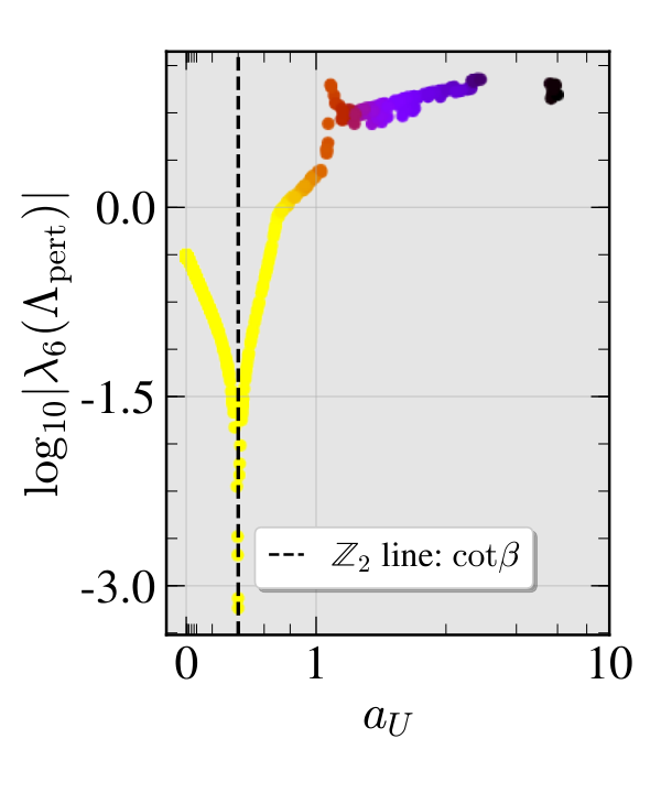
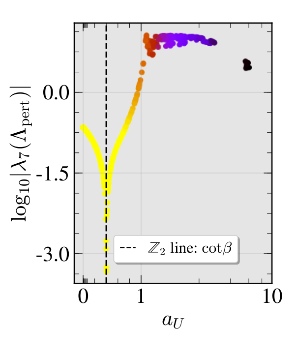

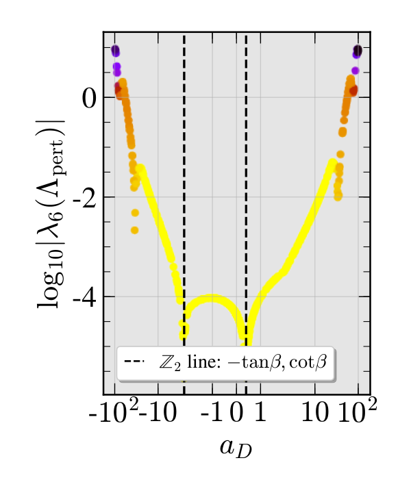
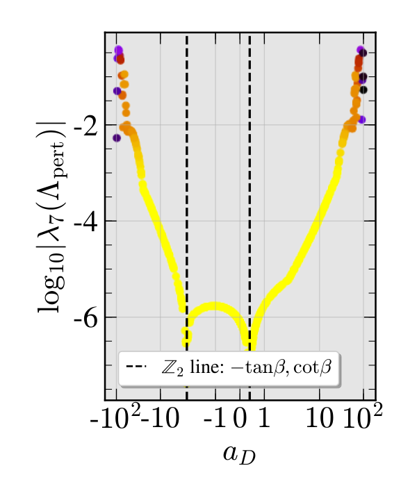

In scenario IV.a we separately vary each one-by-one, while keeping the other fixed, with the scalar potential in eq. (3.4), see figure 11. The symmetric values, and or , are clearly visible and are displayed as vertical lines. As expected, the up-sector is much more sensitive because of the large top Yukawa coupling. sizable non-diagonal FCNCs can be generated by deviating from the symmetric values in both the up and down sector. We especially note that, perturbativity in the scalar potential easily breaks down for large deviations of in the up sector.
When varying , the maximum generated FCNC occurs for a value , where . In this region, can become very large, , without perturbativity breaking down. The phenomenon that the maximum occurs when is general and is more clearly visible in figure 14 below.
Example from scenario IV.a
To illustrate the RG evolution, an example parameter point from scenario IV.a with the alignment coefficients , is shown in figure 12. Stability breaks down for this parameter space point already at 1 TeV, but as before we ignore that.
Scenario IV.b


In scenario IV.b, we perform a random parameter scan of a 2HDM with a softly broken potential, just as in scenario II, but fix . Furthermore, here we also vary the alignment parameters in the quark sector, . This way we get a quantitative estimate of the induced breaking parameters and . As discussed earlier, we only keep parameter points that satisfies all theoretical constraints during the entire RG running up to GeV.
The induced are shown for a scan of surviving parameter points in figure 13. It is clear that the generated breaking parameters are more sensitive to variations in , because of the large top Yukawa coupling. Note the vertical area around which gives the smallest .
As previously mentioned, it is the which is the largest generated non-diagonal element in more than of all cases; therefore we use it as a measure of the induced FCNCs in figure 14. The dark regions, where the smallest FCNCs are generated, arise since the relations and correspond to an aligned Yukawa sector that is 1-loop stable under RG evolution Ferreira:2010xe. Even though these relations imply that there is a symmetric Yukawa sector in one particular basis, at 2-loop order the scalar and Yukawa sectors mix and induce FCNCs if the do not take on the correct symmetric values set by the scalar potential. We also note the region , where the maximum FCNCs are generated; similar to what was seen when varying separately in figure 11.
 |
5 Conclusions
We have derived the complete set of 2-loop RGEs for a general, potentially complex, 2HDM and implemented them in the C++ code 2HDME Oredsson:2018vio. Using this software, we performed a RG analysis of the -conserving 2HDM and investigated the parameter space with different levels of symmetry (exact, soft or hard breaking). The case of a softly broken symmetry is the most unconstrained type of 2HDM, since it allows for large scalar masses, larger values of and we found regions in the parameter space with models that are valid all the way up to the Planck scale.
Breaking the symmetry hard at the EW scale induces dimensionless breaking parameters during the RG running which can be potentially dangerous and severely limit the validity of the model. We have looked at two scenarios, where we have either broken the symmetry hard in the scalar potential, by having non-zero , or in the Yukawa sector, by making a flavor Yukawa ansatz at the EW scale.
We have found that for at the EW scale, it is possible to find models that are valid all the way up to the Planck scale at GeV; while models break down already at GeV if . The generated FCNCs, that spread from the scalar sector first at 2-loop order, are however heavily suppressed.
A flavor ansatz can be a viable solution to the FCNC problem, even though it is not protected during RG evolution. Deviations of from the symmetric limit, , or , should however not be too large. The up sector is especially sensitive when it comes to induced ; which contribute to a rapid growth of the quartic couplings. In the down sector, the induced FCNCs pose the primary limitation. Finally we observe that there is a region in the flavor alignment parameter space, , which gives the maximum FCNCs. The origin of this effect is unclear and requires further study.
Acknowledgements.
The authors would like to thank Hugo Serodio and Johan Bijnens for useful discussions. This work is supported in part by the Swedish Research Council grants contract numbers 621-2013-4287 and 2016-05996 and by the European Research Council (ERC) under the European Union’s Horizon 2020 research and innovation programme (grant agreement No 668679).Appendix A Quartic couplings in scenario II
The quartic couplings in the random parameter scan of scenario II with a softly broken symmetry, described in section 4.2, as functions of breakdown energy in RG evolution are shown in the generic basis in figure 15 and in the Higgs basis in figure 16. The color coding is the maximum breakdown-energy from perturbativity, unitarity or stability in each bin.
Generic basis


 .
.
Higgs basis, Scenario II


Appendix B Tree-level unitarity conditions
The tree-level unitarity conditions for a general 2HDM have been worked out in ref. Ginzburg:2005dt. There, they work out the following scattering matrices:
| (57) | ||||
In the end, the unitarity constraint puts upper limits on the absolute value of the eigenvalues, , of these matrices,
| (66) |
Appendix C Tree-level stability
Here, we give the conditions for the tree-level scalar potential to be bounded from below, as worked out in ref. Ivanov:2006yq; Ivanov:2007de.
When working out these conditions, ref. Ivanov:2006yq; Ivanov:2007de constructed a Minkowskian formalism of the 2HDM that uses gauge-invariant field bilinears,
| (67) | ||||
| (68) | ||||
| (69) | ||||
| (70) |
These can be used to create a four-vector ; where one can raise and lower the indices as usual with the flat Minkowski metric . In this formalism, the scalar potential is conveniently written as
| (71) |
where
| (72) |
and
The scalar potential is bounded from below if and only if all of the below requirements are fulfilled:
- •
All the eigenvalues of are real.
- •
There exists a largest eigenvalue that is positive, and .
- •
There exist four linearly independent eigenvectors; one for each eigenvalue .
- •
The eigenvector corresponding to the largest eigenvalue is timelike, while the others are spacelike,
(77) (78)
References
- (1) ATLAS Collaboration, G. Aad et. al., Observation of a new particle in the search for the Standard Model Higgs boson with the ATLAS detector at the LHC, Phys. Lett. B716 (2012) 1–29, [arXiv:1207.7214].
- (2) CMS Collaboration, S. Chatrchyan et. al., Observation of a new boson at a mass of 125 GeV with the CMS experiment at the LHC, Phys. Lett. B716 (2012) 30–61, [arXiv:1207.7235].
- (3) ATLAS, CMS Collaboration, G. Aad et. al., Measurements of the Higgs boson production and decay rates and constraints on its couplings from a combined ATLAS and CMS analysis of the LHC pp collision data at and 8 TeV, JHEP 08 (2016) 045, [arXiv:1606.02266].
- (4) G. Branco, P. Ferreira, L. Lavoura, M. Rebelo, M. Sher, et. al., Theory and phenomenology of two-Higgs-doublet models, Phys.Rept. 516 (2012) 1–102, [arXiv:1106.0034].
- (5) S. L. Glashow and S. Weinberg, Natural Conservation Laws for Neutral Currents, Phys. Rev. D15 (1977) 1958.
- (6) E. A. Paschos, Diagonal Neutral Currents, Phys. Rev. D15 (1977) 1966.
- (7) P. Bechtle, O. Brein, S. Heinemeyer, G. Weiglein, and K. E. Williams, HiggsBounds: Confronting Arbitrary Higgs Sectors with Exclusion Bounds from LEP and the Tevatron, Comput. Phys. Commun. 181 (2010) 138–167, [arXiv:0811.4169].
- (8) P. Bechtle, O. Brein, S. Heinemeyer, G. Weiglein, and K. E. Williams, HiggsBounds 2.0.0: Confronting Neutral and Charged Higgs Sector Predictions with Exclusion Bounds from LEP and the Tevatron, Comput. Phys. Commun. 182 (2011) 2605–2631, [arXiv:1102.1898].
- (9) P. Bechtle, O. Brein, S. Heinemeyer, O. Stål, T. Stefaniak, G. Weiglein, and K. E. Williams, : Improved Tests of Extended Higgs Sectors against Exclusion Bounds from LEP, the Tevatron and the LHC, Eur. Phys. J. C74 (2014), no. 3 2693, [arXiv:1311.0055].
- (10) P. Bechtle, S. Heinemeyer, O. Stål, T. Stefaniak, and G. Weiglein, : Confronting arbitrary Higgs sectors with measurements at the Tevatron and the LHC, Eur. Phys. J. C74 (2014), no. 2 2711, [arXiv:1305.1933].
- (11) A. Pich and P. Tuzon, Yukawa Alignment in the Two-Higgs-Doublet Model, Phys. Rev. D80 (2009) 091702, [arXiv:0908.1554].
- (12) A. Peñuelas and A. Pich, Flavour alignment in multi-Higgs-doublet models, JHEP 12 (2017) 084, [arXiv:1710.02040].
- (13) M. Jung, A. Pich, and P. Tuzon, Charged-Higgs phenomenology in the Aligned two-Higgs-doublet model, JHEP 11 (2010) 003, [arXiv:1006.0470].
- (14) P. M. Ferreira, L. Lavoura, and J. P. Silva, Renormalization-group constraints on Yukawa alignment in multi-Higgs-doublet models, Phys. Lett. B688 (2010) 341–344, [arXiv:1001.2561].
- (15) F. J. Botella, G. C. Branco, A. M. Coutinho, M. N. Rebelo, and J. I. Silva-Marcos, Natural Quasi-Alignment with two Higgs Doublets and RGE Stability, Eur. Phys. J. C75 (2015) 286, [arXiv:1501.07435].
- (16) J. Bijnens, J. Lu, and J. Rathsman, Constraining General Two Higgs Doublet Models by the Evolution of Yukawa Couplings, JHEP 1205 (2012) 118, [arXiv:1111.5760].
- (17) P. S. Bhupal Dev and A. Pilaftsis, Maximally Symmetric Two Higgs Doublet Model with Natural Standard Model Alignment, JHEP 12 (2014) 024, [arXiv:1408.3405]. [Erratum: JHEP11,147(2015)].
- (18) P. Ferreira, H. E. Haber, and E. Santos, Preserving the validity of the Two-Higgs Doublet Model up to the Planck scale, Phys. Rev. D92 (2015) 033003, [arXiv:1505.04001]. [Erratum: Phys. Rev.D94,no.5,059903(2016)].
- (19) S. Gori, H. E. Haber, and E. Santos, High scale flavor alignment in two-Higgs doublet models and its phenomenology, JHEP 06 (2017) 110, [arXiv:1703.05873].
- (20) P. Basler, P. M. Ferreira, M. Mühlleitner, and R. Santos, High scale impact in alignment and decoupling in two-Higgs doublet models, Phys. Rev. D97 (2018), no. 9 095024, [arXiv:1710.10410].
- (21) F. J. Botella, F. Cornet-Gomez, and M. Nebot, Flavour Conservation in Two Higgs Doublet Models, arXiv:1803.08521.
- (22) D. Chowdhury and O. Eberhardt, Global fits of the two-loop renormalized Two-Higgs-Doublet model with soft Z2 breaking, JHEP 11 (2015) 052, [arXiv:1503.08216].
- (23) J. Braathen, M. D. Goodsell, M. E. Krauss, T. Opferkuch, and F. Staub, -loop running should be combined with -loop matching, Phys. Rev. D97 (2018), no. 1 015011, [arXiv:1711.08460].
- (24) M. E. Krauss, T. Opferkuch, and F. Staub, The Ultraviolet Landscape of Two-Higgs Doublet Models, arXiv:1807.07581.
- (25) A. V. Bednyakov, On Three-loop RGE for the Higgs Sector of 2HDM, arXiv:1809.04527.
- (26) J. Oredsson, 2 Higgs Doublet Model Evolver - Manual, arXiv:1811.08215.
- (27) S. Davidson and H. E. Haber, Basis-independent methods for the two-Higgs-doublet model, Phys. Rev. D72 (2005) 035004, [hep-ph/0504050]. [Erratum: Phys. Rev.D72,099902(2005)].
- (28) H. E. Haber and D. O’Neil, Basis-independent methods for the two-Higgs-doublet model. II. The Significance of tan, Phys. Rev. D74 (2006) 015018, [hep-ph/0602242]. [Erratum: Phys. Rev.D74,no.5,059905(2006)].
- (29) H. E. Haber and D. O’Neil, Basis-independent methods for the two-Higgs-doublet model III: The CP-conserving limit, custodial symmetry, and the oblique parameters S, T, U, Phys. Rev. D83 (2011) 055017, [arXiv:1011.6188].
- (30) G. C. Branco, L. Lavoura, and J. P. Silva, CP Violation, Int. Ser. Monogr. Phys. 103 (1999) 1–536.
- (31) T. P. Cheng and M. Sher, Mass-matrix ansatz and flavor nonconservation in models with multiple higgs doublets, Phys. Rev. D 35 (Jun, 1987) 3484–3491.
- (32) J. F. Gunion and H. E. Haber, Conditions for CP-violation in the general two-Higgs-doublet model, Phys. Rev. D72 (2005) 095002, [hep-ph/0506227].
- (33) L. Lavoura and J. P. Silva, Fundamental CP violating quantities in a SU(2) x U(1) model with many Higgs doublets, Phys. Rev. D50 (1994) 4619–4624, [hep-ph/9404276].
- (34) F. J. Botella and J. P. Silva, Jarlskog - like invariants for theories with scalars and fermions, Phys. Rev. D51 (1995) 3870–3875, [hep-ph/9411288].
- (35) H. E. Haber and O. Stål, New LHC benchmarks for the -conserving two-Higgs-doublet model, Eur. Phys. J. C75 (2015), no. 10 491, [arXiv:1507.04281]. [Erratum: Eur. Phys. J.C76,no.6,312(2016)].
- (36) I. F. Ginzburg and I. P. Ivanov, Tree-level unitarity constraints in the most general 2HDM, Phys. Rev. D72 (2005) 115010, [hep-ph/0508020].
- (37) I. P. Ivanov, Minkowski space structure of the Higgs potential in 2HDM, Phys. Rev. D75 (2007) 035001, [hep-ph/0609018]. [Erratum: Phys. Rev.D76,039902(2007)].
- (38) I. P. Ivanov, Minkowski space structure of the Higgs potential in 2HDM. II. Minima, symmetries, and topology, Phys. Rev. D77 (2008) 015017, [arXiv:0710.3490].
- (39) D. Eriksson, J. Rathsman, and O. Stål, 2HDMC: Two-Higgs-Doublet Model Calculator Physics and Manual, Comput. Phys. Commun. 181 (2010) 189–205, [arXiv:0902.0851].
- (40) F. Staub, SARAH, arXiv:0806.0538.
- (41) F. Staub, SARAH 4 : A tool for (not only SUSY) model builders, Comput. Phys. Commun. 185 (2014) 1773–1790, [arXiv:1309.7223].
- (42) F. Lyonnet, I. Schienbein, F. Staub, and A. Wingerter, PyR@TE: Renormalization Group Equations for General Gauge Theories, Comput. Phys. Commun. 185 (2014) 1130–1152, [arXiv:1309.7030].
- (43) I. Schienbein, F. Staub, T. Steudtner, and K. Svirina, Revisiting RGEs for general gauge theories, arXiv:1809.06797.
- (44) M. E. Machacek and M. T. Vaughn, Two Loop Renormalization Group Equations in a General Quantum Field Theory. 1. Wave Function Renormalization, Nucl. Phys. B222 (1983) 83–103.
- (45) M. E. Machacek and M. T. Vaughn, Two Loop Renormalization Group Equations in a General Quantum Field Theory. 2. Yukawa Couplings, Nucl. Phys. B236 (1984) 221–232.
- (46) M. E. Machacek and M. T. Vaughn, Two Loop Renormalization Group Equations in a General Quantum Field Theory. 3. Scalar Quartic Couplings, Nucl. Phys. B249 (1985) 70–92.
- (47) M.-x. Luo, H.-w. Wang, and Y. Xiao, Two loop renormalization group equations in general gauge field theories, Phys. Rev. D67 (2003) 065019, [hep-ph/0211440].
- (48) I. F. Ginzburg, Necessity of mixed kinetic term in the description of general system with identical scalar fields, Phys. Lett. B682 (2009) 61–66, [arXiv:0810.1546].
- (49) J. Bijnens, J. Oredsson, and J. Rathsman, Scalar Kinetic Mixing and the Renormalization Group, arXiv:1810.04483.
- (50) M. G. et.al., GNU Scientific Library Reference Manual (3rd Ed.), ISBN 0954612078 [http://www.gnu.org/software/gsl/].
- (51) G. Guennebaud, B. Jacob, et. al., “Eigen v3.” http://eigen.tuxfamily.org, 2010.
- (52) ATLAS, CDF, CMS, D0 Collaboration, First combination of Tevatron and LHC measurements of the top-quark mass, arXiv:1403.4427.
- (53) Z.-z. Xing, H. Zhang, and S. Zhou, Updated Values of Running Quark and Lepton Masses, Phys. Rev. D77 (2008) 113016, [arXiv:0712.1419].
- (54) D. Buttazzo, G. Degrassi, P. P. Giardino, G. F. Giudice, F. Sala, A. Salvio, and A. Strumia, Investigating the near-criticality of the Higgs boson, JHEP 12 (2013) 089, [arXiv:1307.3536].
- (55) Particle Data Group Collaboration, M. T. et al., Review of Particle Physics, Phys. Rev. D98 (2018) 030001.
- (56) W. Porod, SPheno, a program for calculating supersymmetric spectra, SUSY particle decays and SUSY particle production at e+ e- colliders, Comput. Phys. Commun. 153 (2003) 275–315, [hep-ph/0301101].
- (57) W. Porod and F. Staub, SPheno 3.1: Extensions including flavour, CP-phases and models beyond the MSSM, Comput. Phys. Commun. 183 (2012) 2458–2469, [arXiv:1104.1573].
- (58) D. Das and I. Saha, Search for a stable alignment limit in two-Higgs-doublet models, Phys. Rev. D91 (2015), no. 9 095024, [arXiv:1503.02135].