Prefix-Free Code Distribution Matching for Probabilistic Constellation Shaping

The $m$-out-of-$n$ coding [14] and the constant composition DM (CCDM) [15] are fixed-to-fixed length (F2F) DMs that realize a target code symbol distribution on a block-by-block basis using arithmetic coding. The CCDM was shown to be asymptotically optimal in the sense that the normalized Kullback-Leibler (KL) divergence between the desired and realized symbol distributions vanishes as the block length goes to infinity [15]. The computational complexity of CCDM increases linearly with the block length, making it possible to use a very large block length to closely approach the asymptotic performance. However, CCDM requires high-precision multiplications and divisions. In [16], the multiset partitioning DM (MPDM) was proposed to enhance the degrading performance of CCDM in small blocks, by letting CCDM create different symbol distributions across multiple blocks that are averaged to the target distribution. For a small block length, typically below 100 symbols, there have been algorithmic approaches to implement an F2F DM, such as the shell mapping [17, 18, 19] and the enumerative sphere shaping [20]. The algorithmic approaches substantially reduced the complexity of indexing a point in a sphere, by divide and conquer [17, 18, 19] or dynamic programming[20], which is otherwise exponential in the dimension. Nevertheless, their complexity is polynomial in the dimension, e.g., quadratic for the Algorithm 2 of [18], hence a large block length cannot be used. More recently, an F2F DM was realized in [21] by using a distribution uniformizer that makes all the symbols in a code alphabet appear the same number of times in each block, followed by run-length coding that transforms the uniform distribution into a non-uniform target distribution.

It was recently shown that F2F DMs like $m$-out-of-$n$ [14] and CCDM [15] cannot fundamentally eliminate the un-normalized KL divergence between the desired and realized symbol distributions [22]. On the other hand, variable-length may achieve zero un-normalized KL divergence [1]. Importantly, variable-length PCDM has a linear complexity in the dimension, as in CCDM and the run-length coding [21], hence can be realized in large dimensions to achieve zero un-normalized KL divergences. Furthermore, unlike the $m$-out-of-$n$ or CCDM, PCDM does not require high-precision arithmetic. To this end, we limit the scope to variable-length prefix-free codes and study the construction of prefix-free codes for rate-adaptable PCDM throughout the paper.

Let $\bm{b}$ and $\bm{x}$, respectively, denote a concatenation of an indefinite number of information symbols drawn from the binary alphabet $\mathcal{B}$ and a concatenation of an indefinite number of code symbols drawn from the ASK alphabet $\mathcal{X}$. Then, a code $\mathcal{C}:\bm{\mathcal{B}}\mapsto\bm{\mathcal{X}}$ defines a bijective function that maps every information word $\bm{b}$ in the dictionary $\bm{\mathcal{B}}$ to a codeword $\bm{x}$ in the codebook $\bm{\mathcal{X}}$. If the codeword $\bm{x}\in\bm{\mathcal{X}}$ is an ordered concatenation of two words $\bm{x}_{\mathrm{pre}}$ and $\bm{x}^{\prime}$, then $\bm{x}_{\mathrm{pre}}$ is called a prefix of the word $\bm{x}$. A code is a prefix-free code if any codeword $\bm{x}\in\bm{\mathcal{X}}$ is not a prefix of another codeword. A prefix-free code is an instantaneously decodable code, whose decoding can be performed as immediately as a codeword is found on successive receipt of the code symbols.

In a special case where all code symbols in $\mathcal{X}$ have equal transmit energies, and if the information word distribution is known a priori, Huffman codes represent optimal prefix-free codes in the sense that no other codes can produce a shorter expected codeword length, hence a smaller average code symbol energy. In a more general case where the energies of symbols in $\mathcal{X}$ are not necessarily equal, the prefix-free code construction problem has been addressed in the context of PCS [23], using Lempel-Even-Cohn (LEC) coding [24] and Varn coding [3]. LEC coding solves the problem when all codewords have an equal length. LEC coding is isomorphic to Huffman coding if we convert the energy of a codeword into the probability of the corresponding information word. A Huffman codebook therefore becomes the LEC dictionary for parsing information bits, mapped to an LEC codebook that consists of equal-length codewords, completing a variable-to-fixed length (V2F) code. However, while we want to minimize the energy per code symbol for arbitrary resolution rates, LEC coding minimizes the energy per information symbol, and its resolution rate is determined by the Huffman codebook that is given a priori. Varn coding provides another solution when information words have an equal length, hence constructing fixed-to-variable length (F2V) codes. However, Varn coding requires a non-uniform probability mass function (PMF) for the equal-length information words, which must be given a priori to realize a particular resolution rate. Another approach to constructing F2V codes is by minimizing the KL divergence between the desired and realized PMFs for a binary code alphabet [25], which also assumes a priori knowledge of the optimal PMF for the target resolution rate. In general cases where both information words and codewords can have unequal lengths, there are known algorithms to construct optimal prefix-free codes [4, 26, 27, 28, 29] using, e.g., dynamic programming [28, 29]. However, they require unequal probabilities of the information symbols that must be given a priori, and the resulting codes are optimal only in the sense that they minimize the average codeword energy, without taking into account the resolution rate. To the best of our knowledge, none of the existing approaches addressed the problem of constructing prefix-free codes to minimize the average code symbol energy for arbitrary target resolution rates.

To solve problem (III), we begin with a balanced $M$-ary right tree, i.e., a right tree in which every branch has $M$ children and every leaf is at the same depth (see the right tree of Fig. 1 (a)), which represents a codebook $\bm{\mathcal{X}}$ with a fixed codeword length $l(\bm{x})=v$ for all $\bm{x}\in\bm{\mathcal{X}}$. Then, the codebook can immediately be obtained from the fixed codeword length $v$ by lexicographical ordering as $\bm{\mathcal{X}}_{v}=\mathcal{X}_{M\textrm{-ASK}}^{v}$, and $|\mathcal{C}|=M^{v}$. In this case, (1) and (2) degenerate, respectively, to

and

where the last equation holds since $\mathbb{P}_{\bm{X}}$ is dyadic. Therefore, for V2F codes, minimizing the average code symbol energy is equivalent to minimizing the average codeword energy. Also, maximizing $\mathsf{R}_{\mathcal{C}}$ subject to $\mathsf{E}_{\mathcal{C}}\leq\mathsf{E}^{*}$ is equivalent to maximizing $\mathbb{H}(\bm{X})$ subject to $\mathbb{E}(||\bm{X}||^{2})\leq v\mathsf{E}^{*}$.

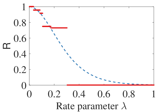
If we waive the dyadic constraint on $\mathbb{P}_{\bm{X}}$, the entropy $\mathbb{H}(\bm{X})$ is maximized by $\bm{X}_{\text{MB}}$ that follows an MB distribution $\mathbb{P}_{\bm{X}_{\text{MB}}}(\bm{x}):=\exp(-\lambda||\bm{x}||^{2})/\sum_{\bm{x}\in\bm{\mathcal{\bm{X}}}}\exp(-\lambda||\bm{x}||^{2})$. Note that $\bm{X}_{\text{MB}}$ is a random vector, whereas $X_{\text{MB}}$ in (III) is a random scalar. Since $||\bm{x}||^{2}=\sum_{x\in\bm{x}}|x|^{2}$, we have that $\mathbb{P}_{\bm{X}_{\text{MB}}}(\bm{x})=\prod_{x\in{\bm{x}}}\mathbb{P}_{X_{\text{MB}}}(x)$. We also have that $\mathbb{H}(\bm{X}_{\text{MB}})=v\mathbb{H}(X_{\text{MB}})$. Therefore, if a dictionary $\bm{\mathcal{B}}$ can make the codewords $\bm{X}$ follow the distribution $\mathbb{P}_{\bm{X}_{\text{MB}}}$, the code achieves both $\mathsf{E}_{\mathcal{C}}=\mathbb{E}(|X_{\text{MB}}|^{2})$ and $\mathsf{R}_{\mathcal{C}}=\mathbb{H}(X_{\text{MB}})$. Indeed, LEC coding [24] is optimal in the sense that it yields a special instance of the MB distribution, for which the rate parameter is given by $\lambda=\log(\beta)$ with $\beta$ being a root of the characteristic condition $\sum_{\bm{x}\in\bm{\mathcal{X}}}\beta^{-||\bm{x}||^{2}}=1$. The dashed curves in Fig. 2 (a) and (b) show the average symbol energy and the entropy rate of $X_{\text{MB}}$ as a strictly monotonically decreasing function of $\lambda$ (this is true in general, see [13, Section 5.C]), obtained from the codewords of Tab. I (a). Due to the monotonicity, the rate parameter $\lambda$ of the MB PMF $\mathbb{P}_{\bm{X}_{\text{MB}}}$ that leads to the minimum average symbol energy $\mathbb{E}(|X_{\text{MB}}|^{2})$ subject to the rate constraint $\mathbb{H}(X_{\text{MB}})=\mathsf{R}^{*}$ can simply be obtained by the bisection method. Once we obtain $\mathbb{P}_{\bm{X}_{\text{MB}}}$, its optimal dyadic approximate $\mathbb{P}_{\widetilde{\bm{X}}_{\text{MB}}}$ can be obtained by Geometric Huffman coding (GHC) [30], i.e., $\mathbb{P}_{\widetilde{\bm{X}}_{\text{MB}}}=\text{GHC}(\mathbb{P}_{\bm{X}_{\text{MB}}})$, optimal in the sense that it minimizes the KL divergence $\mathbb{D}(\mathbb{P}_{\widetilde{\bm{X}}_{\text{MB}}}\|\mathbb{P}_{\bm{X}_{\text{MB}}}):=\sum_{\bm{x}\in\bm{\mathcal{X}}}\mathbb{P}_{\widetilde{\bm{X}}_{\text{MB}}}(\bm{x})\log_{2}\frac{\mathbb{P}_{\widetilde{\bm{X}}_{\text{MB}}}(\bm{x})}{\mathbb{P}_{\bm{X}_{\text{MB}}}(\bm{x})}$. Notice that, since $\mathcal{X}$ and $v$ completely define the right tree $\bm{\mathcal{X}}_{v}$, the PMF $\mathbb{P}_{\bm{X}_{\text{MB}}}$ can immediately be obtained for an arbitrary target resolution rate $\mathsf{R}^{*}$, using a series of operations $(\mathcal{X},v,\mathsf{R}^{*})\mapsto\mathbb{P}_{\bm{X}_{\text{MB}}}\mapsto\mathbb{P}_{\widetilde{\bm{X}}_{\text{MB}}}\mapsto(\bm{\mathcal{B}},\bm{\mathcal{X}}_{v})$. The solid lines in Fig. 2 show the average symbol energy and resolution rate that can be obtained using this method for $\mathcal{X}_{2\text{-ASK}}$ with $v=3$. In this example, there are only five non-zero distinct resolution rates generated by the dyadic PMF $\mathbb{P}_{\widetilde{\bm{X}}_{\text{MB}}}$.

However, as $v$ increases, the created codes have much finer granularity of the resolution rate, as shown in Fig. 3 for up to the 16-ASK alphabet (producing up to the 1024-QAM in the PAS architecture). Here, we find all V2F codes of the cardinality $|\mathcal{C}|\leq 4096$ for the target resolution rates $\mathsf{R}^{*}\in\{\Delta,2\Delta,\ldots,\log_{2}M\}$ with rate granularity $\Delta=0.001$. The codes have less finer granularity of the resolution rate in the lower resolution rate regime, which can be supplemented by allowing variable codeword lengths, as will be discussed in Section III-C. Figure 3 shows that the constructed V2F codes achieve energy gaps smaller than 0.1 dB across a wide range of resolution rates with a cardinality $|\mathcal{C}|\leq 4096$, or even $|\mathcal{C}|\leq 64$ for $M\leq 4$.

For F2V codes, we consider a balanced binary left tree representing a dictionary $\bm{\mathcal{B}}$ with a fixed information word length $l(\bm{b})=u$ for all $\bm{b}\in\bm{\mathcal{B}}$ such that $|\mathcal{C}|=2^{u}$. Then, the dictionary $\bm{\mathcal{B}}_{u}$ can be immediately obtained by lexicographical ordering of $\mathcal{B}^{u}$, and all the information words $\bm{b}\in\bm{\mathcal{B}}_{u}$ are parsed to the codewords $\bm{x}\in\bm{\mathcal{X}}$ with the equal probability $\mathbb{P}_{\bm{B}}(\bm{b})=2^{-u}$. Let us define the sum depth and sum energy of a right tree as $l(\bm{\mathcal{X}}):=\sum_{\bm{x}\in\bm{\mathcal{X}}}l(\bm{x})$ and $||\bm{\mathcal{X}}||^{2}:=\sum_{\bm{x}\in\bm{\mathcal{X}}}||\bm{x}||^{2}$, respectively. Then, the average symbol energy and the resolution rate of the code are calculated, respectively, as

and

We do not know of any existing method that can solve (III) with (6) and (7) for an arbitrary desired $\mathsf{R}^{*}$. In this paper, therefore, instead of directly solving the problem for a particular $\mathsf{R}^{*}$, we try to identify a set of trees that produces all possible sum depths $l(\bm{\mathcal{X}})$ under a tree size constraint $|\bm{\mathcal{X}}|=u$, hence realizing all possible $\mathsf{R}_{\mathcal{C}}$ according to (7). The constructed trees are optimal in the sense that they have the minimum sum energy $||\bm{\mathcal{X}}||^{2}$ among all $2^{+}$-trees with the same sum depth $l(\bm{\mathcal{X}})$, where $L^{+}$-tree is a tree in which every node except leaves has a degree not smaller than $L$. This further implies that the tree achieves the minimum average symbol energy $\mathsf{E}_{\mathcal{C}}$ for the given $l(\bm{\mathcal{X}})$ and $\mathsf{R}_{\mathcal{C}}$ due to (6) and (7). Indeed, any $1^{+}$-tree is allowed for a right tree; however, we restrict the type of trees to $2^{+}$-trees to avoid infinite tree expansion (see Fig. 4 (a) for example). In Fig. 4, and throughout the paper, $\mathcal{T}(N)$ denotes a right tree that has $N$ leaves, i.e., $|\bm{\mathcal{X}}|=N$, $\mathcal{T}(N,\nu)$ is a tree $\mathcal{T}(N)$ whose sum depth $l(\bm{\mathcal{X}})=v$, and $\mathcal{T}(N,\nu,\omega)$ is a tree $\mathcal{T}(N,\nu)$ whose sum energy $||\bm{\mathcal{X}}||^{2}=\omega$. Also, let $\bm{\Psi}(N)$ and $\bm{\Psi}(N,\nu)$ be the sets of all trees $\mathcal{T}(N)$ and $\mathcal{T}(N,\nu)$, respectively. Then, by (6) and (7), all trees in $\bm{\Psi}(N,\nu)$ lead to the same $\mathsf{R}_{\mathcal{C}}$ but not necessarily the same $\mathsf{E}_{\mathcal{C}}$. Since a distinct sum depth $\nu$ generates a distinct $\mathsf{R}_{\mathcal{C}}=2^{u}u/\nu$ for the fixed $u$, we have as many optimal trees as the number of distinct sum depths of trees in $\bm{\Psi}(N)$, where an optimal tree with sum depth $\nu$ is defined as $\mathcal{T}^{*}(N,\nu)=\argmin_{\mathcal{T}(N,\nu)\in\bm{\Psi}(N,\nu)}||\bm{\mathcal{X}}||^{2}$. A brute-force search of $\mathcal{T}^{*}(N,\nu)$ in $\bm{\Psi}(N)$ requires exponential time in $N$. There are known problems that are isomorphic to the problem of counting the number of all trees in $\bm{\Psi}(N)$, including the parenthesizations counting problem [31, Ch. 15.2]. For example, the trees in $\bm{\Psi}(4)$ of Fig. 4 (b) have isomorphic representations of $((13)(13))$, $(((13)3)3)$, $((1(13))3)$, $(1((13)3))$, and $(1(1(13)))$ in order, in which the edges connecting two siblings are parenthesized together in a recursive manner from the largest depth of the tree. The number of parenthesizations for $\bm{\Psi}(N)$ is $C_{N-1}$, with $C_{N}$ being the Catalan number defined as $C_{N}:=\frac{(2N)!}{N!(N+1)!}$ [32, 33], which grows as $\Omega(\frac{4^{N}}{N^{3/2}})$ [31, p. 333].

In order to reduce the search space, we take a dynamic programming approach, as in [28, 29], to find a prefix-free code for a known codeword PMF.

We begin from a trivial size-1 tree that has only a root, then construct larger trees by appending smaller trees to the root, as shown in Fig. 5. A tree $\mathcal{T}(N,\nu,\omega)$ formed by appending sub-trees $\mathcal{T}(N_{j},\nu_{j},\omega_{j})$, $j=1,\ldots,J$ satisfies the following relations:

where the last two equations hold since the $j$-th edge from the root should be taken into account $N_{j}$ times to calculate sum depth and sum energy of the tree. For example, due to (8), a tree of $N=4$ with the $4$-ASK alphabet (hence $2\leq J\leq 4$) can be constructed from $J$-tuples: $(N_{1},N_{2})=(1,3),(2,2),(3,1)$ for $J=2$, $(N_{1},N_{2},N_{3})=(1,1,2),(1,2,1),(2,1,1)$ for $J=3$, and $(N_{1},N_{2},N_{3},N_{4})=(1,1,1,1)$ for $J=4$. Here, we do not need to use all sub-trees of size $<N$ to construct a set of size-$N$ trees, since we have an optimal sub-substructure property:

It can be easily seen that the height of $\mathcal{T}(N)$ is minimized when its leaves have maximally uniform depths. The depths can differ from each other at most by one, and the minimum height is given by $\lceil\log_{M}N\rceil$ for the $M$-ASK alphabet. The sum depth of a size-$N$ minimum-height tree is calculated as $\nu_{\text{min}}:=(N-M^{\lfloor\log_{M}N\rfloor})(\lfloor\log_{M}N\rfloor+1)+M^{\lfloor\log_{M}N\rfloor}\lfloor\log_{M}N\rfloor$, which is equal to the smallest sum depth of all trees in $\bm{\Psi}(N)$. If $N$ is a positive integer power of $M$, the minimum sum depth can be simplified as $\nu_{\text{min}}=N\log_{M}N$. On the other hand, if there are only two nodes at every depth of a tree (see, e.g., the last tree of Fig. 4 (b)), the tree has height $N-1$ that is the largest of all trees in $\bm{\Psi}(N)$. The sum depth in this case is calculated as $\nu_{\text{max}}=\sum_{v=1}^{N-1}v+(N-1)=\frac{(N+2)(N-1)}{2}$. After some manipulation, it can be seen that the sum depth of a maximum-height tree is also the maximum sum depth of all trees in $\bm{\Psi}(N)$. Therefore, if we store only one optimal tree to $\bm{\Psi}^{*}(N)$ for each $\nu$, the size of $\bm{\Psi}^{*}(N)$ is upper-bounded by $\nu_{\text{max}}-\nu_{\text{min}}+1=\frac{N^{2}}{2}+O(N\log_{M}N)$; i.e., $|\bm{\Psi}^{*}(N)|$ grows as $O(N^{2})$. Since there are at most $N$ choices of the optimal sub-tree sets (ranging from an empty set to $\bm{\Psi}^{*}(N-1)$) for each of the $M$ edges of the root for enumerating all trees of size $N$ (using the optimal sub-tree property), the number of all choices to build $\bm{\Psi}(N)$ is of the complexity $\Omega(N^{M})$. As aforementioned, each of the sub-tree sets is of size at most $\Omega(N^{2})$, hence we have the search space of size $\Omega(N^{M+2})$ to identify $\bm{\Psi}^{*}(N)$. The search time is polynomial in $N$, and exponential in $M$, indicating the intractability of constructing F2V codes for a large alphabet.

To further reduce the search space, we can exploit the fact that a larger sub-tree is appended as far left as possible from the root of an optimal tree; i.e.,

We construct one optimal F2V code for each of the resolution rates that can be created with $N\leq 64$ for $\mathcal{X}_{\text{2-ASK}}$ and $\mathcal{X}_{\text{4-ASK}}$. As shown in Fig. 6, F2V codes offer finer granularity of the resolution rates than V2F codes with the same cardinality, albeit with a slightly larger energy gap. Therefore, a natural consequence is to construct V2V codes to exploit the complementary merits of V2F and F2V codes, as will be illustrated henceforth.

We readily have a set $\bm{\Psi}_{\text{R}}^{*}(N)$ of optimal right trees, representing optimal F2V codes. From this, without imposing any length constraints on information words and codewords, we can enumerate near-optimal V2V codes of the cardinality $|\mathcal{C}|=N$ in the following manner:

1. 1.

   For each of the desired resolution rates $\mathsf{R}^{*}=j\Delta_{\mathsf{R}}$, where $j=1,\ldots,J$ for some integer $J$ and the rate granularity $\Delta_{\mathsf{R}}=\frac{\log_{2}M}{J}$, and for each of the optimal right trees in $\bm{\Psi}_{\text{R}}^{*}$, identify the MB PMF $\mathbb{P}_{\bm{X}_{\text{MB}}}$ that fulfills $\mathbb{H}(X_{\text{MB}})=\mathsf{R}^{*}$.

2. 2.

   For every $\mathbb{P}_{\bm{X}_{\text{MB}}}$ obtained in Step 1, construct a set of optimal left trees $\bm{\Psi}_{\text{L}}^{*}$ that realizes $\mathbb{P}_{\widetilde{\bm{X}}_{\text{MB}}}=\text{GHC}(\mathbb{P}_{\bm{X}_{\text{MB}}})$. The trees in $\bm{\Psi}_{\text{L}}^{*}$ and $\bm{\Psi}_{\text{R}}^{*}$ have a one-to-one correspondence.

3. 3.

   For each of $\mathsf{R}^{*}=k\Delta_{\mathsf{R}}$, choose a pair of the left and right trees in $\bm{\Psi}_{\text{L}}^{*}$ and $\bm{\Psi}_{\text{R}}^{*}$ that yield the minimum $\mathsf{E}_{\mathcal{C}}$ with a rate discrepancy $|\mathsf{R}_{\mathcal{C}}-\mathsf{R}^{*}|<\delta$ for a small $\delta$.

Assume that a right tree $\mathcal{T}^{*}(N)$ has been chosen from $\bm{\Psi}_{\text{R}}^{*}(N)$, hence $l(\bm{x})$ and $||\bm{x}||^{2}$ are given. Then, we have from (2) that

Let $q_{n}:=2^{-\mathsf{R}^{*}l(\bm{x}_{n})}$, $\bm{q}=[q_{1},\ldots,q_{N}]^{T}$. Then, by definition of $\mathbb{D}(\bm{p}\|\bm{q})$, we have an equivalence relation

If we waive the dyadic constraint on $\bm{p}$, the optimization problem (III) translates to

Let $\mathsf{E}^{*}$ denote the minimum energy found by solving (14)-(16). Since the average symbol energy of any code $\mathcal{C}$ fulfills

where the equality in the right-hand side holds if and only if $\mathsf{E}_{\mathcal{C}}=\mathsf{E}^{*}$, the optimal PMF is a solution to a convex optimization problem

Also, the constraints in (15) and (16) are concave[34, Th. 2.7.2] and affine, respectively, hence the problem can efficiently be solved by a convex optimization solver such as the CVX [35, 36], on condition that $\mathsf{E}^{*}$ is known. Since we do not know $\mathsf{E}^{*}$, we can make an initial guess $\mathsf{E}_{\mathcal{C}}^{(0)}=\mathbb{E}(||\bm{X}||^{2})/\mathbb{E}(l(\bm{X}))$ using a PMF $\bm{p}=\bm{q}/\sum_{n=1}^{N}q_{n}$, then attempt to reduce the error between the estimate ${\mathsf{E}}_{\mathcal{C}}^{(\ell)}$ at iteration $\ell$ and the true minimum energy $\mathsf{E}^{*}$ in an iterative manner. The initial PMF maximizes $-\mathbb{D}(\bm{p}\|\bm{q})$ in an attempt to fulfill the rate condition (13), where the maximization of $-\mathbb{D}(\bm{p}\|\bm{q})$ by the initial guess $\bm{p}$ can be proven by using a Lagrangian $\mathbb{L}(\bm{p},\lambda)=-\mathbb{D}(\bm{p}\|\bm{q})+\lambda(\sum_{n=1}^{N}p_{n}-1)$. Since $\bm{p}$ is strictly feasible, the Slater’s condition is satisfied for the problem of maximizing the concave function $-\mathbb{D}(\bm{p}\|\bm{q})$, hence strong duality holds[37, Ch. 5.2.3]. It follows that the Karush-Kuhn-Tucker (KKT) conditions [37, Ch. 5.5.3] are necessary and sufficient to maximize $-\mathbb{D}(\bm{p}\|\bm{q})$. Namely, a PMF $\bm{p}$ maximizes $-\mathbb{D}(\bm{p}\|\bm{q})$ if and only if the gradient of the Lagrangian vanishes at $\bm{p}$; i.e.,

Since $\bm{p}$ is a PMF, we have that $r=1/\sum_{n=1}^{N}q_{n}$ in the last equation, hence the initial guess $\bm{p}$ maximizes $-\mathbb{D}(\bm{p}\|\bm{q})$. If this $\bm{p}$ does not fulfill the rate condition (13), then no other PMF can satisfy it, hence the corresponding right tree should be discarded. Otherwise, we can solve the convex optimization problem iteratively until the estimation error ${\mathsf{E}}_{\mathcal{C}}^{(\ell)}-\mathsf{E}^{*}$ at iteration $\ell$ reaches below a termination threshold $\varepsilon>0$, as shown in Algorithm 1.

Once $\bm{p}^{*}$ is identified for every optimal right tree and for every desired $\mathsf{R}^{*}=k\Delta_{\mathsf{R}}$, an optimal dyadic estimate of $\bm{p}^{*}$ can be obtained by $\bm{p}=\text{GHC}(\bm{p}^{*})$, which creates a left tree. Then, among all pairs of such constructed left and right trees, a pair can be chosen for each resolution rate that achieves the minimum $\mathsf{E}_{\mathcal{C}}$.

Figure 7 shows all V2V codes enumerated with the rate granularity $\Delta_{\text{R}}=0.005$ and the rate tolerance $\delta=0.0025$ for the 2-ASK and 4-ASK alphabets with $N=8,16,32$. For the 2-ASK alphabet, only $N=16$ is required to construct V2V codes that have energy gaps smaller than 0.05 dB across a wide range of the resolution rates. For the 4-ASK alphabet, the energy gap is below 0.2 dB across a wide range of the resolution rates and the realized resolution rates have coarser granularity than those of the 2-ASK alphabet with the same cardinality of the codebook.

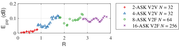
Some codes selected from Figs. 3 and 7 are shown in Fig. 8, whose resolution rates range from 0.15 to 3.83 in a step size $\leq 0.16$. This shows that we can approach the theoretic minimum energy per code symbol to within 0.13 dB across a wide range of resolution rates for up to 1024-QAM, using codebooks of a cardinality not larger than 256.

To achieve a fixed resolution rate $R_{\text{Frame}}<\log_{2}M$ in each fixed-length frame for the $M$-ASK alphabet, we use two different codes: a prefix-free code $\mathcal{C}_{1}:\bm{\mathcal{B}}_{1}\mapsto\bm{\mathcal{X}}_{1}$ with unequal codeword resolution rates, whose mean value $\mathsf{R}_{\mathcal{C}_{1}}$ is close to $R_{\text{Frame}}$, and a trivial code $\mathcal{C}_{2}:\bm{\mathcal{B}}_{2}\mapsto\bm{\mathcal{X}}_{2}$ with an equal codeword resolution rate $\mathsf{R}_{\mathcal{C}_{2}}=\log_{2}{M}>\mathsf{R}_{\mathcal{C}_{1}}$ across all the codewords (i.e., $\mathcal{C}_{2}$ is a typical F2F mapper for uniform $M$-ASK). The idea is that we begin encoding with $\mathcal{C}_{1}$ and then switch to $\mathcal{C}_{2}$ at some point of the successive encoding process if an overflow is predicted. If we keep counting the numbers of input bits and output symbols encoded by $\mathcal{C}_{1}$ in the first part of encoding, we can also calculate the number of symbols required to encode all the remaining input bits if we use $\mathcal{C}_{2}$ instead of $\mathcal{C}_{1}$ from that point onward, enabling prediction of an overflow. In what follows, we will show that this prediction can be made in a way that unique decoding is possible, and that the penalty due to this switching is small.

Let $k$ and $n$ be, respectively, a fixed number of input bits and a fixed number of output symbols of a PCDM encoder in each frame; i.e., the information bits and the code symbols belong to $\mathcal{B}^{k}$ and $\mathcal{X}^{n}$, respectively. Then, framing enables PCDM to achieve a fixed ${R}_{\text{Frame}}$, where

This shows that, for the chosen $\mathsf{R}_{\mathcal{C}_{1}}$ and $\mathsf{R}_{\mathcal{C}_{2}}$, an additional rate adaptability is also offered by framing, at the expense a larger energy gap. Let $\bm{b}^{(\ell)}$ and $\bm{x}^{(\ell)}$ denote the information word and the codeword chosen at the encoding iteration $\ell$ by $\mathcal{C}_{1}$, respectively. And assume that the use of $\mathcal{C}_{1}$ until iteration $\ell-1$ was assured not to cause an overflow, as long as we switch to $\mathcal{C}_{2}$ from the next iteration $\ell$ onwards. Hence we have used $\mathcal{C}_{1}$ until iteration $\ell-1$. Then, at the next iteration $\ell$, in order to foresee if $\mathcal{C}_{1}$ does not still cause an overflow, we need to ensure that

where $\gamma_{\text{Ava}}^{(\ell)}:=n-\sum_{i=1}^{\ell}l(\bm{x}^{(i)})$ is the number of available slots in the frame at the beginning of iteration $\ell+1$ and $\gamma_{\text{Req.}}^{(\ell)}:=\left\lceil(k-\sum_{i=1}^{\ell}l(\bm{b}^{(i)}))/{\mathsf{R}_{\mathcal{C}_{2}}}\right\rceil$ is the number of required symbol slots in case we switch to $\mathcal{C}_{2}$ at iteration $\ell+1$, respectively. Codebook $\mathcal{C}_{1}$ is used for encoding at iteration $\ell$ if condition (20) is fulfilled, otherwise $\mathcal{C}_{2}$ from iteration $\ell$ onwards. Notice that (20) can be evaluated only after seeing the incoming bits at iteration $\ell$ to obtain $l(\bm{b}^{(\ell)})$ and $l(\bm{x}^{(\ell)})$. This makes unique decoding impossible, since, assuming that unique decoding was successfully performed until iteration $\ell-1$ such that $l(\bm{b}^{(i)})$ and $l(\bm{x}^{(i)})$ are known for all $i=1,\ldots,\ell-1$, the decoder cannot identify which codebook was used at iteration $\ell$ without knowing $l(\bm{b}^{(\ell)})$ and $l(\bm{x}^{(\ell)})$. This suggests that, for unique decoding, the codebook used at iteration $\ell$ must be identified without relying on $l(\bm{b}^{(\ell)})$ and $l(\bm{x}^{(\ell)})$, which can be realized by a bounding technique. Namely, in a pessimistic assumption that the shortest information word is mapped to the longest codeword of $\mathcal{C}_{1}$ at iteration $\ell$, we can find the lower bound of the available slots and the upper bound of the required slots as

and

where $l_{\max}(\bm{\mathcal{X}}):=\max_{\bm{x}\in\bm{\mathcal{X}}}l(\bm{x})$ and $l_{\min}(\bm{\mathcal{B}}):=\max_{\bm{b}\in\bm{\mathcal{B}}}l(\bm{b})$. Now, without knowledge of $l(\bm{b}^{(\ell)})$ and $l(\bm{x}^{(\ell)})$, the condition (20) can be conservatively examined by

since $\gamma_{\text{Ava}}^{(\ell)}\geq\underline{\gamma}_{\text{Ava}}^{(\ell)}$ and $\overline{\gamma}_{\text{Req}}^{(\ell)}\geq\gamma_{\text{Req}}^{(\ell)}$.

References

- [1] G. Böcherer and R. A. Amjad, “Fixed-to-variable length resolution coding for target distributions,” in Proc. IEEE Inform. Theory Workshop, Sept 2013, pp. 1–5.
- [2] B. P. Tunstall, “Synthesis of noiseless compression codes,” Ph.D. dissertation, Georgia Institute of Technology, 1967.
- [3] B. Varn, “Optimal variable length codes (arbitrary symbol cost and equal code word probability),” Informa. Control, vol. 19, pp. 289–301, 1971.
- [4] T. C. Hu and A. C. Tucker, “Optimal computer search trees and variable-length alphabetical codes,” SIAM J. Applied Math., vol. 21, pp. 514–532, 1971.
- [5] G. D. Forney Jr., R. G. Gallager, G. R. Lang, F. M. Longstaff, and S. U. Qureshi, “Efficient moduiation for band-limited channels,” IEEE J. Select. Areas Commun., vol. SAC-2, no. 5, pp. 632–647, 1984.
- [6] A. R. Calderbank and L. H. Ozarow, “Nonequiprobable signaling on the Gaussian channel,” IEEE Trans. Inform. Theory, vol. 36, no. 4, pp. 726–740, 1990.
- [7] G. D. Forney Jr., “Trellis shaping,” IEEE Trans. Inform. Theory, vol. 38, no. 2, pp. 281–300, 1992.
- [8] J. N. Livingston, “Shaping using variable-size regions,” IEEE J. Select. Areas Commun., vol. 38, no. 4, pp. 1347–1353, 1992.
- [9] F. R. Kschischang and S. Pasupathy, “Optimal nonuniform signaling for Gaussian channels,” IEEE Trans. Inform. Theory, vol. 39, no. 3, pp. 913–929, 1993.
- [10] D. Raphaeli and A. Gurevitz, “Constellation shaping for pragmatic turbo-coded modulation with high spectral efficiency,” IEEE Trans. Commun., vol. 52, no. 3, pp. 341–345, 2004.
- [11] S. Kaimalettu, A. Thangaraj, M. Bloch, and S. W. McLaughlin, “Constellation shaping using LDPC codes,” in Proc. IEEE Int. Symp. Inform. Theory, 2007, pp. 2366–2370.
- [12] M. C. Valenti and X. Xiang, “Constellation shaping for bit-interleaved LDPC coded APSK,” IEEE Trans. Commun., vol. 60, no. 10, pp. 2960–2970, 2012.
- [13] G. Böcherer, F. Steiner, and P. Schulte, “Bandwidth efficient and rate-matched low-density parity-check coded modulation,” IEEE Trans. Commun., vol. 63, no. 12, pp. 4651–4665, 2015.
- [14] T. V. Ramabadran, “A coding scheme for m-out-of-n codes,” IEEE Trans. Commun., vol. 38, no. 8, pp. 1156–1163, 1990.
- [15] P. Schulte and G. Böcherer, “Constant composition distribution matching,” IEEE Trans. Inform. Theory, vol. 62, no. 1, pp. 430–434, 2016.
- [16] T. Fehenberger, D. S. Millar, T. Koike-Akino, K. Kojima, and K. Parsons, “Multiset-partition distribution matching,” January 2018. [Online]. Available: http://arxiv.org/abs/1801.08445
- [17] G. R. Lang and F. M. Longstaff, “A leech lattice modem,” IEEE J. Select. Areas Commun., vol. 7, no. 6, pp. 968–973, 1989.
- [18] R. Laroia, N. Farvardin, and S. A. Tretter, “On optimal shaping of multidimensional constellations,” IEEE Trans. Inform. Theory, vol. 40, no. 4, pp. 1044–1056, 1994.
- [19] P. Schulte and F. Steiner, “Shell mapping for distribution matching,” March 2018. [Online]. Available: http://arxiv.org/abs/1803.03614
- [20] Y. C. Gultekin, W. J. van Houtum, S. Serbetli, and F. M. . Willems, “Constellation shaping for IEEE 802.11,” in Proc. IEEE Annu. Int. Symp. Personal, Indoor, Mobile Radio Commun., 2017, pp. 1–7.
- [21] T. Yoshida, M. Karlsson, and E. Agrell, “Low-complexity variable-length output distribution matching with periodical distribution uniformalization,” in Proc. Opt. Fiber Commun. Conf., March 2018, pp. 1–3.
- [22] P. Schulte and B. C. Geiger, “Divergence scaling of fixed-length, binary-output, one-to-one distribution matching,” in Proc. IEEE Int. Symp. Inform. Theory, 2017, pp. 3075–3079.
- [23] J. Abrahams, “Variable-length unequal cost parsing and coding for shaping,” IEEE Trans. Inform. Theory, vol. 44, no. 4, pp. 1648–1650, 1998.
- [24] A. Lempel, S. Even, and M. Cohn, “An algorithm for optimal prefix parsing of a noiseless and memoryless channel,” IEEE Trans. Inform. Theory, vol. IT-19, pp. 208–214, 1973.
- [25] R. A. Amjad and G. Böcherer, “Fixed-to-variable length distribution matching,” in Proc. IEEE Int. Symp. Inform. Theory, 2013, pp. 1511–1515.
- [26] V. S.-N. Choi and M. Golin, Lopsided trees: Analyses, algorithms, and applications. Berlin, Heidelberg: Springer Berlin Heidelberg, 1996, pp. 538–549.
- [27] M. J. Golin and N. Young, “Prefix codes: Equiprobable words, unequal letter costs,” SIAM J. Comput., vol. 25, pp. 1281–1292, 1996.
- [28] M. J. Golin and G. Rote, “A dynamic programming algorithm for constructing optimal prefix-free codes with unequal letter costs,” IEEE Trans. Inform. Theory, vol. 44, no. 5, pp. 1770–1781, 1998.
- [29] M. J. Golin and J. Li, “More efficient algorithms and analyses for unequal letter cost prefix-free coding,” IEEE Trans. Inform. Theory, vol. 54, no. 8, pp. 3412–3424, 2008.
- [30] G. Böcherer and R. Mathar, “Matching dyadic distributions to channels,” in Proc. Data Compression Conf., 2011, pp. 23–32.
- [31] T. H. Cormen, C. Stein, R. L. Rivest, and C. E. Leiserson, Introduction to Algorithms, 2nd ed. McGraw-Hill Higher Education, 2001.
- [32] R. P. Stanley, Catalan Numbers. Cambridge University Press, 2015.
- [33] N. Dershowitz and S. Zaks, “Enumerations of ordered trees,” Discrete Math., vol. 31, no. 1, pp. 9–28, Jan. 1980.
- [34] T. M. Cover and J. A. Thomas, Elements of Information Theory 2nd Edition. Willey-Interscience, 2006.
- [35] CVX Research, Inc., “CVX: Matlab software for disciplined convex programming, version 2.1,” http://cvxr.com/cvx, Mar. 2017.
- [36] M. Grant and S. Boyd, “Graph implementations for nonsmooth convex programs,” in Recent Advances in Learning and Control. Springer-Verlag Limited, 2008, pp. 95–110.
- [37] S. Boyd and L. Vandenberghe, Convex Optimization. Cambridge University Press, 2004.
- [38] G. Böcherer, “Capacity-achieving probabilistic shaping for noisy and noiseless channels,” Ph.D. dissertation, RWTH Aachen University, 2012.
- [39] F. Jelinek, “Buffer overflow in variable length coding of fixed rate sources,” IEEE Trans. Inform. Theory, vol. 14, no. 3, pp. 490–501, May 1968.
- [40] R. A. Amjad, “Algorithms for simulation of discrete memoryless sources,” Master’s thesis, Technische Universität München, 2013.
- [41] P. J. Davis and P. Rabinowitz, Methods of numerical integration. Courier Corporation, 2007.
- [42] J. Cho and L. Schmalen, “Construction of protographs for large-girth structured LDPC convolutional codes,” in Proc. IEEE Int. Conf. Commun., 2015, pp. 4412–4417.
- [43] R. R. Müller, “Advanced modulation formats and signal processing for high speed spectrally efficient optical communications,” Ph.D. dissertation, Institut National des Télécommunications, 2016.
- [44] N. S. Muhammad, “Coding and modulation for spectral efficient transmission,” Ph.D. dissertation, University of Stuttgart, 2010.