Gaseous wakes and dynamical friction: mass-losing and mass-gaining perturbers
Abstract
An extended gravitational object embedded in a parent system comprised of gas and collisionless particles may undergo both dynamical friction (DF) and mass loss by tidal forces. If the object is compact enough, it can increase its mass through accretion of material from the surrounding medium. We extend the classical linear analysis of DF on a constant-mass body in a gaseous medium to the case where its mass changes with time. We show that the structure of the wake may differ significantly from the constant-mass case. For instance, the front-back symmetry of density about subsonic constant-mass perturbers is broken down for variable-mass perturbers. The density wake keeps a memory of the past mass history of the perturber. For dissolving perturbers, the density field is more dense than expected using the instantaneous mass of the perturber in the classical formula. As a consequence, the instantaneous-mass approximation underestimates the drag force for mass-losing perturbers and overestimates it for mass-gaining perturbers. We present cases in which the percentage error in the drag force using the instantaneous-mass approximation is greater than .
Keywords:
hydrodynamics – ISM: kinematics and dynamics – galaxies: star clusters – galaxies: evolution1 INTRODUCTION
A gravitational body moving through a field of light particles, or through a gaseous medium, experiences a drag force known as dynamical friction (DF), as a consequence of the continuous gravitational deflection of field particles or fluid elements (Chandrasekhar, 1943; Bondi & Hoyle, 1944). DF may induce an exchange of angular momentum between the massive object and the background particles, which leads to an orbital spiraling of the object towards the centre of the potential.
DF in a gaseous medium may be relevant to describe the orbital evolution of planetesimals or planets in eccentric or inclined orbits, when they are still embedded in the gaseous protoplanetary disc (Muto et al., 2011; Rein, 2012; Cantó et al., 2013; Xiang-Gruess & Papaloizou, 2013; Grishin & Perets, 2015). Common-envelope binary stars, or stars in gas-embedded star clusters may also suffer orbital decay due to gaseous DF (Ricker & Taam, 2008; Chavarría et al., 2010; Leigh et al., 2014). At subgalactic scales, gaseous DF is important during the early phases of galaxy evolution (Ostriker, 1999). It is also especially relevant in the central parts of gas-rich galaxies. Indeed, gaseous DF plays a key role in the orbital shrinking of supermassive binary black holes in the central parts of gas-rich mergers of galaxies. Globular clusters and nuclear star clusters may also suffer significant migration due to DF with the gas component in gas-rich dwarf galaxies (Antonini et al., 2012; Guillard et al., 2016, e.g.,).
Most estimates of the DF force assume that the body is on a straight-line trajectory at constant velocity through a homogeneous gaseous medium (Bondi & Hoyle, 1944; Dokuchaev, 1964; Ruderman & Spiegel, 1971; Bisnovatyi-Kogan et al., 1979; Rephaeli & Salpeter, 1980; Ostriker, 1999; Edgar, 2004; Cantó et al., 2013, e.g.,) In recent years, the DF force has been studied adding other physical phenomena or adopting different assumptions. Kim & Kim (2007) computed the density wake and the DF on perturbers in circular orbits. Sánchez-Salcedo & Chametla (2014) investigated the drag force on a binary system and the torques on each component of the binary. The DF force on a perturber travelling in a magnetized gas has been studied in Sánchez-Salcedo (2012) and Shadmehri & Khajenabi (2012). Namouni (2010) relaxed the assumption that the body moves at constant velocity and derived the DF on decelerating perturbers. On the other hand, Lee & Stahler (2011) showed that, for subsonic perturbers, the drag force magnitude depends on whether the perturber can accrete mass or not.
In all the abovementioned studies, it is generally assumed that the perturber has constant mass. However, in many scenarios, astrophysical bodies may lose or gain material and thereby its mass changes. For instance, planets embedded in protoplanetary discs, may undergo rapid mass accretion at a rate that can be understood in terms of accretion within the Bondi radius or within the Hill radius, depending on its mass (D’Angelo & Lubow, 2008, e.g.,). On the other hand, in star-forming molecular clouds, high-mass stars may form due to continued accretion of gas funneling to the centre of the cluster potential (Bonnell & Bate, 2006). The mass function of star clusters may also indicate that clusters also grow by accretion (Kuznetsova et al., 2017).
Extended objects, such as star clusters and satellite galaxies, can lose mass due to stripping by the tidal field of the host galaxy or by ram pressure. Especially dwarf galaxies may experience rapid mass loss when stellar feedback blows out a large fraction of gas (Governato et al., 2010). As quantitatively described by Zhao (2004), the strength of the tidal forces on satellite galaxies and star clusters increase as they sink towards the galactic centre due to DF. On some occasions, tidal forces may lead to a complete disruption of the stellar cluster or satellite. According to the CDM models of Fattahi et al. (2018), some dwarf spheroidal galaxies in the haloes of the Milky Way and Andromeda have been very heavily stripped. For instance, the fraction of mass lost in Crater 2 and Andromeda XIX is about percent.
Since the strength of the DF force depends on the mass of the perturber (or satellite), the DF timescale, that is the time to reach the host’s centre from a certain initial radius, depends not only on the initial mass of the perturber, but also on the mass loss rate (Colpi et al., 1999; Gan et al., 2010, e.g.,). As a first approximation, one should use the instantaneous bound mass of the perturber to estimate the DF force. However, the mass in the tidal debris may also affect DF: stripped material that remains in the vicinity of the perturber also contributes to the DF because they gravitationally interact with the bound stars (Fujii et al., 2006; Fellhauer & Lin, 2007). This material also disperses background particles and enhances the amplitude of the wake behind the perturber. These tidal debris effects are important for stellar systems undergoing tidal disruption (Fellhauer & Lin, 2007, e.g.,).
In this work we study a different aspect of the DF force acting on a body of changing mass. Our analysis pivots on the fact that the wake excited in ambient medium keeps a memory of the history of the mass of the perturber. Since the drag force arises from the gravitational attraction between the body and its induced wake, the drag force should also reflect the history dependent nature of the wake. Our aim is to estimate the DF on a variable-mass perturber as well as to quantify how much it differs from the drag force derived using the instantaneous mass of the perturber.
The paper is organized as follows. In Section 2, we describe the linear hydrodynamical approach to derive the gaseous wake in the medium and the DF force. In Section 3, we describe the structure of the wake induced by a body with non-constant, continuously varying mass. Computations of the DF force are given in Section 4. Finally, we give a brief discussion and the conclusions in Section 5.
2 Gravitational wakes: basics and model
2.1 Variable-mass perturber
We consider a gravitational body moving through a gaseous medium. The gas will respond to the gravitational pull created by this object. The perturber’s gravitational potential, , satisfies the Poisson equation:
| (1) |
where is the density profile of the perturber. The temporal evolution of depends on how the process of mass gain and/or mass stripping occurs. For simplicity, we assume that the shape of the density profile of the perturber does not change with time, so that the perturber’s profile factorizes as
| (2) |
where is the position of the centre of mass of the perturber. If is taken as a constant value, then we recover the constant-mass case. The mass that remains bound to, or in the vicinity of the pertuber, is
| (3) |
where is a constant with dimensions of mass. Thus, the mass of the perturber changes at a rate given by .
To quantify the DF force, we adopt a rather generic function for . We will assume that the perturber is formed at (where ), then it evolves at constant mass in the interval . At , it starts a phase of exponential mass loss or mass gain with a characteristic timescale . Such a situation can be described by the function
| (4) |
with . A mass model is specified by four parameters: , , and . Here is the fraction of mass that the perturber has lost or gained since to . More specifically, the mass of the perturber is at , and it is at . Values in the range correspond to mass loss. For models with , the perturber enhances its mass. In a more compact notation, can be written as
| (5) |
where is the Heaviside function. If we adopt or , it describes a case where the perturber is turned on at and remains with constant mass at later times. This case was studied by Ostriker (1999).

Figure 1 shows a sketch of four representative models. The meaning of depends on the setting and configuration of the system under study. For instance, if we are interested in studying the DF on a forming object as that depicted in the third panel of Figure 1, we may choose . In other astrophysical settings, may represent the time elapsed since the body has entered into the gas medium until it experiences mass loss. In fact, tidal forces do not lead to significant mass stripping if the size of the body is smaller than the tidal radius. Once the tidal radius has been filled due to tidal heating, the satellite may suffer important tidal stripping.
A period of almost constant mass and a subsequent episode of mass loss, as the scenario shown in the first panel of Figure 1, are easily recognizable in simulations of tidal evolution of satellite systems; tidal effects are more intense at pericentre passages, where episodes of severe mass loss occur (Peñarrubia et al., 2010, e.g.,). We will return to the discussion of the physical meaning of in §5.
Although our choice of gives enough leeway to explore the significance of different parameters, other variants may be also relevant. For instance, collisional -body calculations of isolated star clusters show an almost linear decrease of mass with time (Baumgardt, 2001). In Appendix D, more generic choices for the mass evolution of the perturber are considered.
2.2 Linear equations and formal solution
To derive the density structure of the wake induced by the perturber, we will follow the same approach as described in Ostriker (1999). The unperturbed gaseous medium is homogenous and infinite, with density and sound speed . The gas is initially at rest. Far enough from the perturber, the disturbances in gas density and velocity are always linear. Close to the perturber, the perturbations might be also linear if the characteristic size of the perturber is much larger than the accretion radius defined as , where is the velocity of the perturber (see §3).
We define the perturbed gas density as and the perturbed gas velocity as . Provided that and , the linearized Euler equations describe the evolution of the system. In terms of and they can be written as
| (6) |
| (7) |
By combining these two equations, it is simple to show that satisfies the following inhomogeneous wave equation
| (8) |
The solution to this equation is
| (9) |
Once is specified, we may compute . In our case and according to Equations (2) and (5), is the sum of three terms
| (10) |
with
| (11) |
| (12) |
| (13) |
Since Equation (9) is linear, the perturbed density is a superposition of each individual solution. More specifically, if is the perturbed density created by a perturber with a density profile , then . For shortness, we will refer to the wake associated with the mass density term as the wake 1, and so on.
Once is computed, the gravitational drag felt by the perturber is given by
| (14) |
As usual, the integral is performed over all volume excluding a sphere of radius around the perturber, where is the distance from the perturber at which the linear approximation breaks down.
2.3 Particular case: Constant-mass perturber
Dokuchaev (1964), Ruderman & Spiegel (1971) and Rephaeli & Salpeter (1980) calculated, in linear theory, the density structure of the stationary wake induced by a gravitational object of constant mass , moving in a rectilinear orbit with velocity . The stationary case corresponds to in our notation. The gas response depends on the Mach number of the perturber, defined as . In the stationary wake, subsonic perturbers generate density distributions whose isodensity contours are ellipsoids centred on the perturber. Therefore, the net DF force on subsonic perturbers is zero in the steady-state flow. For supersonic bodies, the magnitude of the DF force is given by
| (15) |
where is the Coulomb logarithm. Here and are the minimum and maximum radii of the effective gravitational interaction of a perturber with a gas.
Ostriker (1999) performed the time-dependent analysis of the wake produced by a perturber that is turned on at (Just & Kegel, 1990, see also). She found that the perturbed density in the wake is
| (16) |
where , with the cylindrical radius, and
| (17) |
Ostriker (1999) noticed that the finite-time perturbation is more appealing because it captures more relevant physics than the stationary approach. For instance, she showed that the DF force is nonzero even for subsonic perturbers. The magnitude of the force for subsonic perturbers is given by Equation (15) with
| (18) |
provided that . In addition, the time-dependent analysis allows to remove the ambiguity in the definition of and permits to find the temporal behaviour of the Coulomb logarithm. For supersonic perturbers and at , she found
| (19) |

3 The structure of the wake
In the following, we present the density structure of the wake induced by a perturber whose mass varies over time according to Equations (2) and (5). We assume that the perturber moves at constant velocity in a rectilinear orbit along the -axis. The position of the centre of mass of the body is and its density can be written as
| (20) |
In Appendix A and B, we evaluate the integral given in Equation (9) to obtain the analytical expressions for the three components of the wake (, and ) excited by a point-mass perturber . The reliability of our analyical derivation of has been proven by comparing with the results of hydrodynamical simulations (see Appendix C).
The wakes and are Ostriker type wakes; corresponds to the wake created by a perturber of mass formed at , and is the wake created by a fictitious perturber of mass formed at (wake 2). The solution for is:
| (21) |
Since the analysis is linear, the above expression for is only valid at those values of for which . The values for and are given in Appendix A, whereas can be found in Equation (73). The functions , and depend on the position and time , as well as on the parameters , and . As shown in the Appendices A and B, the functions , and , take values between and .
In a scenario where the perturber dissolves, it is natural to assume that the perturber is extended. If the characteristic physical size of the perturber is larger than , the response of the gas is linear at any position in space (Bernal & Sánchez-Salcedo, 2013, e.g.,). In that case, the perturbed density induced by a softened perturber, , can be calculated using the convolution theorem as
| (22) |
where is given in Equation (21). Nevertheless, the perturbed density and velocity in the far field (at distances much larger than the size of the perturber) are essentially the same for extended and point-mass perturbers.

Figure 2 shows colour maps of the perturbed density at time , for different combinations of and . In all the four cases, . Hence the current mass of the perturber is and for and , respectively. We see that the wake structure is more complex than in the standard case . As said in §2.3, the isodensity contours for subsonic constant-mass perturbers are ellipsoids. However, as the model with and illustrates, the contours are not longer ellipsoids; some isodensity contours are flattened along the line of motion of the perturber but others do not. Interestingly, the backward-forward symmetry of the wake excited by constant-mass subsonic perturbers, is broken down for varying-mass perturbers (see also the map for the model with and ). On the other hand, for supersonic perturbers (), the density wake is confined to the Mach cone and sonic sphere, as occurs in the constant-mass case, but the isodensity contours are not longer hyperbolae.
In order to quantify the imprint of time-dependent mass on the structure of the wake, we compare with , defined as the perturbed density derived in the constant-mass approximation. More specifically, is the perturbed density simply adapting Ostriker’s formula for a body created at , and taking the mass of the perturber as the instantaneous mass :
| (23) |
Recall that the wake factor is analogous to , but for a body formed at .
At , it holds that . However, at , the difference between the exact value for the perturbed density , and the value derived in the instantaneous approximation is
| (24) |
Therefore, the fractional change of the density relative to is
| (25) |
In regions where is different from zero, the wake keeps a memory of the past mass of the perturber.
Figure 3 shows for different combinations of parameters. It is a generic result that when the perturber dissolves (i.e. ), at any point in space because ; the vake is more dense than predicted in the instantaneous approximation because the perturber was more massive in the past. Conversely, when the perturber gains mass (), everywhere. In this case, the wake is less dense than .
For subsonic perturbers, is larger in the outer parts of the wake than in the inner parts. In fact, decreases close to the body (see Fig. 3). For supersonic perturbers, is also larger in the outer parts of the wake that are far away from the body than in the near field region, but it does not drop monotonically when we approach from the outer wake towards the perturber; exhibits a jump when we cross the sonic sphere.
By comparing the panels at and at in Figure 3, we see that, as time goes by, the volume around the body having low values of becomes increasingly larger. At larger times and for the subsonic case, asymptotically approaches to zero, i.e. the wake loses memory of the mass history, except in a very narrow region in the very outer parts of the sonic sphere. For supersonic perturbers, decreases with time in most parts of the wake, both in the sonic sphere and within the Mach cone. In the limit , decreases at any point because of the geometrical dilution of the sound waves launched by the perturber when it had a different mass. However, it is interesting to note that even at , when the perturber has almost reached its final mass, in a significant portion of the wake for the case , either if the body moves subsonically or supersonically.
Given , , and , the shape of the contours of does not depend on the value of (see Figure 3). The reason is that the functions , and , which determine the shape of the contours, do not depend on 11 1 Consider two models A and B with the same parameters , and but different . For illustration, suppose that model A has and model B has . We obtain at , and at ..
4 Dynamical friction force
In this Section, the gravitational tug on the perturber by the overdense wake is calculated using Equation (14). For a perturber in rectilinear orbit with velocity and , the gravitational drag can be recast in terms of and as
| (26) |
We expect that slows down the perturber even if the mass of the perturber varies over time. Consequently, if we write , we expect that .
At , the mass of the perturber is constant and, therefore, the drag force is given in Ostriker (1999):
| (27) |
where is given by Equation (18) for subsonic perturbers, and
| (28) |
for supersonic perturbers (). These expressions for are valid for .
In the following, we wish to quantify at , that is, when the episode of mass loss or mass gain has started. Since the linear analysis for a point-mass wake is only valid at (see Appendix A and Ostriker 1999), we will focus on estimating at .
To make comparisons, it is convenient to define as the strength of the DF force using the instantaneous mass approximation, i.e. by assuming that the wake behind the perturber has density . More specifically, is given by Equation (27), but replacing for . So,
| (29) |
with
| (30) |
is given by Equation (18) for subsonic perturbers, and by Equation (28) for supersonic perturbers.
We wish to determine how much the DF force deviates from . To do so, we combine Equations (3), (24) and (26) to find that
| (31) |
where the second term , which we will refer to it as the memory term, is given by
| (32) |
where
| (33) |
and
| (34) |
| (35) |
The integral in can be performed analytically to obtain
| (36) |
The two-dimensional integral is much more complicated and will be computed numerically.
From Equation (36), it is obvious that if (indeed in this case). In the general case, we have . On the other hand, even though may be positive or negative, we anticipate that is always positive or zero, and therefore is positive or negative depending on the sign of . The memory term is positive when the perturber loses mass () because the wake is more dense than (see §3). Therefore, underestimates the drag force in this case. If the perturber gains mass, the memory term is negative, and overestimates the drag force.
For constant-mass perturbers (either for or for ), the memory term must be zero. In fact, if , it holds from Equation (32) that and hence . On the other hand, if , Eq. (33) implies . Moreover, (see Appendix B) and according to Eqs. (32), (34) and (35), .
is expected to be different from if the perturber had a different mass in the past. In the following, we study how depends on the mass history of the perturber and on time. Before dealing with the general case, we examine a scenario where , which corresponds to a very rapid change of mass, in the next subsection.
4.1 Dynamical friction for the case
The case describes a situation where the perturber undergoes an instantaneous boost in mass at . Assuming that , the perturber’s mass changes from to . From Equations (4) and (33) we have that , and at . Therefore, from Eqs. (32) and (36), the memory term is given by
| (37) |
with
| (38) |
Hence as . One can show that , implying that the net DF force is always opposed to the motion of the perturber.

According to Eq. (37), if . This implies that the DF force on a subsonic perturber with is identical to the DF force felt by a perturber with constant mass since its birth.
For supersonic perturbers, at , the memory term in nonzero, except for . Interestingly, does not depend on . It does depend on but just through the factor . If (and ), gives the correct value of the force because the perturber has constant mass.
It is worthwhile to compare with . For supersonic bodies, we find that
| (39) |
where is given in Equation (28). The instantaneous mass approximation is satisfactory if is small. In order to show the dependence of on time, we consider cases where the length of the wake at is much larger than . Since the length of the wake at is , we will focus on cases where . Figure 4 shows (which it is just ) as a function of time for and two different values of . We see that decreases with time, and their values are rather insensitive to the Mach number of the perturber. At a given , is larger for low values of . At , underestimates the drag force by a factor of .
For any arbitrary , the average value of between and , is for , whereas it is for . Note that depends on the value of as follows .
Under our assumption here that , values for more negative than are not very realistic because the remnant would become gravitationally unbound and completely disrupted in a short timescale. For , is a sizeable fraction of on a characteristic timescale .
4.2 Dynamical friction for the case
In this subsection, we obtain for models with . In this general case, we need to compute . This term takes into account the contribution of the wake (see Equation 35).

4.2.1 Subsonic perturbers
According to Eq. (36), for subsonic perturbers. Thus,
| (40) |
is obtained by integrating numerically Equation (35). We find that remains constant over time for subsonic perturbers. More specifically, in the subsonic case, only depends on two dimensionless parameters and , which is defined as , i.e.
| (41) |
Note that depends neither on nor on in the subsonic case.
Figure 5 shows as a function of , for different values of . The values of are positive. For a fixed value of , increases steeply with . On the other hand, for a given , the function and thereby decrease with . In the following, we estimate the contribution of to the drag force in order to find the values of for which the instantaneous approximation could be adequate.
At , the following inequality holds for any value of
| (42) |
On the other hand, we have that . Therefore, the ratio of to is at most. In Figure 5, we can compare with . We see that for and , is a factor larger than . Therefore, for those values of and , the instantaneous approximation has a percentage error of at most for perturbers with .
Consider now the case . The relative contribution of to the drag force increases with . This is exemplified in Figure 6, which shows for and two different values of . For point-mass perturbers and for the values of explored in Figure 6 (namely, ), overestimates the drag force by less than , even for . We warn that this claim is valid at , because linear theory cannot predict the drag force in the interval , for point-mass perturbers. It is worth noting that in terms of and is
| (43) |
Therefore, for , linear theory cannot predict the drag force in a time interval .
For softened perturbers, however, the response is linear at any location if the softening radius is large compared to the accretion radius. In this case, can be calculated at any time using given in Equation (22). In the bottom panel of Figure 6, we plot for a Plummer perturber with radius and moving at Mach number . Here denotes the drag force using for a softened Plummer perturber. For a fair comparison between point-mass and extended perturbers, we have used for Plummer perturbers instead of (Sánchez-Salcedo & Brandenburg, 1999; Bernal & Sánchez-Salcedo, 2013, see).

In Figure 6 we see that reaches a maximum and then declines with time, approaching asymptotically. For , and , the mean value of between and is , whereas it is for and . For , and , the above average value is less than (i.e., overestimates the true drag force by or less).

The result that depends on implies that if we wish to know the temporal evolution of , we need to know how the mass is added to the perturber. For instance, if a Plummer body grows in mass keeping constant its central density, its radius should increase over time according to the law . As a consequence, declines with time. This will result in a more rapid drop of over time. This effect will be more notorious for large values of .
The rate of change of the velocity of the perturber is . The classical Ostriker formula can be used to estimate this frictional deceleration if the mass of the perturber is formally replaced by an effective mass . By definition, satisfies the relationship
| (44) |
Figure 7 plots the effective mass for models with and . For positive , the effective mass is always smaller than the instantaneous mass. We see that for the model with , the effective mass at equals the perturber’s mass at (dashed line). In fact, the curves of the effective mass with time are less steep than the curve for the instantaneous mass.

4.2.2 Supersonic perturbers
In this subsection we consider bodies in supersonic motion . Combining Equations (33) and (36), we find
| (45) |
In the limit , the second term in the right-hand-side of Equation (45) can be neglected, and we recover the case discussed in Section 4.1.
In the following, we take , unless metioned otherwise. The function depends on four dimensionless parameters: and . Recall that was defined in Section 4.1 as . The value of can be found analytically in the limit and it is given by
| (46) |
Note that in this limit.
Figure 8 shows and versus time for and . For these values of and , . We have used that can be recast in terms of and as
| (47) |
Both and achieve a maximum and then decrease with time, approaching to zero at large . The curves with and reach the maximum at , outside the range displayed in Figure 8. The peak value of decreases as increases. For instance, the maximum value of is for , whereas it is for .

From the top panel of Figure 8, we see that , which implies that as the bottom panel shows. Thereby is positive if , and it is negative if (see Equation 32).
Figure 9 shows for , varying and . It is seen that depends weakly on and ; changing by a factor of and by a factor of , varies less than . For , this variation is less than (not shown). This implies that the precise values of and are not crucial to estimating . Indeed, we find that when is given, is rather insensitive to and , provided they lie in the range and . For this reason, we will focus our discussion on the case and , but all the results are also valid in the abovementioned range of and .

In order to quantify how much departs from the true drag force , Figure 10 displays for some representative cases, using and . Let us focus first on the case . For , decreases rapidly and continuously with time, approaching . At , it is larger than , implying that underestimates the drag force by a factor larger than . For (and ), rises from to , where it reaches a maximum and then declines. It is larger than between and . Finally, for , gradually increases along the time interval displayed in Figure 10, but it is always below .

In the interval , the average value of is , and for , and , respectively. In the interval , the average values are , and , respectively. It is remarkable that for a perturber with , having almost reached its final mass at , the true drag force is still as large as at .
For , the curves versus time behave rather similar to , but with less amplitude. For instance, for , is always less than . In other words, contributes to the drag force or less. For , contributes less than .
For mass-gaining objects with , the average values of between and are , and for , and , respectively. At , overpredicts by or less, even for . In particular, at , . If we compare the curves for with those for (in both cases the mass of the perturber changes by a factor of ), we find that the memory effect is longer-lasting for .
The effective mass for some of these models is shown in Figure 11. The offset between and is due to the history dependent nature of the process. As a consequence, the effective mass always takes a value between and .
Figure 12 shows a diagram in the (, ) plane, which outlines the parameter space where predicts correctly the value of the drag force within a factor of at any time. To build the plot, we use and . For instance, for , the error made by using is less than if . Since the curve is very stiff at , we require to have the same error for . Still, for and , the error is less than . On the other hand, for positive values of , the condition is much more stringent than the condition . For and , overestimates by a factor less than at any time.
For completeness, Figure 13 compares with for and . For in the range , they never differ from one another by a factor greater than .


5 Summary and final remarks
We have studied the gravitational response of a gaseous medium to the gravitational pull exerted by a body of time-varying mass. To model this, we examine a scenario where the perturber has constant mass during a lapse of time , and immediately thereafter it undergoes an episode of gain or loss of mass with a characteristic timescale . We have assumed that the body moves in rectilinear orbit through an initially homogeneous medium The main goals were to characterize the density perturbation in the gas and to calculate how the DF force depends on the mass history of the perturber. Our main results can be summarized as follows:
(i) The structure of the wake contains a record of the history of mass of the perturber. For perturbers that lose mass, the wake is more dense than predicted using the instantaneous mass in the classical Ostriker’s formula, especially in the outer parts of the wake, because the perturber was more massive in the past and thereby induced a stronger perturbation in the gas. If the perturber gains mass, the wake is less dense than predicted in the instantaneous approximation.
(ii) We have presented cases where large regions of the wake still retain memory of the past mass of the perturber even after a time , i.e. well after the episode of mass change has been completed.
(iii) No matter the perturber mass history, the net DF force is always opposed to the perturber’s velocity.
(iv) The DF force can be split into two components: the force predicted in the instantaneous approximation , plus a memory term. The memory term is positive, i.e. it contributes to the drag force, if the perturber loses mass. It is negative if the perturber increases its mass.
(v) The standard formulas for the rate of change of the perturber’s velocity can be applied once the mass of the perturber is replaced with an effective mass. We have shown that the effective mass is larger (smaller) than the instantaneous mass if the body loses (gains) mass.
The response of the gas depends on whether the body moves subsonically or supersonically. For subsonic perturbers of varying mass, we have found that
(i) The isodensity contours are not longer ellipsoids, and the well-known front-back symmetry of the density about constant-mass subsonic perturbers is broken down when the perturber’s mass is not constant.
(ii) The memory term vanishes if the change in mass occurs instantly (), implying that accurately gives the DF force. If the change of mass occurs during a non-vanishing time interval, the relative contribution of the memory term increases with increasing Mach number.
(iii) We have provided examples of mass-gaining perturbers in which overestimates the drag force by more than on the interval between and , i.e. throughout the episode of mass loss/gain.
For perturbers moving supersonically, we have found that
(i) The two critical parameters that determine the importance of the memory term are the fractional change of mass and the value of relative to . The relative difference between and reduces as the ratio increases.
(ii) For instant gain or loss of mass (), the memory term is initially large and then decreases with time to zero. For , the memory term acquires its maximum value at .
(iii) As a rule-of-thumb, gives the drag force with a percent error less than as long as the perturber’s mass changes by less than and .
Our results should find application in a number of astrophysical settings, such as the motion of dissolving systems (stellar clusters, globular clusters or dwarf satellite galaxies), through interstellar gas of the parent galaxy. Episodes of mass loss on short timescales may occur at pericentre passages or at late stages of tidal disruption.
It is also worth mentioning that the e-folding timescale for mass growth of stars and black holes embedded in a typical interstellar cloud or nuclear disks, through Bondi-Hoyle-Lyttleton accretion, is much longer than the orbital timescale. Under these circumstances and based on our results, the instantaneous approximation should be satisfactory. In star-forming molecular clouds, however, massive stars may form by competitive accretion in a timescale of the order of the free-fall time (Bonnell & Bate, 2006, e.g.,). Nevertheless, the assumption that the unperturbed medium is homogeneous and at rest is not strictly applicable due to the chaotic and turbulent nature of the environment.
In this work, we have considered only the gravitational drag exerted on the perturber from the density enhancement in the wake. In the case of a body that gains mass, it can also experience an aerodynamic drag due to the direct transfer of momentum by accreting material. For supersonic perturbers, the aerodynamic drag could be even more important than the dynamical drag.
We have adopted some idealized assumptions to explore the DF acting on perturbers of non-constant mass. In particular, we have assumed that the perturber moves in rectilinear orbit. In real systems, however, the orbit has some curvature. For constant-mass supersonic perturbers on an orbit with a typical size , the curvature of the orbit causes that the maximum impact parameter will cease to increase linearly with time. For perturbers with , the bending of the wake along the orbit leads to a cut-off in the impact parameter above (Sánchez-Salcedo & Brandenburg, 2001; Kim & Kim, 2007; Just et al., 2011). In this context, the time can be related to the orbital parameters by equating and, therefore, should be identified with the orbital timescale . On the other hand, because of the curvature of the orbit, the wake “restarts” over each one-quarter orbit. This leads to a reduction of the memory term at times relative to the rectilinear orbit. Therefore, the estimates of the memory term derived in the straight-line orbit should be considered as upper limits at . The above reasoning is only valid if . If this condition is not fulfilled, the gravitational pull of the wake ahead of the perturber cannot be ignored (Sánchez-Salcedo et al., 2018, e.g.,), and a more delicate analysis is required.
Acknowledgments
We thank the referee for constructive criticisms and valuable comments. We also thank Ana Hidalgo for useful input. The authors acknowledge funding from PAPIIT project IN111118.
References
- Antonini et al. (2012) Antonini F., Capuzzo-Dolcetta R., Mastrobuono-Battisti A., Merrit D. 2012, ApJ, 750, 111
- Baumgardt (2001) Baumgardt H. 2001, MNRAS, 325, 1323
- Bernal & Sánchez-Salcedo (2013) Bernal C. G., Sánchez-Salcedo F. J. 2013, ApJ, 775, 72
- Bisnovatyi-Kogan et al. (1979) Bisnovatyi-Kogan G. S., Kazhdan Ya. M., Klypin A. A., Lutskii A. E., Shakura N. I., 1979, SvA, 23, 201
- Bondi & Hoyle (1944) Bondi H., Hoyle F. 1944, MNRAS, 104, 273
- Bonnell & Bate (2006) Bonnell I. A., Bate M. R. 2006, MNRAS, 370, 488
- Cantó et al. (2013) Cantó J., Esquivel A., Sánchez-Salcedo F. J., Raga A. C. 2013, ApJ, 762, 21
- Chandrasekhar (1943) Chandrasekhar S. 1943, ApJ, 97, 255
- Chavarría et al. (2010) Chavarría L., Mardones D., Garay G., et al. 2010, ApJ, 710, 583
- Colpi et al. (1999) Colpi M., Mayer L., Governato F. 1999, ApJ, 525, 720
- D’Angelo & Lubow (2008) D’Angelo G., Lubow S. H. 2008, ApJ, 685, 560
- Dokuchaev (1964) Dokuchaev V. P. 1964, Soviet Astron., 8, 23
- Edgar (2004) Edgar R. 2004, New Astron. Rev., 48, 843
- Fattahi et al. (2018) Fattahi A., Navarro J. F., Frenk C. S., Oman K. A., Sawala T., Schaller M. 2018, MNRAS, 476, 3816
- Fellhauer & Lin (2007) Fellhauer M., Lin D. N. C. 2007, MNRAS, 375, 604
- Fujii et al. (2006) Fujii M., Funato Y., Makino J. 2006, PASJ, 58, 743
- Gan et al. (2010) Gan J.-L., Kang X., Hou J.-L., Chang R.-X. 2010, RAA, 10, 1242
- Governato et al. (2010) Governato F., et al. 2010, Nature, 463, 203
- Grishin & Perets (2015) Grishin E., Perets H. B. 2015, ApJ, 811, 54
- Guillard et al. (2016) Guillard N., Emsellem E., Renaud F. 2016, MNRAS, 461, 3620
- Just & Kegel (1990) Just A., Kegel W. H. 1990, A&A, 232, 447
- Just et al. (2011) Just A., Khan F. M., Berzcik P., Ernst A., Spurzem R. 2011, MNRAS, 411, 653
- Kim & Kim (2007) Kim H., Kim W.-T. 2007, ApJ, 665, 432
- Kuznetsova et al. (2017) Kuznetsova A., Hartmann L., Burkert A. 2017, ApJ, 836, 190
- Lee & Stahler (2011) Lee A. T., Stahler S. W. 2011, MNRAS, 416, 3177
- Leigh et al. (2014) Leigh N. W. C., Mastrobuono-Battisti A., Perets H. N., Boker T. 2014, MNRAS, 441, 919
- Muto et al. (2011) Muto T., Takeuchi T., Ida S. 2011, ApJ, 737, 37
- Namouni (2010) Namouni F. 2010, MNRAS, 401, 319
- Ostriker (1999) Ostriker E. C. 1999, ApJ, 513, 252
- Peñarrubia et al. (2010) Peñarrubia J., Benson A. J., Walker M. G., Gilmore G., McConnachie A. W., Mayer L. 2010, MNRAS, 406, 1290
- Rein (2012) Rein H. 2012, MNRAS, 422, 3611
- Rephaeli & Salpeter (1980) Rephaeli Y., Salpeter E. E. 1980, ApJ, 240, 20
- Ricker & Taam (2008) Ricker P. M., Taam R. R. 2008, ApJ, 672, L41
- Ruderman & Spiegel (1971) Ruderman M. A., Spiegel E. A. 1971, ApJ, 165, 1
- Sánchez-Salcedo (2012) Sánchez-Salcedo F. J., 2012, ApJ, 745, 135
- Sánchez-Salcedo & Brandenburg (1999) Sánchez-Salcedo F. J., Brandenburg A. 1999, ApJ, 522, L35
- Sánchez-Salcedo & Brandenburg (2001) Sánchez-Salcedo F. J., Brandenburg A. 2001, MNRAS, 322, 67
- Sánchez-Salcedo & Chametla (2014) Sánchez-Salcedo F. J., Chametla R. O. 2014, ApJ, 794, 167
- Sánchez-Salcedo et al. (2018) Sánchez-Salcedo F. J., Chametla R. O., Santillán A. 2018, ApJ, 860, 129
- Shadmehri & Khajenabi (2012) Shadmehri M., Khajenabi F. 2012, MNRAS, 424, 919
- Stone & Norman (1992) Stone J. M., Norman M. L. 1992, ApJS, 80, 753
- Xiang-Gruess & Papaloizou (2013) Xiang-Gruess M., Papaloizou J. C. B. 2013, MNRAS, 431, 1320
- Zhao (2004) Zhao H.S. 2004, MNRAS, 351, 891
Appendix A Perturbed density profiles for wakes and
In Section 2.2, we define as the wake produced by a perturber with a density profile
| (48) |
On the other hand, is the density perturbation in the wake induced by a body with a density distribution
| (49) |
It is straightforward to obtain and from Ostriker (1999). In the case of , the perturber is turned on at the location . At time , it holds . Now consider . We define Region 1 as the sonic sphere centred at :
| (50) |
For subsonic perturbers, the wake is confined to Region 1. For supersonic perturbers, we define Region 1′ as the rear Mach cone, which is the volume that satisfies the following conditions:
| (51) |
| (52) |
and
| (53) |
At , the associated density wake takes the form
| (54) |
where in Region 1, in Region 1′ only if , and otherwise.

The perturbed density is zero at . At , it is
| (55) |
where in Region , which is defined as the following sonic sphere
| (56) |
For supersonic perturbers (), in Region , which is specified by these three inequalities
| (57) |
| (58) |
and
| (59) |
Outside regions and , the medium remains unperturbed and, consequently, . A representative diagram of the Regions , , and is shown in Figure 14 for both subsonic and supersonic perturbers.
We recall that the above expressions for and are valid only for .
Appendix B Perturbed density for wake
As said in Section 2.2, denotes the density wake excited by a fictitious perturber with the following mass density:
| (60) |
At , is obtained from Equation (9). After performing the integration over , and , which are trivial, only the integral over is left. Using the variable instead of yields
| (61) |
To evaluate this integral, we find the two simple zeros, and , of the argument of the delta function:
| (62) |
and apply the identity that
| (63) |
where are the simple roots of .
As occurs in the derivation of by a constant-mass perturber (Ostriker, 1999), only the root is valid if . In fact, is not a valid root if because it does not satisfy the equality . Therefore, if , we have that
| (64) |
Given that is positive only if (i.e. in Region ), we find that
| (65) |
in Region , and it is zero outside region , provided that .
On the other hand, if , both and are valid in the region . Therefore, for ,
| (66) |
if , while otherwise.
Now consider the argument of the Heaviside function in Equation (66). In Region (and for ), it is easy to show that and and, therefore, and both terms in the sum in the RHS of Equation (66) are nonzero. More specifically, the perturbed density of the wake in Region is given by
| (67) |
In Region (and for ), and and therefore only the root contributes to the sum in Equation (66). In this region,
| (68) |
Putting all the results in a single form, the perturbed density at , for both subsonic and supersonic perturbers, is
| (69) |
where
| (70) |
and and . Note that . We see that when , then both and . Therefore, in Region 2 and in Region 2′, and the constant-mass case is recovered.
In contrast to and , which are bound quantities ( and are less than or equal to ), is not bound. However, algebraic calculations show that the factor , which appears in Equation (69), can only take values between and in Region 2, and between and in Region 2′. In the following, we outline how to find the extreme values of the function in the different regions.
Suppose that . The maxima of occur at locations where are also maxima. It is easy to show that reaches its maximum value, , along the sonic surface. Thus, we get from Equation (73) that if .
Now, consider the supersonic case (). In Region 2, attains local maxima at the points where attains local minima. The absolute minimum value of in Region 2 is , and this occurs in all the points located on the sonic sphere satisfying . Therefore, in Region 2 if .
Finally, we consider the absolute maximum value acquired by within the Mach cone (Region 2′) for supersonic perturbers. Simple algebraic manipulations show that the absolute maximum of occurs at the point with coordinates and . At that position, we have that . In summary, in Region 2 and in Region 2′.
Appendix C Comparison with hydrodynamical simulations
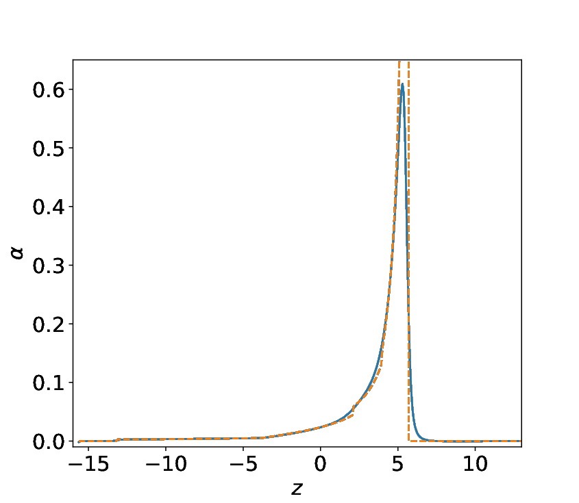
In order to verify that the analytical derivation of the perturbed density described in the previous Appendices is correct, we have carried out full hydrodynamical simulations using the ZEUS code (Stone & Norman, 1992). A good match between the analytical expressions and simulations was found. For illustration, we present here the results of the wake created by a varying-mass Plummer perturber moving at in an adiabatic simulation. In this numerical model, we have used the following parameters in code units: , , , and . Our grid model has a resolution of zones per , but we tested convergence of the results by doubling the number of grid zones per direction. Figure 15 shows along a cut at (i.e. along the -axis) at . The deviations between analytical results and numerical ones are due to the fact that the perturber in our simulations is modelled as a Plummer sphere rather than a point mass.
Appendix D Perturbed density in a more general case
It is simple to extend the derivation of for a more general form of the evolution of the mass of the perturber. Suppose that can be written as
| (71) |
where is a certain function of time to be specified. Following Appendices A and B, the wake induced by the perturber is given by , where is given in Equation (54) and
| (72) |
In particular, for a perturber that loses mass at a constat rate beyond , we have , and therefore
| (73) |