Running headline: Bayesian model selection for SECR models
Bayesian Model Selection for a Class of Spatially-Explicit Capture Recapture Models
Abstract
- 1.
A vast amount of ecological knowledge generated over the past two decades has hinged upon the ability of model selection methods to discriminate among various ecological hypotheses. The last decade has seen the rise of Bayesian hierarchical models in ecology. Consequently, commonly used tools, such as the AIC, become largely inapplicable and there appears to be no consensus about a particular model selection tool that can be universally applied.
- 2.
We focus on a specific class of competing Bayesian spatially explicit capture recapture (SECR) models and first apply some of the recommended Bayesian model selection tools: (1) Bayes Factor - using (a) Gelfand-Dey (b) harmonic mean methods, (2) Deviance Information Criterion (DIC), (3) Watanabe-Akaike’s Information Criteria (WAIC) and (4) the posterior predictive loss function. In all, we evaluate 25 variants of model selection tools in our study.
- 3.
We evaluate these model selection tools from the standpoint of model selection and parameter estimation by contrasting the choice recommended by a tool with a ‘true’ model. In all, we generate 120 simulated data sets using the true model and assess the frequency with which the true model is selected and how well the tool estimates (population size).
- 4.
We find that when information content is low in the data, no particular model selection tool can be recommended to help realise, simultaneously, both the goals of model selection and parameter estimation. In such scenarios, we recommend that practitioners utilise our application of Bayes Factor (Gelfand-Dey with MAP approximation or the harmonic mean) for parameter estimation and recommend the posterior predictive loss approach for model selection when information content is low. Generally, when we consider both the objectives together, we recommend the use of our application of Bayes Factor for Bayesian SECR models.
- 5.
Our study highlights the aspect that although new model selection tools are emerging (eg: WAIC) in the applied statistics literature, an uncritical absorption of these new tools (i.e. without assessing their efficacies for the problem at hand) into ecological practice may provide misleading inferences.
Keywords: Abundance estimation, Bayes factors, Bayesian inference, DIC, Hierarchical models, Hypothesis testing, Posterior predictive loss, WAIC.
1 Introduction
Following the highly influential text Burnham and Anderson, (2002) on model selection, ecologists and conservation biologists have drastically shifted their inferential practice from the ‘hypothesis testing’ approach to the more appropriate ‘hypothesis discrimination’ approach (Ellison,, 2004; Díaz-Francés and Soberón,, 2005). Till date, Burnham and Anderson, (2002) has been cited 43047 times (as on September 22, 2018 - Google Scholar), demonstrating the impact of this text. One may argue, that this contribution has helped increase the pace of growth in ecological knowledge because it has paved the way for researchers to draw inferences, more authentically, because of the ability to now assess the influence of various competing a priori hypotheses (models) without altering the study question to suit the restrictive hypothesis testing paradigm (Bolker,, 2008).
Since a large amount of ecological data are based on observations it permitted for ecologists to take the approach of ‘detectives’ rather than ‘hypothetico-deductive’ scientists by formulating models using likelihood functions to confront various a priori hypotheses using observational data (Hilborn and Mangel,, 1997). And by maximizing the likelihood and using a model selection tool, such as the Akaike’s Information Criterion (Burnham and Anderson,, 2002), researchers found a way to place increased faith on models favoured by such criteria. Thus, a vast amount of ecological knowledge generated, has relied on the robustness of such model selection tools in accurately discriminating hypotheses.
Recently, there has been an increased use of hierarchical models in ecology since they appear to address two important issues: (1) ecological scales are naturally hierarchical in structure and (2) hierarchical models form a natural way of incorporating the observation process (Royle and Dorazio,, 2008). And with powerful tools such as MCMC, it is now possible to confront complex ecological models with data in a Bayesian inferential framework (Bolker,, 2008). However, it remains unclear as to how to discriminate among competing hypotheses (models) because popular model selection criteria (such as AIC, BIC or DIC) (Burnham and Anderson,, 2002) aren’t easy to apply or work poorly for complex hierarchical models (Millar,, 2009).
It is well known that, asymptotically, Bayes factor is the preferred model selection tool due to its consistency property (Ghosh et al.,, 2006; Robert,, 2007; Bernardo and Smith,, 2009). However, this property holds only under certain regularity conditions that are often difficult to verify for complex models (Berger et al.,, 2003; Dass and Lee,, 2004; Ghosh and Samanta,, 2001). But more prominently, there is vast literature expressing the difficulties in computing the marginal likelihood in applied problems (Weinberg,, 2012; Chan and Eisenstat,, 2015; Wang et al.,, 2018). Hence, it becomes necessary to also consider alternatives to Bayes factor or to find novel ways of applying them in practice.
Recently, Hooten and Hobbs, (2015) summarised a wide array of Bayesian model selection methods that are available to ecologists. However, the generality of these recommendations remain unknown. Given such innate difficulties involved in discovering the ‘ideal’ model selection tool both from the standpoint of theory and its application to a broad class of models, it appears to be prudent to explore the model selection issue by conditioning, at least, on a particular class of models.
Here, we evaluate various Bayesian model selection tools on a class of Bayesian spatially explicit capture recapture (SECR) models that are now used frequently for animal density estimation (Royle et al.,, 2013). Although, previously, Goldberg et al., (2015) has attempted to apply Bayes Factor (Gelfand-Dey estimator) in an abundance estimation problem for leopards (Panthera pardus) for model selection, their approach of computing the ratio term in the estimator seems inaccurate in the context of how the denominator has to be computed according to Gelfand and Dey, (1994).
Thus, we evaluate various Bayesian model selection tools by:
- 1.
Defining a class of competing models (in our case these include the model developed in Dey et al., (2017) along with simplified alternatives) that vary both in terms of structural and model complexity.
- 2.
Simulating data sets from a ‘true’ model.
- 3.
Practically implementing a variety of Bayesian model selection tools, and in specific cases, also proposing alternatives.
- 4.
Assessing the efficacy of these implementations from the standpoint of model selection and parameter estimation.
- 5.
Providing recommendations to practitioners based on our results.
2 Methods
We describe here the true (data-generating) model which will be used for simulation of the data sets. We then fit candidate models to these data sets and apply and assess efficiencies of various model selection tools.
2.1 The candidate model set
Dey et al., (2017) develops a Bayesian SECR model for partially identified individuals as a Bayesian hierarchical model (Royle and Dorazio,, 2008). We summarise the description of the model here below.
2.1.1 Sampling situation
The notations used in this article are described in Tables 2 and 3. However, we describe a few variables and parameters for ease in the model description below.
Consider a capture-recapture survey of a species with naturally marked individuals in which two detectors are collocated at trap stations (within a bounded geographic region ) and kept active for sampling occasions. An individual can be completely identified if both the detectors record the individual simultaneously at least once during the course of study (Royle,, 2015). We assume that each detector captures some mutually exclusive attributes of an individual. These capture outcomes are recorded as binary observations and for an individual at trap station on sampling occasion corresponding to detectors 1 and 2 respectively. The paired Bernoulli outcomes give rise to bilateral spatial capture-recapture data for each individual at location on occasion . The array of a bilateral capture history for an individual is denoted by , which is of dimension . Below we provide an example of a sample data set coming out of a spatial capture-recapture survey with two detectors deployed at each station.
Example 2.1.
Suppose a capture-recapture survey is conducted where a pair of detectors (1 and 2) are deployed at each of the 3 () trap stations and kept active for 4 () sampling occasions. Two individuals get fully identified based on their obtained capture histories (captured in both cameras at least once during the survey). The capture history for each of these two fully-identified individuals is of dimension . The detection histories are tabulated in Table 1. Here, individual 1 is fully-identified owing to the capture event at trap 2 on occasion 4. Individual 1 is also fully-identified as it is captured at trap 2 on occasion 4. Due to absence of simultaneous capture events in the detection histories of the partially-identified individuals, we are uncertain about whether these histories correspond to two different individuals or to the same individual.
2.1.2 Model likelihoods
When detection rates in recorded samples are low due to failure or malfunction of detectors, capture-recapture data may comprise of individuals with uncertain identities or ‘partially identified individuals’. Dey et al., (2017) separately accounts for the process of animal arrival within detection region of a detector and detection process by conditioning on animal arrival - thus modelling the underlying mechanism by which we obtain different events leading to partial identification.
The probability of animal arrival (termed as ‘trap entry probability’) is modelled as a decreasing function of Euclidean distance between individual activity centre and trap station : . Here, is regarded as the “baseline trap entry probability” and quantifies the rate of decline in trap entry probability as increases. The observation process is parameterised in terms of detection probability which denotes the probability that any arbitrary individual is detected by a detector on some occasion given its arrival at that trap.
The obtained capture history observations and from the two detectors 1 and 2 during a spatial capture-recapture survey may not be synchronised as detectors often perform imperfectly. These two data arrays are then augmented with zero capture histories so that each of them is of dimension , being an upper bound of the population size. This also makes the dimension of the likelihood fixed in each iteration of Markov chain Monte Carlo algorithm which in turn eases computation. A vector of latent binary variables is introduced where implies that individual is a member of the population. We assume that each is a Bernoulli random variable with parameter and is independent of other ’s. Here is the proportion of individuals that are real and present within . Thus, the true population size follows the Binomial distribution with parameters and . The individuals from the two lists obtained from detector 1 and detector 2 are linked probabilistically, by introducing a latent identity variable which is a one-to-one mapping from an index set of individuals capture by detector 2 to giving the true index of each of detector 2 individuals. Without loss of generality, the true identity of each individual in the population is defined to be in the row-order of capture histories of detector 1. Then the rows of detector 2 data set are reordered as indicated by to synchronise with the individuals of the detector 1 data set . We denote this newly ordered detector 2 data set as . The joint density of is as given below:
| (2.1) |
where , is the number of times individual got detected on at least one the detectors over occasions and .
Prior to Dey et al., (2017), Royle, (2015) proposed an SECR model for partially identified individuals coming from spatial capture-recapture surveys. The joint density of under Royle, (2015) is the following:
| (2.2) |
where and denotes the probability that an individual is detected at a trap station on some occasion .
Note that, unlike model (2.1), here movement through detection region is considered inherently as a part of the observation process and is regarded as “baseline detection probability” and , although related to animal movement, is regarded as the rate of decline in detection probability. Qualitatively, the absence of in (2.2), distinguishes this model from (2.1), and can be regarded as a less general model.
Both the models, (2.1) and (2.2), can be extended by introducing a binary covariate on sex category on spatial animal movement, , as in Sollmann et al., (2011). We define as a function of the latent structural vector : , if , i.e., individual is a male; , if , i.e., individual is a female. ’s are independently and identically distributed Bernoulli random variables with parameter , being the probability that an arbitrary individual in the population is male. Let be a vector of binary observations on sex category of the captured individuals. The vector of latent missing observations in is denoted by . Assuming that covariate information on individual sex category is available, the joint density of and under Dey et al., (2017) and Royle, (2015) are, respectively, the following:
| (2.3) | ||||
| (2.4) |
where denotes the probability that an individual passes through a trap station on some occasion , denotes the probability that an individual is detected at on occasion .
The prior distributions for the model parameters , , , , , , are assumed to be independent and are provided in Table 4. To ensure that the marginal distribution of the data is well defined, we have assumed proper priors for each of these parameters (Gopalaswamy and Delampady,, 2016). We assume a uniform prior over the entire state space for each location of activity centre and that these ’s are independently distributed. is assumed to have a uniform prior distribution over the permutation space of . The prior specifications remain the same for all the model fits. The MCMC algorithm used to sample from the respective posterior density under each model is detailed in Appendix D.
Thus, we have the four models,
: Model with density (2.3),
: Model with density (2.4),
: Model with density (2.1) and
: Model with density (2.2).
Among these models, can be regarded as the most complex, general, model and can be regarded as the simplest. Therefore, in our study, we simulate data from as the true model.
2.2 Candidate model selection tools
We have considered four different Bayesian model selection methods for application and evaluation: Bayes factors, Deviance Information Criterion (DIC), Watanabe-Akaike information criterion (WAIC) and posterior predictive loss. Two popular model selection tools (AIC and BIC; Burnham and Anderson, (2002)) are not used here because because they impose restrictive assumptions on the parameter space as the sample size increases - situations often encountered in many hierarchical models (Royle and Dorazio,, 2008). For example, in the SECR models we study here, the concept of ‘number of parameters’ is unclear and we therefore cannot apply criteria such as AIC and BIC directly.
2.2.1 Bayes factors
Model comparison using Bayes factors requires the computation of the marginal likelihood, which involves the integration where denotes the model density and denotes the prior density of the parameters under . This integration is difficult to compute in practice unless the models are very simple in structure, which is often not the case in ecology. Therefore, computation of the marginal likelihood of data using MCMC methods remains to be a holy grail and is an active area of research (Wang and Meng,, 2016; Wang et al.,, 2018).
Estimation of marginal likelihood of data
Under our model settings, for models , and for the other models , . denotes the collection of all parameters and latent variables for each model as a generic notation. Specifically, let , where is the collection of scalar parameters and is the collection of all latent variables. The Gelfand-Dey estimator of marginal likelihood of data is expressed as:
| (2.5) |
where is a set of MCMC draws from the posterior and is a tuning density. It is to be noted that by specifying in (2.5), we obtain the harmonic mean estimator of the marginal likelihood
| (2.6) |
Details on these estimators and their properties can be found in Gelfand and Dey, (1994), Kass and Raftery, (1995).
For our problem at hand, the computation of (2.5) requires us to obtain the integrated likelihoods (marginals) under the different models that we consider. This becomes particularly tricky in the presence of high-dimensional latent variables such as , , , which are elements of .
We have developed two approximate approaches to compute the Gelfand-Dey estimator: the maximum a posteriori (MAP) approximation approach and the integrated likelihood (IL) approach.
Approach 1: MAP approximation
In this approach, we fix the high-dimensional variables at their MAP estimates , assuming that their posterior distributions are well summarised by these estimates which are derived from the MCMC draws. The Gelfand-Dey estimator is then computed using the formula,
| (2.7) |
where is a set of MCMC draws from the posterior . We begin with as an initial estimate of where
This estimate of posterior mode of may not be optimal since in our high dimensional parameter setting, an MCMC sample of a practical size may not be enough to extensively explore the posterior surface. We, therefore, fix one of the parameters and explore the posterior surface to find such that In this way we obtain an improved MAP estimate of , , if
Similarly, we then fix and find . This procedure is continued iteratively to eventually give us the best MAP estimate of the posterior mode (). Suitable transformations of the parameters ensure that all the points in , belong to the posterior support. The above mentioned resampling procedure is detailed in Appendix A.
Approach 2: Integrated likelihood (IL) approximation
Ideally, we would like to compute the marginal likelihood by integrating out all the latent variables with respect to their corresponding prior distributions from the model likelihoods. However, in the case of model likelihoods (2.1-2.4) this integration is not possible for the permutation vector . The integration over the variables and can be performed analytically. The integration over is evaluated numerically by partitioning the region into a sufficiently fine grid and then evaluating a Riemann sum (as direct integration can not be expressed in a closed form). This integrated likelihood can then be used in (2.5) for estimating the marginal likelihood
| (2.8) |
One downside of IL approximation approach is the lack of clarity about the interdependencies between the latent variables , , and after carrying out the integrations. The derivations of the integrated likelihoods for each of the four models are given in Appendix B by ignoring any possible interdependencies.
We have also assessed the robustness of the Gelfand-Dey estimator by computing the marginal likelihood estimates using different tuning densities, e.g., multivariate normal density, multivariate-t density with varying degrees of freedom and the truncated normal density following the suggestion of Geweke, (1999). These technical details are described in Appendix C.
2.2.2 Deviance information criterion (DIC)
Deviance is defined as . Deviance information criterion (DIC) is then defined as where is an estimate of . A model with smaller DIC value is preferred. Model comparison using DIC is not invariant to parameterisation and depends on the components of the model density to be considered as the likelihood. Spiegelhalter et al., (2002) suggests practitioners to carefully decide on the parameters of interest so that they can avoid this potential pitfall. This piece of advice is often not straightforward to implement in practice, especially when there exists inherent ambiguity in the interpretation of latent parameters. However Celeux et al., (2006) suggests several forms for DIC that can be used for different hierarchical models but does not recommend any particular form as the best.
For the computation of deviance, we have used the MAP estimate of to obtain instead of the posterior mean, due to the presence of binary latent variables and unknown permutation vectors in the likelihood. We have then computed two versions of (Hooten and Hobbs,, 2015; Gelman et al.,, 2014) using MCMC draws from as follows:
| (2.9) |
2.2.3 Watanabe-Akaike information criterion (WAIC)
The Watanabe-Akaike information criterion (WAIC) is a Bayesian version of AIC as it uses the posterior predictive distribution of the data to estimate the out-of-sample predictive accuracy of the model. Watanabe, (2010) introduced the WAIC criterion based on the assumption of independence between data points and has shown its asymptotic equivalence with cross-validation. In our model formulations, we have assumed that the different data points correspond to capture-recapture data set for each of the individuals. WAIC is then defined as A model with smaller WAIC value is preferred. In computing WAIC we partition data in terms of individuals . We compute the two commonly used versions of (Hooten and Hobbs,, 2015) using MCMC draws from as follows:
| (2.10) |
We propose another version for based on absolute error loss:
| (2.11) |
2.2.4 Posterior predictive loss
Gelfand and Ghosh, (1998) derived a model selection criterion, popularly known as the posterior predictive loss criterion, by adopting a decision theoretic approach for measuring predictive accuracy of a model. The posterior predictive loss criterion (based on a square error loss function) under our model setting is defined as follows:
| (2.12) |
where is a vector of length obtained by vectorizing observed data array and denotes replicate of the observed data. The first term in the criterion (see (2.12)) is the goodness-of-fit term while the second term can be interpreted as a penalty term for model complexity. The model with the smallest is to be preferred. In our analysis, the data set is obtained by vectorising the two binary data arrays and placing one after the other.
We compute the above expectation and variance using MCMC draws. Given an MCMC sample from , we simulate from for each . For instance, in model , denotes the collection of the parameters , , , , , , , , , . Then and .
We summarise the various model selection methods and their variants in Table 5. Considering all these model selection tools and their variants (from approximation approaches to setting tuning densities), our evaluation is carried out on 25 unique tools.
3 Evaluation of the Performance of Model Selection Methods
3.1 Simulation design and simulation scenarios
We have conducted simulations for 12 scenarios (provided in Table 6) grouped into 2 equal sized sets, to assess the performance of the models proposed here. We set = 0.3 and = 0.15 for the first set of 6 scenarios, = 0.4 and = 0.2 for the second set of 6 scenarios. We set = {(0.01, 0.3), (0.05, 0.3), (0.05, 0.5), (0.03, 0.8), (0.01, 0.9), (0.05, 0.9)}, which gives us 6 different scenarios for each of the two sets corresponding to the values taken by and . We assume that a total of 100 individuals are residing inside the state space of which 40 are male. Each of the simulation experiments is conducted within a rectangular state space of dimension 5 unit 7 unit (Figure 1), after setting a buffer of 1 unit in both horizontal and vertical directions, a trapping array of total trap stations has been set (trap spacing is 0.3 unit on axis and 0.3125 unit on axis). This meets the requirement suggested in Karanth and Nichols, (2017). Each of the traps remains active for sampling occasions simultaneously. For parameter estimation, we set the maximum possible number of individuals present in the population () at 400 for all the scenarios. The experiment is repeated times. The MCMC samples for each of the parameters are obtained (each of length 30000) and the estimates are computed using those chains with a burn-in of 10000.
Capture-recapture data sets are simulated independently under each of the 12 simulation scenarios (Table 6) under model . Recall that, model corresponds to the statistical model in (2.3) with parameter modelled in terms of individual covariate on sex category (see Section 2.1). Then each simulated data set is fitted with all the four competing model , , and .
3.2 Defining performance measures
Probability of selecting the true model
In our study, since all the data sets are simulated from model , it is considered as the true model. We have computed the proportion of times a model selection method chooses as the best. This proportion will serve as an estimate for the probability of selecting the true model. Additionally we have also computed the proportion of times a model selection method chooses , and respectively. The computed proportions of selecting these models from the simulation study will indicate the efficacy of the model selection methods.
Assessing the quality of parameter estimation.
The abundance parameter carries a lot of significance in ecology and conservation. Due to its importance, ecologists place their interests in the robustness and accuracy of its estimate, and will therefore rely on a model selection method that will achieve this. The precision and accuracy of the parameter estimates indicates the quality of the model fit and we assess this by computing the average root mean square error (average RMSE).
Suppose denotes a set of MCMC draws from the posterior distribution of an arbitrary parameter for the -th simulated data set, . Mean square error (MSE) of for -th simulated data set is estimated as Average RMSE is calculated by first averaging the estimated MSEs of different simulations and then taking the square root of the average:
The quantities related to the various Bayesian model selection methods (Section 2.2) are computed for each of the four models for the simulated data and analysis sets. First, we analyse the quality of fit of the competing models to the simulated data sets. We compute the proportion of times they favour any of these four models out of the simulations and study the consistency of these different model selection methods. These proportions are then compared with the computed average RMSEs of the parameters to study the behaviour of the model selection methods with respect to varying information content. We also generate pairwise correlation plots from the MCMC draws to study the extent of identifiability issues between various pairs of parameters as a consequence of lack of information content in the data.
4 Results of the Simulation Study
Our results suggest that the choice of the tuning density had no impact on model selection (Figures 2 and 3). Thus, we focus only on plot (a) in Figure 2 for our inferences on model selection by Bayes factor (GD-MAP approximation). Here, we observe that Bayes factor GD-MAP approximation favours in of the times under scenario 1 and favours in at least of the times under scenarios 2, 3, 4 and 7. Bayes factor is in favour of more than of the times under all the remaining scenarios 5-6 and 8-12.
The plots corresponding to the Bayes factors (GD-IL approximation) are shown in Figures 4 and 5. As seen here, GD-IL approximation performs slightly worse than the GD-MAP approximation. However, we observe that the model choices by the harmonic mean estimator of Bayes Factor performs well and favours the true model in majority of the scenarios (Figure 6).
We have considered three forms of WAIC and two forms of DIC. The corresponding plots are shown in Figure 7 (a)-(e). WAIC1, WAIC3, DIC1 and DIC2 exhibit very similar tendencies in their model choices by favouring under all the scenarios except scenario 1 and 3. These four methods favour under scenario 1. Under scenario 3, WAIC1 and DIC1 favour in majority of the times whereas WAIC3 and DIC2 favour . Like Bayes factor, these model selection methods (DICs and WAICs) also tend to favour simpler models under scenarios 1 and 3. WAIC2 largely agrees with the other WAICs (and DICs) but more often selects the true model when data sets are more informative (Figure 7 (a)-(c)). In general, DICs and WAICs seem to discourage the presence of high dimensional latent variables.
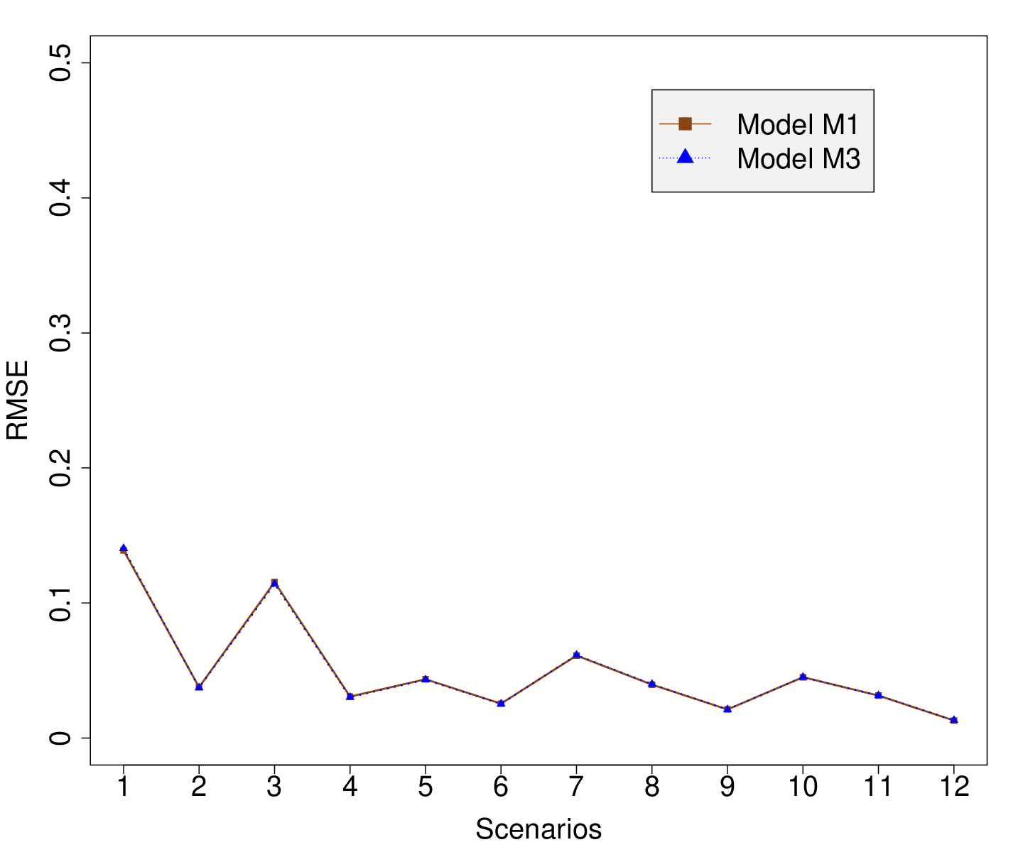
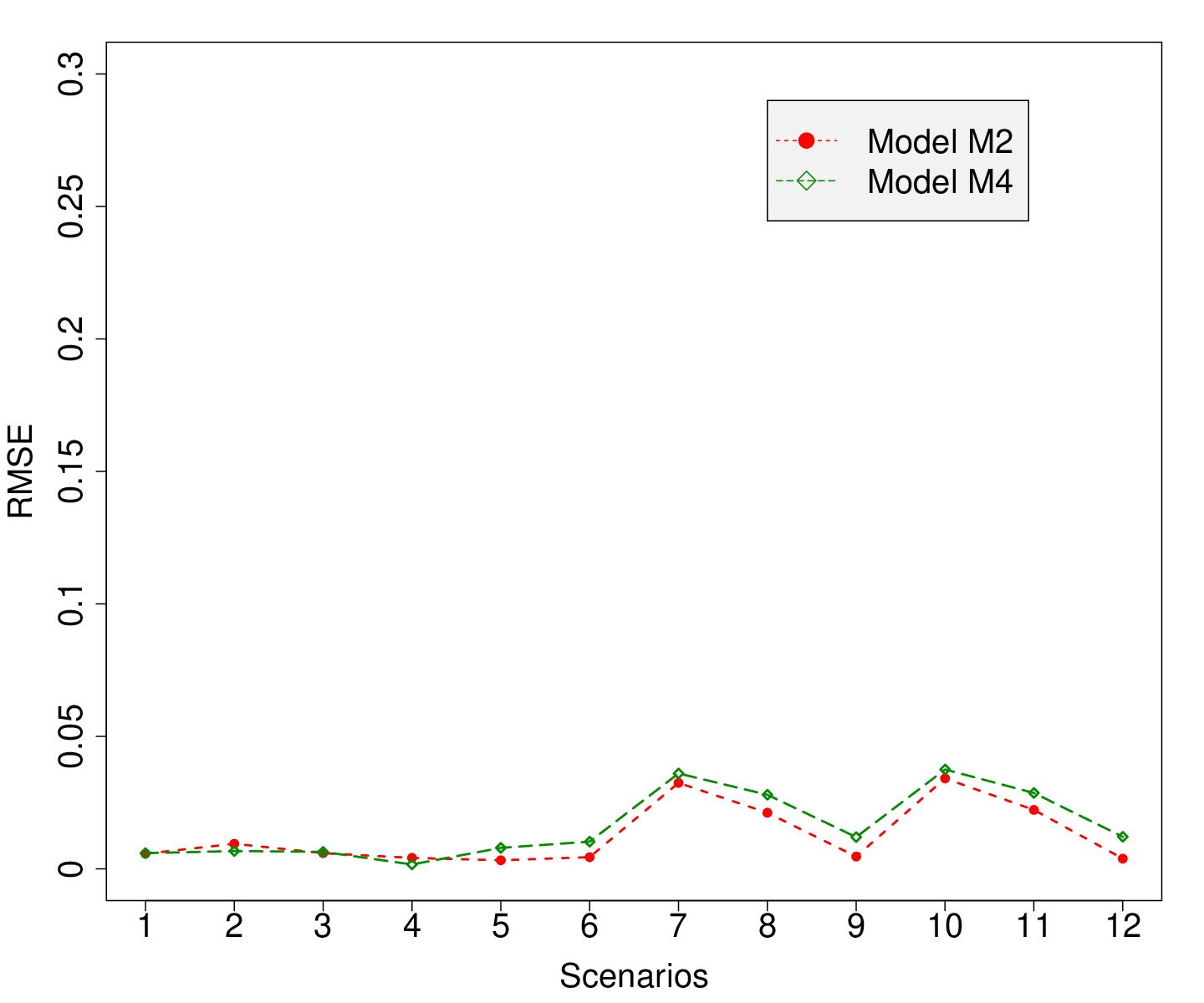
The plot showing the proportion of different model choices by posterior predictive loss is given in Figure 7(f). The posterior predictive loss criterion favours models with individual sex-covariates ( and ). Posterior predictive loss also appears to select the true model some of the times, even when there isn’t sufficient information in the data (scenarios 1 and 3). Figures 8 and 9 show the plots for the average root mean square error (average RMSE) for the parameters , , , , , , , , and . We focus our discussion based on the efficiency and accuracy in estimating . In Figure 8(a) we see that the average RMSE of is substantially higher in scenarios 1 - 3 relative to scenarios 4 - 12. Figures 10 - 15 are a representative set of scatter plots (scenarios 1, 2, 3, 7, 9, 12) meant to highlight the range of the correlation coefficient as the information content in the data sets increases. We observe that, the scatter plots of (, ) and (, ) show substantial correlation under scenarios 1 - 3 (see Figures 10 - 12). This high correlation may indicate that these parameter estimates are of poor accuracy due to inadequate sample size. However these correlations decrease for the other scenarios (e.g., 9 and 12, see Figures 14, 15), likely due to increased information content in the data.
5 Conclusions and Discussion
Contemporary practice of ecology and conservation biology relies largely on the use of model selection for hypotheses discrimination (Ellison,, 2004; Díaz-Francés and Soberón,, 2005). Simultaneously, there has been major growth in the use of hierarchical models in ecology, especially within the realm of Bayesian inference (Royle and Dorazio,, 2008; Kéry,, 2010). These models have now enabled statistical ecologists to fairly easily formulate complex ecological models and elegantly deal with the sampling process and also fit these complex models using powerful tools such as MCMC (Kéry,, 2010, e.g.,). However, the lack of availability of readymade model selection tools when practicing Bayesian inference has sometimes motivated ecologists to continue using likelihood-based inferences, merely because one can use well known model selection tools such as the AIC (Burnham and Anderson,, 2002) for inference.
To provide a context for this argument, in the spatial capture-recapture literature, we have essentially seen the development of three important likelihood functions: (1) Borchers and Efford, (2008), (2) Royle et al., (2009) and (3) Royle et al., (2015). Inferences, for the models (1) and (3) are by maximizing the likelihood, while the inference for (2) is Bayesian. We note with interest, that one of the reasons for the development of (3), was motivated on the pretext that model selection is much easier (using known tools such as the AIC) for practitioners using the likelihood approach, in spite of the problem having been already solved in the Bayesian context (Royle et al.,, 2013). It is specially of concern in the context of the models we study here in that investigators may be forced to integrate out ’s (activity centres of individuals) in order to construct tractable likelihoods and thus oversimplifying ecological reality.
In this study, we have tried to implement some selected Bayesian model selection methods on a specific class of advanced Bayesian SECR models (Royle,, 2015 - with and without sex covariates; Dey et al.,, 2017 - with and without sex covariates) dealing with partially identified individuals. We have found our Bayes factor implementation using the Gelfand-Dey estimator (using the MAP approximation approach) to be the preferred choice as a model selection method over a wide range of simulation scenarios. This approach appears to work particularly well when information content in the data is moderate to high. The IL approximation approach also worked well, but not as well as the MAP approximation approach perhaps because, there exists interdependency between some of the latent variables.
However, implementing Bayes factors for model selection using the Gelfand-Dey estimator (with MAP approximation) can be computationally intensive and complicated while setting up. Interestingly, our study demonstrates that obtaining Bayes factors using harmonic mean approach for marginal likelihood computation is less demanding but yet serves as a very good model selection method. This finding deviates from the popular view among applied scientists that it is futile to estimate the marginal likelihood using the harmomic mean approach (Lartillot and Philippe,, 2006; Xie et al.,, 2011). We surmise that this finding may be attributed to the fact that when we bind the priors (as we have done, but for other reasons) and not permit extremely low probabilities to occur at the tails, many of the criticisms (Lartillot and Philippe,, 2006; Xie et al.,, 2011) may become irrelevant in practice, but this would require further enquiry.
As our simulation study shows, the two goals of model selection and parameter estimation cannot be simultaneously achieved under certain circumstances (scenarios 1 - 3), especially when information content is low (indicated by high RMSE values and correlation coefficients). Hence, researchers have to clearly prioritize their objectives prior to data analysis. If the goal, for example, is to find a model that best estimates population size , then we recommend the use of Bayes factor (Gelfand-Dey with MAP approximation) or the Bayes factor (harmonic mean, due to its simplicity) because these appear to provide the most reliable estimates of over all the simulation scenarios. However, if researchers are only interested to select the true model, especially when data are less informative (scenarios 1 - 3), we recommend the posterior predictive loss approach since they favour the true model nearly a 1/3rd of the times in situations with such low information content. Of course, the dual objectives of model selection and parameter estimation are met when information content is moderate or high (scenarios 4 - 12) and as stated previously, we recommend either Bayes factor (Gelfand-Dey with MAP approximation) or Bayes factor (harmonic mean) in such cases. However, the posterior predictive loss (with the squared error loss function) as used here, does not select the true model when information content is moderate to high.
We also do not recommend the use of DICs or WAICs, since they do not appear to outcompete other model selection tools (either from the standpoint of model selection or parameter estimation) in any of the simulation scenarios. This is an interesting finding, because tools such as WAIC are much newer tools developed by applied Bayesians to provide answers to a wide range of contemporary model selection problems involving hierarchical models (Hooten and Hobbs,, 2015; Gelman et al.,, 2014). Thus, our study brings back focus on the need to assess the strength of inference from a model selection method by conditioning on a true model and consequently evaluating a competing set of model selection methods prior to selecting the most appropriate one for the problem on hand.
Our approach does not, strictly speaking, permit us to draw conclusions and make inferences on the most suitable model selection tools beyond the restrictive set of competing models and the settings we have used in this study. However, at the risk of making a claim beyond our case study, we would recommend the use of the Bayes Factor (Gelfand-Dey with MAP approximation or the harmonic mean estimator) for most Bayesian SECR models and perhaps to much larger class of hierarchical models in ecology (Royle et al.,, 2013). We note with interest that it is also unclear whether the routinely used AIC works as an appropriate model selection tool for MLE-based SECR models as discussed in Efford and Mowat, (2014).
6 Acknowledgements
We thank the Indian Statistical Institute for financial and administrative support. AMG thanks the Wildlife Conservation Society, New York for partial funding support.
7 Authors contribution
SD, MD and AMG conceived the ideas and designed methodology; SD, MD and AMG analysed the simulated data; SD, MD and AMG did the writing of the manuscript. All authors contributed critically to the drafts and gave final approval for publication.
| Detector 1 | Detector 2 | |||||||||
| Occasion | 1 | 2 | 3 | 4 | Occasion | 1 | 2 | 3 | 4 | |
| Trap | Trap | |||||||||
| Fully-identified individual 1 | 1 | 0 | 1 | 0 | 1 | 1 | 0 | 0 | 1 | 0 |
| 2 | 1 | 0 | 0 | \raisebox{-0.9pt} {1}⃝ | 2 | 0 | 0 | 0 | \raisebox{-0.9pt} {1}⃝ | |
| 3 | 0 | 0 | 1 | 1 | 3 | 1 | 0 | 0 | 0 | |
| Fully-identified individual 2 | 1 | \raisebox{-0.9pt} {1}⃝ | 0 | 0 | 0 | 1 | \raisebox{-0.9pt} {1}⃝ | 1 | 0 | 0 |
| 2 | 0 | 0 | 0 | 1 | 2 | 0 | 0 | 0 | 0 | |
| 3 | 1 | 1 | 0 | 0 | 3 | 0 | 0 | 1 | 0 | |
| Partially-identified individual | 1 | 1 | 0 | 0 | 1 | 1 | - | - | - | - |
| 2 | 0 | 0 | 1 | 0 | 2 | - | - | - | - | |
| 3 | 0 | 0 | 0 | 0 | 3 | - | - | - | - | |
| Partially-identified individual | 1 | - | - | - | - | 1 | 0 | 0 | 1 | 0 |
| 2 | - | - | - | - | 2 | 1 | 0 | 0 | 0 | |
| 3 | - | - | - | - | 3 | 0 | 0 | 1 | 0 | |
| Variables and parameters | Definition |
|---|---|
| A bounded geographic region of scientific or operational relevance | |
| where a population of individuals of certain species reside. | |
| Population size of the superpopulation, i.e., the number of | |
| individuals within . | |
| Maximum number of individuals within the state space . | |
| This is a fixed quantity defined by the investigator. | |
| Proportion of individuals that are real and present within . | |
| Probability that an individual is male. | |
| Number of trap stations in . | |
| Number of sampling occasions. | |
| Maximum permissible value of movement range for each | |
| individual during the survey. | |
| Baseline trap entry probability in the models and , | |
| i.e., probability that an individual passes through a trap station | |
| assuming its centre of activity is also located at that trap station. | |
| Baseline detection probability in the models and , | |
| i.e., probability that an individual is detected by a detector | |
| assuming its centre of activity is also located at that trap station. | |
| measures the spatial extent of movement around individual | |
| activity centre. for male individuals, for | |
| female individuals. | |
| Euclidean distance between points and . | |
| Probability that an individual passes through a trap station | |
| on some occasion and is modelled as a function | |
| of individual covariate on sex category . | |
| Probability that an individual passes through a trap station | |
| on some occasion . | |
| Probability that an individual is detected by a detector on | |
| some occasion given that it is present at that trap. | |
| Notations pertaining to | Definition |
| model selection tools | |
| Gelfand-Dey estimator of the marginal likelihood of data . | |
| Harmonic mean estimator of the marginal likelihood of data . | |
| Correction term for bias due to overfitting in DIC criterion. | |
| Correction term for bias due to overfitting in WAIC criterion. | |
| Posterior predictive loss criterion. |
| Latent variables | Definition |
|---|---|
| Locations of the activity centres of animals within . | |
| Location of individual ’s activity centre. | |
| A vector of Bernoulli variables, if individual is present. | |
| A vector of Bernoulli variables, if individual is male | |
| in the population and if it is a female. | |
| Vector of “missing” binary observations on sexes of the | |
| list of individuals. | |
| A one to one mapping from index set of individuals captured | |
| by detector 2 to providing the true index of each | |
| detector 2 individuals. | |
| Data | Definition |
| Location of trap station for detectors. | |
| Vector of “recorded” binary observations on sexes of the | |
| captured individuals. | |
| if individual is detected in detector 1 at trap station | |
| on occasion , if not detected in detector 1. | |
| Number of times individual got detected | |
| in detector 1 over trap stations and occasions. | |
| if individual is detected in detector 2 at trap station | |
| on occasion , if not detected in detector 2. | |
| Number of times individual got detected | |
| in detector 2 over trap stations and occasions. | |
| Number of fully identified individuals, each of them is captured | |
| by both the detectors on at least one occasion. | |
| Array of individual specific capture histories obtained by | |
| detector 1 (dimension ). | |
| Array of individual specific capture histories obtained by | |
| detector 2 (dimension ). | |
| Zero augmented array of individual specific capture histories | |
| corresponding to detector 1 (dimension ). | |
| Zero augmented array of individual specific capture histories | |
| corresponding to detector 2 (dimension ). | |
| Reordered according to (dimension ). | |
| Number of times individual got detected at trap | |
| on at least one of its sides over occasions. | |
| Number of times individual got detected on at least | |
| one of its sides over traps and occasions. |
| Parameters | Prior | Parameters | Prior |
|---|---|---|---|
| Uniform | Uniform | ||
| Uniform | Uniform | ||
| Uniform | Uniform | ||
| Uniform | Uniform |
| Sl. no. | Model selection | Variant | Approximation | Choices of | Eq. No. |
| method | method | tuning density | |||
| 1. | Bayes factor | Gelfand-Dey | MAP | Multivariate normal density, multivar- | (2.7) |
| estimator | iate- density with degrees of freedom | ||||
| 10, 100, 500, 1000, 10000 and truncated | |||||
| multivariate normal density with confid- | |||||
| ence coefficients 0.90, 0,95, 0.99. | |||||
| 2 | Bayes factor | Gelfand-Dey | IL | -Do- | (2.8) |
| estimator | |||||
| 3. | Bayes factor | Harmonic mean | - | - | (2.6) |
| estimator | |||||
| 4. | DIC | MAP | - | (2.9) | |
| 5. | DIC | MAP | - | (2.9) | |
| 6. | WAIC | - | - | (2.10) | |
| 7. | WAIC | - | - | (2.10) | |
| 8. | WAIC | - | - | (2.11) | |
| 9. | Posterior | - | - | - | (2.12) |
| predictive loss |
| Scenario | |||||||
|---|---|---|---|---|---|---|---|
| 1 | 400 | 100 | 40 | 0.01 | 0.3 | 0.3 | 0.15 |
| 2 | 400 | 100 | 40 | 0.01 | 0.9 | 0.3 | 0.15 |
| 3 | 400 | 100 | 40 | 0.01 | 0.3 | 0.4 | 0.20 |
| 4 | 400 | 100 | 40 | 0.01 | 0.9 | 0.4 | 0.20 |
| 5 | 400 | 100 | 40 | 0.03 | 0.8 | 0.3 | 0.15 |
| 6 | 400 | 100 | 40 | 0.03 | 0.8 | 0.4 | 0.20 |
| 7 | 400 | 100 | 40 | 0.05 | 0.3 | 0.3 | 0.15 |
| 8 | 400 | 100 | 40 | 0.05 | 0.5 | 0.3 | 0.15 |
| 9 | 400 | 100 | 40 | 0.05 | 0.9 | 0.3 | 0.15 |
| 10 | 400 | 100 | 40 | 0.05 | 0.3 | 0.4 | 0.20 |
| 11 | 400 | 100 | 40 | 0.05 | 0.5 | 0.4 | 0.20 |
| 12 | 400 | 100 | 40 | 0.05 | 0.9 | 0.4 | 0.20 |

| (a) | (b) |
 |
 |
| (c) | (d) |
 |
|
| (e) | (f) |
|
|
| (a) | (b) |
|---|---|
 |
 |
| (c) | |
 |
| (a) | (b) |
 |
|
| (c) | (d) |
|
|
| (e) | (f) |
|
|
| (a) | (b) |
|---|---|
 |
|
| (c) | |
|

| (a) | (b) |
 |
 |
| (c) | (d) |
 |
 |
| (e) | (f) |
 |
 |
 |
 |
 |
 |
 |
 |
 |
 |
 |
 |


References
- Berger et al., (2003) Berger, J. O., Ghosh, J. K., and Mukhopadhyay, N. (2003). Approximations and consistency of Bayes factors as model dimension grows. Journal of Statistical Planning and Inference, 112(1):241–258.
- Bernardo and Smith, (2009) Bernardo, J. M. and Smith, A. F. (2009). Bayesian theory, volume 405. John Wiley & Sons.
- Bolker, (2008) Bolker, B. M. (2008). Ecological models and data in R. Princeton University Press.
- Borchers and Efford, (2008) Borchers, D. L. and Efford, M. G. (2008). Spatially Explicit Maximum Likelihood Methods for Capture–Recapture Studies. Biometrics, 64(2):377–385.
- Burnham and Anderson, (2002) Burnham, K. P. and Anderson, D. R. (2002). Model Selection and Multimodel Inference: A Practical Information–Theoretic Approach. Springer-Verlag, New York, Second edition.
- Celeux et al., (2006) Celeux, G., Forbes, F., Robert, C. P., and Titterington, D. M. (2006). Deviance information criteria for missing data models. Bayesian analysis, 1(4):651–673.
- Chan and Eisenstat, (2015) Chan, J. C. C. and Eisenstat, E. (2015). Marginal likelihood estimation with the Cross-Entropy method. Econometric Reviews, 34(3):256–285.
- Dass and Lee, (2004) Dass, S. C. and Lee, J. (2004). A note on the consistency of Bayes factors for testing point null versus non-parametric alternatives. Journal of Statistical Planning and Inference, 119(1):143–152.
- Dey et al., (2017) Dey, S., Delampady, M., Karanth, K. U., and Gopalaswamy, A. M. (2017). A spatially explicit capture recapture model for partially identified individuals when trap detection rate is less than one. ArXiv e-prints arXiv:1712.10035.
- Díaz-Francés and Soberón, (2005) Díaz-Francés, E. and Soberón, J. (2005). Statistical estimation and model selection of species-accumulation functions. Conservation Biology, 19(2):569–573.
- Efford and Mowat, (2014) Efford, M. G. and Mowat, G. (2014). Compensatory heterogeneity in spatially explicit capture-recapture data. Ecology, 95(5):1341–1348.
- Ellison, (2004) Ellison, A. M. (2004). Bayesian inference in ecology. Ecology Letters, 7(6):509–520.
- Gelfand and Dey, (1994) Gelfand, A. E. and Dey, D. K. (1994). Bayesian model choice: asymptotics and exact calculations. Journal of the Royal Statistical Society. Series B (Methodological), pages 501–514.
- Gelfand and Ghosh, (1998) Gelfand, A. E. and Ghosh, S. K. (1998). Model choice: a minimum posterior predictive loss approach. Biometrika, pages 1–11.
- Gelman et al., (2014) Gelman, A., Carlin, J. B., Stern, H. S., Dunson, D. B., Vehtari, A., and Rubin, D. B. (2014). Bayesian data analysis. CRC press, Taylor & Francis Group, Boca Raton, FL, Third edition.
- Geweke, (1999) Geweke, J. (1999). Using simulation methods for Bayesian econometric models: inference, development, and communication. Econometric reviews, 18(1):1–73.
- Ghosh et al., (2006) Ghosh, J. K., Delampady, M., and Samanta, T. (2006). An Introduction to Bayesian Analysis, Theory and Methods. Springer Texts in Statistics. Springer, New York.
- Ghosh and Samanta, (2001) Ghosh, J. K. and Samanta, T. (2001). Model selection–An overview. Current Science, 80(9):1135–1144.
- Goldberg et al., (2015) Goldberg, J. F., Tempa, T., Norbu, N., Hebblewhite, M., Mills, L. S., Wangchuk, T. R., and Lukacs, P. (2015). Examining temporal sample scale and model choice with spatial capture-recapture models in the common leopard Panthera pardus. PloS one, 10(11):e0140757.
- Gopalaswamy and Delampady, (2016) Gopalaswamy, A. M. and Delampady, M. (2016). Examining posterior propriety in the Bayesian analysis of capture–recapture models. arXiv preprint arXiv:1611.02403.
- Hilborn and Mangel, (1997) Hilborn, R. and Mangel, M. (1997). The ecological detective: confronting models with data, volume 28. Princeton University Press.
- Hooten and Hobbs, (2015) Hooten, M. B. and Hobbs, N. T. (2015). A guide to Bayesian model selection for ecologists. Ecological Monographs, 85(1):3–28.
- Karanth and Nichols, (2017) Karanth, K. U. and Nichols, J. D. (2017). Methods For Monitoring Tiger And Prey Populations. Springer.
- Kass and Raftery, (1995) Kass, R. E. and Raftery, A. E. (1995). Bayes factors. Journal of the american statistical association, 90(430):773–795.
- Kéry, (2010) Kéry, M. (2010). Introduction to WinBUGS for ecologists: Bayesian approach to regression, ANOVA, mixed models and related analyses. Academic Press.
- Lartillot and Philippe, (2006) Lartillot, N. and Philippe, H. (2006). Computing Bayes factors using thermodynamic integration. Systematic biology, 55(2):195–207.
- Millar, (2009) Millar, R. B. (2009). Comparison of hierarchical Bayesian models for overdispersed count data using DIC and Bayes’ factors. Biometrics, 65(3):962–969.
- Robert, (2007) Robert, C. P. (2007). The Bayesian Choice, From Decision–Theoretic Foundations to Computational Implementation. Springer Texts in Statistics. Springer, New York, Second edition.
- Royle, (2015) Royle, J. A. (2015). Spatial capture-recapture with partial identity. arXiv preprint arXiv:1503.06873.
- Royle et al., (2013) Royle, J. A., Chandler, R. B., Sollmann, R., and Gardner, B. (2013). Spatial Capture–Recapture. Academic Press.
- Royle and Dorazio, (2008) Royle, J. A. and Dorazio, R. M. (2008). Hierarchical modeling and inference in ecology: the analysis of data from populations, metapopulations and communities. Academic Press.
- Royle et al., (2009) Royle, J. A., Karanth, K. U., Gopalaswamy, A. M., and Kumar, N. S. (2009). Bayesian inference in camera trapping studies for a class of spatial capture-recapture models. Ecology, 90(11):3233–3244.
- Royle et al., (2015) Royle, J. A., Sutherland, C., Fuller, A. K., and Sun, C. C. (2015). Likelihood analysis of spatial capture–recapture models for stratified or class structured populations. Ecosphere, 6(2):1–11.
- Sollmann et al., (2011) Sollmann, R., Furtado, M. M., Gardner, B., Hofer, H., Jácomo, A. T. A., Tôrres, N. M., and Silveira, L. (2011). Improving density estimates for elusive carnivores: accounting for sex-specific detection and movements using spatial capture–recapture models for jaguars in central brazil. Biological Conservation, 144(3):1017–1024.
- Spiegelhalter et al., (2002) Spiegelhalter, D. J., Best, N. G., Carlin, B. P., and van der Linde, A. (2002). Bayesian measures of model complexity and fit. Journal of the Royal Statistical Society. Series B. Statistical Methodology, 64(4):583–639.
- Wang and Meng, (2016) Wang, L. and Meng, X.-L. (2016). Warp bridge sampling: the next generation. arXiv preprint arXiv:1609.07690.
- Wang et al., (2018) Wang, Y.-B., Chen, M.-H., Kuo, L., and Lewis, P. O. (2018). A new Monte Carlo method for estimating marginal likelihoods. Bayesian analysis, 13(2):311.
- Watanabe, (2010) Watanabe, S. (2010). Asymptotic equivalence of Bayes cross validation and widely applicable information criterion in singular learning theory. Journal of Machine Learning Research, 11(Dec):3571–3594.
- Weinberg, (2012) Weinberg, M. D. (2012). Computing the Bayes factor from a Markov chain Monte Carlo simulation of the posterior distribution. Bayesian Analysis, 7(3):737–770.
- Xie et al., (2011) Xie, W., Lewis, P. O., Fan, Y., Kuo, L., and Chen, M.-H. (2011). Improving marginal likelihood estimation for Bayesian phylogenetic model selection. Systematic Biology, 60(2):150–160.