Efficient Representation of Topologically Ordered States with Restricted Boltzmann Machines
Abstract
Representation by neural networks, in particular by restricted Boltzmann machines (RBM), has provided a powerful computational tool to solve quantum many-body problems. An important open question is how to characterize which class of quantum states can be efficiently represented with RBMs. Here, we show that RBMs can efficiently represent a wide class of many-body entangled states with rich exotic topological orders. This includes: (1) ground states of double semion and twisted quantum double models with intrinsic topological orders; (2) states of the AKLT model and two-dimensional CZX model with symmetry protected topological orders; (3) states of Haah code model with fracton topological order; (4) (generalized) stabilizer states and hypergraph states that are important for quantum information protocols. One twisted quantum double model state considered here harbors non-abelian anyon excitations. Our result shows that it is possible to study a variety of quantum models with exotic topological orders and rich physics using the RBM computational toolbox.
Introduction.—Deep learning has become a powerful tool with wide applications (LeCun et al. 2015; Goodfellow et al. 2016). Recently, deep learning methods have attracted considerable attention in quantum physics (Biamonte et al. 2017; Ciliberto et al. 2018), especially for attacking quantum many-body problems. The difficulty of quantum many-body problems mainly originates from the exponential growth of the Hilbert space dimension. To overcome this exponential difficulty, researchers traditionally use tensor network methods (Schollwöck 2011; Verstraete et al. 2008; Schuch et al. 2008) and Quantum Monte Carlo (QMC) simulation (Ceperley and Alder 1986). However, QMC methods suffer from the sign problem (Loh et al. 1990); Tensor network methods have difficulty to deal with high dimensional systems (Schuch et al. 2007) or systems with massive entanglement (Verstraete et al. 2006). These issues call for mew method.
Being one of the fundamental building block of deep learning, the neural network has been recently employed as a compact representation of quantum many-body states (Carleo and Troyer 2017; Deng et al. 2017a; Clark 2018; Gao and Duan 2017; Huang and Moore 2017; Deng et al. 2017b; Cai and Liu 2018; Chen et al. 2018; Glasser et al. 2018; Jia et al. 2018; Carleo et al. 2018). Many variants of neural networks have been investigated numerically or theoretically, such as the restricted Boltzmann machines (RBM) (Carleo and Troyer 2017; Deng et al. 2017a; Gao and Duan 2017; Jia et al. 2018), the deep Boltzmann machine (DBM) (Gao and Duan 2017; Carleo et al. 2018; Huang and Moore 2017), and the feed-forward Neural Network (FNN)(Cai and Liu 2018). The RBM ansatz have also been investigated for quantum information protocols (Torlai et al. 2018; Jónsson et al. 2018; Deng 2018). We focus here on the RBM states which work efficiently during variational optimization although the representational power of which is somewhat limited. An important open issue is how to characterize the class of quantum many-body states that can be represented by the RBMs.
In the past decades, the studies of topological order (Zeng et al. 2015; Wen 2004), which are beyond the framework of Landau’s symmetry breaking paradigm (Landau and Lifshitz 1980), have attracted tremendous attention. There are several types of topological ordered states: the intrinsic topological ordered states feature unliftable ground state degeneracy through local perturbations; the symmetry protected topological (SPT) ordered states with a given symmetry cannot be smoothly deformed into each other without a phase transition if the deformation preserves the symmetry; the fracton topological ordered states harbor point excitations that are immobile in the three-dimensional space, i.e., fractons. While several studies have shown that the RBM can capture simple many-body states such as graph/cluster states (Gao and Duan 2017; Deng et al. 2017a) and toric/surface code states (Gao and Duan 2017; Deng et al. 2017a; Jia et al. 2018), no single study exists which represents other more exotic topological states in the condensed matter physics (Wen 2004; Zeng et al. 2015; Chen et al. 2012; Chiu et al. 2016).
In this paper, we use tools from quantum information to construct the RBM representations for other notable many-body states, focusing on different topologically ordered states. Many of exotic condensed matter topological states can be described by powerful quantum information tools: (i) the hypergraph state formalism which generalizes the graph-state formalism; (ii) the stabilizer formalism (Gottesman 1997) which describes most of the quantum error correction code; (iii) the XS-stabilizer formalism (Ni et al. 2015) which generalizes stabilizer formalism. These formalisms themselves are vital for quantum error correction (Gottesman 1997), classical simulation of quantum circuits (Gottesman 1998) and Bell’s nonlocality (Gachechiladze et al. 2016; Guhne et al. 2014; Bell 1964; Brunner et al. 2014; Gühne et al. 2005). We prove these states of (i-iii) can be represented by the RBM efficiently based on the properties of their wave functions. We also propose a unary representation to generalize RBM state to higher spin systems.
These tools from quantum information provide recipes for constructing RBM representation within their formalism. The stabilizer formalism describes many fracton models (Haah 2011; Yoshida 2013; Ma et al. 2017; Vijay et al. 2015; Vijay et al. 2016; Chamon 2005) such as Haah’s code (Haah 2011). Concerning the intrinsic topological order, we show tbe RBM states can capture double semion of string-net model (Levin and Wen 2005; Gu et al. 2009) and many twisted quantum double model (Kitaev 2003; Hu et al. 2013; Beigi et al. 2011) using their XS-stabilizer description. For symmetry protected topological orders, we give exact constructions of the AKLT model (Affleck et al. 1987; Affleck et al. 1988) with the unary representation. We also consider RBM representation for other SPT models such as the two-dimensional (2D) CZX model (Chen et al. 2011). Our exact representation results provide insights and a powerful tool for future studies of quantum topological phase transitions and quantum information protocols.
RBM state.— We first recall the definition of RBM state and describe notations. In the computational basis, a quantum wave function of -qubit can be expressed as with , where the is a complex function of binary variables . We use valued vertices instead of valued vertices for convenience. In the case of RBM, , where the weight is a complex quadratic function of binary variables. While a Boltzmann machine allows arbitrary intra-layer connection, in RBM the visible neurons only connect to hidden neurons . Let the number of visible neurons be and the number of hidden neurons be . We say the representation is efficient if . The whole wave function writes
| (1) |
with effective angles .
We depict this paper’s roadmap in Fig. 1. RBM states (Hein et al. 2006) have been shown to represent graph states efficiently (Gao and Duan 2017; Deng et al. 2017a) (recall the wave function of graph states takes the form (up to a normalization factor), where denotes an edge linking the -th and -th qubits represented by visible neurons , ). There are various ways to generalize graph states. Hypergraph states (Rossi et al. 2013) generalize graph states by introducing more than two body correlation factors such as . Stabilizer states generalize graph states through additional local Clifford operations (Dehaene and De Moor 2003; Van den Nest et al. 2004; Grassl et al. 2002), which impose parity constraints and extra phases. XS-stabilizer states (Ni et al. 2015) combines 3-body correlation factors from hypergraph state and parity constraints from stabilizer states. A parity constraint: can be realized by a hidden neuron that connects to each of these visible neurons with weight function (aff). Next we derive the RBM representation of multi-body correlation factors (hypergraph states) and the unary representation, making all the states in Fig. 1 can be represented by the RBM.
The unary RBM representation.— To study higher spin systems, we propose the unary representation. The idea of unary representation is best illustrated using an example, as depicted in Fig. 2. We use three neurons (qubits) to represent a spin-1: , and by restricting these three neurons (qubits) to the subspace spanned by and . This can be done by using two hidden neurons (blue neurons in Fig. 2) (S). Our unary representation is simpler than multi-value neurons or encoded binary neurons in distinguishing and decoding basis states. We will use this unary representation to represent the AKLT state.
RBM representation of hypergraph states.— Hypergraphs generalize graphs by allowing an edge can join any number of vertices. We define an edge that connects vertices a -hyperedge. Given a mathematical hypergraph, the wave function of its corresponding hypergraph state (Rossi et al. 2013) takes the form:. The notation means that these vertices are connected by a -hyperedge. We illustrate the correspondence in Fig. 3. We now extend RBM representation to hypergraph states.
Theorem 1
Restricted Boltzmann machines can represent any hypergraph states efficiently and exactly.
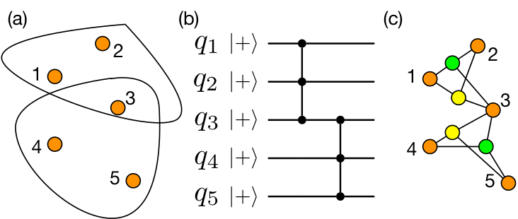
In the main text, we take the graph with 3-hyperedges as an example; it will be useful later for representation of XS-stabilizer states and SPT states. Precisely, we make use of the following decomposition:
| (2) |
where , and . Thus, the exact RBM representation of uses two hidden neurons, as shown in Fig. 3 (c). The method for decomposing can be extended to treat for arbitrary with hidden neurons (S).
RBM representation of XS/Pauli-stabilizer states.— The Pauli stabilizer formalism generalizes graph states by applying some local Clifford transformations (Van den Nest et al. 2004; Schlingemann 2002). The XS-stabilizer formalism generalizes the Pauli stabilizer formalism (Ni et al. 2015) by changing the single qubit Pauli group to Pauli- group where and . We have the following theorem based on the key observation that the wave function of the stabilizer state first proved in (Aggarwal and Calderbank 2008; Dehaene and De Moor 2003) and the similar result on XS-stabilizer state proved in (Ni et al. 2015).
Theorem 2
Restricted Boltzmann machines can represent any Pauli-stabilizer states and XS-stabilizer states efficiently and exactly.
Let satisfies and . The wave functions of every Pauli-stabilizer state and XS-stabilizer state on qubits can be written as the closed form of
| (3) | ||||
| (4) |
where , and are linear, quadratic and cubic polynomials of with integer coefficients respectively. The are affine (linear terms plus constant term) functions of some subsets of . Moreover, these polynomials , and along with can be determined efficiently from the given stabilizers.
Given this wave function, we can easily deduce its RBM representation: First, the parts correspond to parity constraints, which RBM can represent. Meanwhile, functions that are products of , , , and can also be represented by RBM using techniques used for graph states and hypergraph states. In the case of stabilizer states, we provide a new proof of the closed form wave function as follow: First, a stabilizer state can be generated from a Clifford circuit (Gottesman 1997) consisting of , and gates. From the encoding circuit, the stabilizer state can be represented by a DBM in the closed form Eq. (3) directly. Then we can iteratively reduce it to an RBM while still keep the closed form (S).
We can make use of local Clifford equivalence between stabilizer state and graph states (Van den Nest et al. 2004; Hostens et al. 2005a) to further simplify our procedure. We can choose the encoding circuit based on fact that every stabilizer state can be chosen to be locally equivalent to a graph state such that only at most a single or gate acting on each qubit (Hostens et al. 2005a). Then, the number of hidden neurons used to represent hidden variables is fewer than the number of acting on each qubit. In total, the number of hidden neurons needed is of order . The is number of edges in the corresponding graph, and is at most ; however we do not usually encounter graph states from dense graphs (Anders and Briegel 2006), typically only or even hidden neurons are needed. Our representation method is effective and optimal. Next, we describe topological states with different topological orders within our quantum information framework. These topological states can be represented as RBM efficiently.
Fracton topological order.— The Pauli stabilizer formalism covers most of the fracton topological order models (Haah 2011; Yoshida 2013; Ma et al. 2017; Chamon 2005), such as Haah’s code (Haah 2011). Stabilizers of Haah’s code involve two types of stabilizers on eight spins: eight s and eight s in each cube.
Intrinsic topological order.— We now consider RBM representation for some notable XS stabilizer states: the double semion (an example of string-net model (Levin and Wen 2005)) and many twist quantum double models. We define the double semion model on a honeycomb lattice with one qubit per edge. The wave function of double semion is: . In the XS-stabilizer formalism, this model has two types of stabilizer operators (Ni et al. 2015): corresponding to the vertex and the face respectively.
Quantum double models (Kitaev 2003) are generalizations of the toric code that describe systems of abelian and non-abelian anyons. Twisted quantum double models further generalizes quantum double models (Kitaev 2006; Buerschaper 2014; Kitaev 2003; Kitaev 2006; Hu et al. 2013; Beigi et al. 2011) and are Hamiltonian realizations of Dijkgraaf-Witten topological Chern-Simons theories (Dijkgraaf and Witten 1990). Many twisted quantum double models fit into the XS-stabilizer formalism (Ni et al. 2015), thus can be represented as RBM exactly. Examples include twisted quantum double model with the group and different twists on a triangular lattice, where is the third cohomology group. The case includes the double semion. It is known (Ni et al. 2015; de Wild Propitius 1997) that a non-trivial twist from harbors non-abelian anyon excitations.
Symmetry protected topological order.— The AKLT model (Affleck et al. 1988; Affleck et al. 1987) is a one-dimensional spin-1 model with symmetric protected topological order. When imposing the periodic boundary condition, the unique ground state , in terms of the matrix product state, writes
| (5) |
where , and . Alternatively, matrix product states can be described as projected entangled pairs states (PEPS) (Zeng et al. 2015). As shown in Fig. 4, every red line is a EPR pair . Each shaded circle represents a projection from two spins of dimension 2 to a physical degree of dimension (spin-1). where the summation is over and . After using unary representation, in the quantum circuit language, the projection is a map that maps and . We find such a quantum circuit made of Clifford gate, as shown in Fig. 4(b). Because all operations are Clifford gates, the whole quantum state is a Pauli stabilizer state restricted to the single excitation subspace. Thus it can be represented by RBM with unary hidden neurons (blue neurons in Fig. 2) and other hidden neurons (S).
We also show RBM can represent other symmetry-protected topologically ordered states. These examples include the 2D CZX model (with symmetry), and Yoshida’s CCZ model (Yoshida 2016) (with symmetry). The ground state of the 2D CZX model (Chen et al. 2011) is a tensor product of GHZ states on each plaquette. Because GHZ state belongs to stabilizer states, RBM can exactly represent the ground state of the 2D CZX model. Similar to SPT cluster states, the ground state of Yoshida’s CCZ model (Yoshida 2013) on the trivalent lattice is a hypergraph state with 3-hyperedges. Thus it can also be represented efficiently by RBMs.
Discussions.— This paper sets out to investigate different topological models with RBM representation using tools from quantum information such as the (XS) stabilizer and the (hyper) graph-state formalisms. The most significant findings are the fact that RBM states can capture ground states of exotic models with different types of topological orders, including intrinsic topological orders, symmetry protected topological orders and fracton topological orders. It remains open whether RBM can capture additional string-net models with more exotic non-abelian anyon excitations such as the states of the double Fibonacci model (Levin and Wen 2005). RBM state may be helpful in investigating symmetry enriched topological order (Cheng et al. 2017) and symmetry fractionalization (Chen 2017). Our exact representation results provide useful guidance for future numerical studies on topological phase transitions.
Our results are also of interest from the quantum information perspective. The Gottesman-Knill theorem (Gottesman 1998; Anders and Briegel 2006; Aaronson and Gottesman 2004) states that stabilizer dynamics can be efficiently simulated. Our result which shows RBM states contain stabilizer states suggests classical simulation of an unknown larger family of quantum circuits may benefit from the RBM representation (Jónsson et al. 2018). Because hypergraph states allow for an exponentially increasing violation of the Bell inequalities (Gachechiladze et al. 2016; Guhne et al. 2014; Bell 1964; Brunner et al. 2014), our results provide analytical evidence for numerical studies (Deng et al. 2017a) on estimating maximum violation of Bell inequalities.
Acknowledgements.
We thank Giuseppe Carleo, Dong-Ling Deng, Sheng-Tao Wang, Mingji Xia, Shunyu Yao, Fan Ye, Zhengyu Zhang and You Zhou for helpful discussions. This work was supported by Tsinghua University and the National Key Research and Development Program of China (2016YFA0301902). Note added.— After completion of this work, a preprint appeared in arXiv (Zhang et al. 2018) which gives a different method to represent stabilizer states with the restricted Boltzmann machine.References
- LeCun et al. (2015) Yann LeCun, Yoshua Bengio, and Geoffrey Hinton, “Deep learning,” Nature 521, 436–444 (2015).
- Goodfellow et al. (2016) Ian Goodfellow, Yoshua Bengio, Aaron Courville, and Yoshua Bengio, Deep learning, Vol. 1 (MIT press Cambridge, 2016).
- Biamonte et al. (2017) Jacob Biamonte, Peter Wittek, Nicola Pancotti, Patrick Rebentrost, Nathan Wiebe, and Seth Lloyd, “Quantum machine learning,” Nature 549, 195–202 (2017).
- Ciliberto et al. (2018) Carlo Ciliberto, Mark Herbster, Alessandro Davide Ialongo, Massimiliano Pontil, Andrea Rocchetto, Simone Severini, and Leonard Wossnig, “Quantum machine learning: a classical perspective,” Proc. R. Soc. A 474, 20170551 (2018).
- Schollwöck (2011) Ulrich Schollwöck, “The density-matrix renormalization group in the age of matrix product states,” Annals of Physics 326, 96–192 (2011).
- Verstraete et al. (2008) Frank Verstraete, Valentin Murg, and J Ignacio Cirac, “Matrix product states, projected entangled pair states, and variational renormalization group methods for quantum spin systems,” Advances in Physics 57, 143–224 (2008).
- Schuch et al. (2008) Norbert Schuch, Michael M. Wolf, Frank Verstraete, and J. Ignacio Cirac, “Simulation of quantum many-body systems with strings of operators and monte carlo tensor contractions,” Phys. Rev. Lett. 100, 040501 (2008).
- Ceperley and Alder (1986) David Ceperley and Berni Alder, “Quantum monte carlo,” Science 231, 555–560 (1986).
- Loh et al. (1990) E. Y. Loh, J. E. Gubernatis, R. T. Scalettar, S. R. White, D. J. Scalapino, and R. L. Sugar, “Sign problem in the numerical simulation of many-electron systems,” Phys. Rev. B 41, 9301–9307 (1990).
- Schuch et al. (2007) Norbert Schuch, Michael M. Wolf, Frank Verstraete, and J. Ignacio Cirac, “Computational complexity of projected entangled pair states,” Phys. Rev. Lett. 98, 140506 (2007).
- Verstraete et al. (2006) F. Verstraete, M. M. Wolf, D. Perez-Garcia, and J. I. Cirac, “Criticality, the area law, and the computational power of projected entangled pair states,” Phys. Rev. Lett. 96, 220601 (2006).
- Carleo and Troyer (2017) Giuseppe Carleo and Matthias Troyer, “Solving the quantum many-body problem with artificial neural networks,” Science 355, 602–606 (2017), http://science.sciencemag.org/content/355/6325/602.full.pdf .
- Deng et al. (2017a) Dong-Ling Deng, Xiaopeng Li, and S. Das Sarma, “Machine learning topological states,” Phys. Rev. B 96, 195145 (2017a).
- Clark (2018) Stephen R Clark, “Unifying neural-network quantum states and correlator product states via tensor networks,” Journal of Physics A: Mathematical and Theoretical 51, 135301 (2018).
- Gao and Duan (2017) Xun Gao and Lu-Ming Duan, “Efficient representation of quantum many-body states with deep neural networks,” Nature Communications 8, 662 (2017).
- Huang and Moore (2017) Yichen Huang and Joel E Moore, “Neural network representation of tensor network and chiral states,” arXiv preprint arXiv:1701.06246 (2017).
- Deng et al. (2017b) Dong-Ling Deng, Xiaopeng Li, and S. Das Sarma, “Quantum entanglement in neural network states,” Phys. Rev. X 7, 021021 (2017b).
- Cai and Liu (2018) Zi Cai and Jinguo Liu, “Approximating quantum many-body wave functions using artificial neural networks,” Phys. Rev. B 97, 035116 (2018).
- Chen et al. (2018) Jing Chen, Song Cheng, Haidong Xie, Lei Wang, and Tao Xiang, “Equivalence of restricted boltzmann machines and tensor network states,” Phys. Rev. B 97, 085104 (2018).
- Glasser et al. (2018) Ivan Glasser, Nicola Pancotti, Moritz August, Ivan D. Rodriguez, and J. Ignacio Cirac, “Neural-network quantum states, string-bond states, and chiral topological states,” Phys. Rev. X 8, 011006 (2018).
- Jia et al. (2018) Zhih-Ahn Jia, Yuan-Hang Zhang, Yu-Chun Wu, Guang-Can Guo, and Guo-Ping Guo, “Efficient machine learning representations of surface code with boundaries, defects, domain walls and twists,” arXiv preprint arXiv:1802.03738 (2018).
- Carleo et al. (2018) Giuseppe Carleo, Yusuke Nomura, and Masatoshi Imada, “Constructing exact representations of quantum many-body systems with deep neural networks,” arXiv preprint arXiv:1802.09558 (2018).
- Torlai et al. (2018) Giacomo Torlai, Guglielmo Mazzola, Juan Carrasquilla, Matthias Troyer, Roger Melko, and Giuseppe Carleo, “Neural-network quantum state tomography,” Nature Physics 14, 447–450 (2018).
- Jónsson et al. (2018) Bjarni Jónsson, Bela Bauer, and Giuseppe Carleo, “Neural-network states for the classical simulation of quantum computing,” arXiv preprint arXiv:1808.05232 (2018).
- Deng (2018) Dong-Ling Deng, “Machine learning detection of bell nonlocality in quantum many-body systems,” Phys. Rev. Lett. 120, 240402 (2018).
- Zeng et al. (2015) Bei Zeng, Xie Chen, Duan-Lu Zhou, and Xiao-Gang Wen, “Quantum information meets quantum matter–from quantum entanglement to topological phase in many-body systems,” arXiv preprint arXiv:1508.02595 (2015).
- Wen (2004) Xiao-Gang Wen, Quantum field theory of many-body systems: from the origin of sound to an origin of light and electrons (Oxford University Press on Demand, 2004).
- Landau and Lifshitz (1980) LD Landau and EM Lifshitz, “Statistical physics, vol. 5,” Course of theoretical physics 30 (1980).
- Chen et al. (2012) Xie Chen, Zheng-Cheng Gu, Zheng-Xin Liu, and Xiao-Gang Wen, “Symmetry-protected topological orders in interacting bosonic systems,” Science 338, 1604–1606 (2012), http://science.sciencemag.org/content/338/6114/1604.full.pdf .
- Chiu et al. (2016) Ching-Kai Chiu, Jeffrey C. Y. Teo, Andreas P. Schnyder, and Shinsei Ryu, “Classification of topological quantum matter with symmetries,” Rev. Mod. Phys. 88, 035005 (2016).
- Gottesman (1997) Daniel Gottesman, “Stabilizer codes and quantum error correction,” arXiv preprint quant-ph/9705052 (1997).
- Ni et al. (2015) Xiaotong Ni, Oliver Buerschaper, and Maarten Van den Nest, “A non-commuting stabilizer formalism,” Journal of Mathematical Physics 56, 052201 (2015).
- Gottesman (1998) Daniel Gottesman, “The heisenberg representation of quantum computers,” arXiv preprint quant-ph/9807006 (1998).
- Gachechiladze et al. (2016) Mariami Gachechiladze, Costantino Budroni, and Otfried Guhne, “Extreme violation of local realism in quantum hypergraph states,” Phys. Rev. Lett. 116, 070401 (2016).
- Guhne et al. (2014) Otfried Guhne, Marti Cuquet, Frank ES Steinhoff, Tobias Moroder, Matteo Rossi, Dagmar Bruß, Barbara Kraus, and Chiara Macchiavello, “Entanglement and nonclassical properties of hypergraph states,” Journal of Physics A: Mathematical and Theoretical 47, 335303 (2014).
- Bell (1964) J. S. Bell, “On the einstein podolsky rosen paradox,” Physics Physique Fizika 1, 195–200 (1964).
- Brunner et al. (2014) Nicolas Brunner, Daniel Cavalcanti, Stefano Pironio, Valerio Scarani, and Stephanie Wehner, “Bell nonlocality,” Rev. Mod. Phys. 86, 419–478 (2014).
- Gühne et al. (2005) Otfried Gühne, Géza Tóth, Philipp Hyllus, and Hans J. Briegel, “Bell inequalities for graph states,” Phys. Rev. Lett. 95, 120405 (2005).
- Haah (2011) Jeongwan Haah, “Local stabilizer codes in three dimensions without string logical operators,” Phys. Rev. A 83, 042330 (2011).
- Yoshida (2013) Beni Yoshida, “Exotic topological order in fractal spin liquids,” Phys. Rev. B 88, 125122 (2013).
- Ma et al. (2017) Han Ma, Ethan Lake, Xie Chen, and Michael Hermele, “Fracton topological order via coupled layers,” Phys. Rev. B 95, 245126 (2017).
- Vijay et al. (2015) Sagar Vijay, Jeongwan Haah, and Liang Fu, “A new kind of topological quantum order: A dimensional hierarchy of quasiparticles built from stationary excitations,” Phys. Rev. B 92, 235136 (2015).
- Vijay et al. (2016) Sagar Vijay, Jeongwan Haah, and Liang Fu, “Fracton topological order, generalized lattice gauge theory, and duality,” Phys. Rev. B 94, 235157 (2016).
- Chamon (2005) Claudio Chamon, “Quantum glassiness in strongly correlated clean systems: An example of topological overprotection,” Phys. Rev. Lett. 94, 040402 (2005).
- Levin and Wen (2005) Michael A. Levin and Xiao-Gang Wen, “String-net condensation: A physical mechanism for topological phases,” Phys. Rev. B 71, 045110 (2005).
- Gu et al. (2009) Zheng-Cheng Gu, Michael Levin, Brian Swingle, and Xiao-Gang Wen, “Tensor-product representations for string-net condensed states,” Phys. Rev. B 79, 085118 (2009).
- Kitaev (2003) A.Yu. Kitaev, “Fault-tolerant quantum computation by anyons,” Annals of Physics 303, 2 – 30 (2003).
- Hu et al. (2013) Yuting Hu, Yidun Wan, and Yong-Shi Wu, “Twisted quantum double model of topological phases in two dimensions,” Phys. Rev. B 87, 125114 (2013).
- Beigi et al. (2011) Salman Beigi, Peter W Shor, and Daniel Whalen, “The quantum double model with boundary: condensations and symmetries,” Communications in mathematical physics 306, 663–694 (2011).
- Affleck et al. (1987) Ian Affleck, Tom Kennedy, Elliott H. Lieb, and Hal Tasaki, “Rigorous results on valence-bond ground states in antiferromagnets,” Phys. Rev. Lett. 59, 799–802 (1987).
- Affleck et al. (1988) Ian Affleck, Tom Kennedy, Elliott H Lieb, and Hal Tasaki, “Valence bond ground states in isotropic quantum antiferromagnets,” in Condensed matter physics and exactly soluble models (Springer, 1988) pp. 253–304.
- Chen et al. (2011) Xie Chen, Zheng-Xin Liu, and Xiao-Gang Wen, “Two-dimensional symmetry-protected topological orders and their protected gapless edge excitations,” Phys. Rev. B 84, 235141 (2011).
- Hein et al. (2006) Marc Hein, Wolfgang Dür, Jens Eisert, Robert Raussendorf, M Nest, and H-J Briegel, “Entanglement in graph states and its applications,” arXiv preprint quant-ph/0602096 (2006).
- Rossi et al. (2013) Matteo Rossi, M Huber, D Bruß, and C Macchiavello, “Quantum hypergraph states,” New Journal of Physics 15, 113022 (2013).
- Dehaene and De Moor (2003) Jeroen Dehaene and Bart De Moor, “Clifford group, stabilizer states, and linear and quadratic operations over gf(2),” Phys. Rev. A 68, 042318 (2003).
- Van den Nest et al. (2004) Maarten Van den Nest, Jeroen Dehaene, and Bart De Moor, “Graphical description of the action of local Clifford transformations on graph states,” Phys. Rev. A 69, 022316 (2004).
- Grassl et al. (2002) Markus Grassl, Andreas Klappenecker, and Martin Rotteler, “Graphs, quadratic forms, and quantum codes,” in Information Theory, 2002. Proceedings. 2002 IEEE International Symposium on (IEEE, 2002) p. 45.
- (58) This can be generalized to affine function: both equals to 0 and 1 are allowed. The RBM representation of toric code uses the case of .
- (59) See Supplementary Material for more details.
- Schlingemann (2002) D Schlingemann, “Stabilizer Codes Can Be Realized As Graph Codes,” Quantum Info. Comput. 2, 307–323 (2002).
- Aggarwal and Calderbank (2008) Vaneet Aggarwal and A Robert Calderbank, “Boolean functions, projection operators, and quantum error correcting codes,” IEEE Transactions on Information Theory 54, 1700–1707 (2008).
- Hostens et al. (2005a) Erik Hostens, Jeroen Dehaene, and Bart De Moor, “Stabilizer states and clifford operations for systems of arbitrary dimensions and modular arithmetic,” Phys. Rev. A 71, 042315 (2005a).
- Anders and Briegel (2006) Simon Anders and Hans J Briegel, “Fast simulation of stabilizer circuits using a graph-state representation,” Phys. Rev. A 73, 022334 (2006).
- Kitaev (2006) Alexei Kitaev, “Anyons in an exactly solved model and beyond,” Annals of Physics 321, 2–111 (2006).
- Buerschaper (2014) Oliver Buerschaper, “Twisted injectivity in projected entangled pair states and the classification of quantum phases,” Annals of Physics 351, 447–476 (2014).
- Dijkgraaf and Witten (1990) Robbert Dijkgraaf and Edward Witten, “Topological gauge theories and group cohomology,” Communications in Mathematical Physics 129, 393–429 (1990).
- de Wild Propitius (1997) Mark de Wild Propitius, “(spontaneously broken) abelian chern-simons theories,” Nuclear Physics B 489, 297–359 (1997).
- Yoshida (2016) Beni Yoshida, “Topological phases with generalized global symmetries,” Phys. Rev. B 93, 155131 (2016).
- Cheng et al. (2017) Meng Cheng, Zheng-Cheng Gu, Shenghan Jiang, and Yang Qi, “Exactly solvable models for symmetry-enriched topological phases,” Phys. Rev. B 96, 115107 (2017).
- Chen (2017) Xie Chen, “Symmetry fractionalization in two dimensional topological phases,” Reviews in Physics 2, 3–18 (2017).
- Aaronson and Gottesman (2004) Scott Aaronson and Daniel Gottesman, “Improved simulation of stabilizer circuits,” Phys. Rev. A 70, 052328 (2004).
- Zhang et al. (2018) Yuan-Hang Zhang, Zhih-Ahn Jia, Yu-Chun Wu, and Guang-Can Guo, “An efficient algorithmic way to construct boltzmann machine representations for arbitrary stabilizer code,” arXiv preprint arXiv:1809.08631 (2018).
- Cai et al. (2014) Jin-Yi Cai, Pinyan Lu, and Mingji Xia, “The complexity of complex weighted boolean# csp,” Journal of Computer and System Sciences 80, 217–236 (2014).
- Cai et al. (2018) Jin-Yi Cai, Heng Guo, and Tyson Williams, “Clifford gates in the holant framework,” Theoretical Computer Science (2018).
- Hostens et al. (2005b) Erik Hostens, Jeroen Dehaene, and Bart De Moor, “Stabilizer states and clifford operations for systems of arbitrary dimensions and modular arithmetic,” Phys. Rev. A 71, 042315 (2005b).
Appendix A Detailed derivation of RBM representations of hypergraph states
First we recall the definition of quantum hypergraph state in more detail. Mathematically, hypergraphs are generalization of graphs in which an edge may connect more than two vertices. Formally, a hypergraph is a pair where is a set of element called vertices, and is a subset of , where is the power set of . Given a mathematical hypergraph, the corresponding quantum state can be generated by following similar steps in constructing a graph state: first, assign to each vertex a qubit and initialize each qubit as ; Then, whenever there is hyperedge, perform a controlled- operation between all connected qubits; if the qubits are connected by a -hyperedge, then perform . As a result, the hypergraph state and its wave function (Rossi et al. 2013) take the form
| (6) | ||||
Next, we give a detailed derivation of realizing correlation factor of the type using restricted Boltzmann machines. We first recall which relates to graph states from (Gao and Duan 2017):
| (7) | ||||
Note the above equation Eq. 7 is only true for . By , we have an explicitly formula fo :
Then we consider with the following decomposition.
Let . The above equation simplifies to
The RBM can represent first part by definition. We consider the second part as a RBM with two hidden neurons and set equations:
Solving the above equation, we get , , and
Solve the above system of equations, we obtain
In fact, this construction can be extended to any function of the form . The proof goes as follows. First, we generlize our construction a bit to simulate the correlation factor by two hidden neurons. Setting the equation:
Simplifying above equation, we obtain
Solving the system of equation, we get
Now we proceed to construct RBM representation for . Note equals to 1 only if , i.e., .For convenience, we first consider
The trick of the construction is to introduce the function
Then the function can be chosen as (the idea is similar to Lagrange polynomial method)
Then by substitution we get
In principle we can factorize into the form of , which can then be simulated by RBM term by term.
Now we remark on the relation between our decomposition and Eq. (22) in (Carleo et al. 2018). These two mainly differs from in the choose of the basis. We use basis in contrast to the basis in (Carleo et al. 2018). This difference leads to several consequences. First, in the basis, only equals to when all the equals to 1. While in the basis, equals to or if number of -1 in is even/odd. That’s the reason why latter decomposition only needs two hidden neurons. If we derive a similar RBM expression of our n-body gadget from Eq. (22) in (Carleo et al. 2018) directly, hidden neurons is needed. In contrast our cost is . Meanwhile, the correlation factor of graph/hypergraph states is somewhat meaningless in the basis.
Appendix B Derivation details of RBM unary representations
Restricting three neurons only take values from 100, 010 and 001 is equvalently to construct to RBM representation of state: . This can be done by two hidden neurons as follow. Consider the function
We find a decomposition of :
which can be simulated using two hidden neurons using the method from the last section. The weight can be computed.
The notion of state has been generalized for qubits to Dicke state. We define state to be a uniform superposition of all computational basis states where is a Hamming weight bit string. It can be done by using nearly the same technique from the last section.
Appendix C Derivation details on RBM representation of stabilizer states
The wave function can be represented by a DBM as follow. We denote visible neurons as and hidden neurons as . For convenience. We unify the notation of these neurons as here. As shown in Fig. 5: each gate corresponds to two neurons with the weight ; each gates corresponds to one neuron with the weight (even though each single qubit matrix has two indices); each gate corresponds to two neurons with the weight . Multiplying together and sum over all the hidden indices, we can get the wave function of the stabilizer state:
| (8) |
where and are affine (with linear and constant terms) and quadratic (without linear term) polynomials with integer coefficients.
Next, we reduce this DBM to a RBM with the following strategy: after eliminating a for some , the remaining term still keeps the form shown in Eq. 8 except an additional parity constraint on some of . Here, we consider the effect of eliminating in detail:
- (1)
If the coefficient of in is 0 or 2, ignoring the terms not depending on , the remaining in Eq. 8 could be written as:
where means constraint and is an affine polynomial involves those which interact with in and constant terms which are the coefficients of in . There are two cases for :
(1.1) If only involves visible neurons, we can put this constraint before the summation in Eq. 8;
(1.2) If involves hidden neurons, e.g. , then we can solve the equation by . After the summation of , the only remaining terms are those satisfying so we can replace by in and by in (because ) in Eq. 8. The key point is: the coefficients of quadratic terms in are always 2 thus they keeps the same form as the terms in the summation of Eq. 8 after summation over and .
- (2)
After eliminating all the hidden variables, the wave function could be written as the form of Eq. (3) . The parity constraints could be represented by a hidden neuron with the corresponding visible neurons as shown before.
Our method also generalizes conveniently to qudit stabilizer states (Hostens et al. 2005b) with the proposed unary representation.