Effect of intra-channel baseline migration on
the measured visibility and spatial power spectrum

The analog power spectral density (intensity as a continuous function of frequency) from a source pixel can be represented as accurately as needed by specifying it at discrete micro-tones, whose spacing, $\epsilon$ can be made as small as needed. The pixel’s double-sided power spectral density and auto-correlation, real and even functions in frequency and delay respectively are:

The interferometer measures the received radiation electric field as a function of aperture position and time,

$E(x,t)$ is sampled at a period of $T_{s}=(2f_{end})^{-1}$. To analyse baseline migration which happens at the original radio frequency, we use direct RF (rather than the usual down-converted intermediate frequency (IF)) sampling. If analysing for a system with IF down-conversion, the signal band needs to be mapped (one-to-one) back to the original RF band while the spectral resolution is what is achieved in the IF band. Let $N_{\epsilon}$ be the number of samples contained in one microtone period ($T_{\epsilon}=\epsilon^{-1}$). It is also the number of microtones contained in the band $|f|\leq f_{end}$.

In FX mode, the detected field is first transformed into spectral channels/bins using DFT and then spatially correlated over the aperture. The observation time for each DFT cycle is $T={f_{res}}^{-1}=({\sigma\epsilon})^{-1}=\sigma^{-1}T_{\epsilon}=N_{tot}T_{s}$. The $b^{th}$ spectral bin corresponds to a bin-center frequency of $f_{b}=bf_{res}$, for $|b|\leq(K+B_{max})$. The DFT spectrum at the position $x$ is:

The real-valued window function $h(t)$ to control spectral leakage between channels, is non-zero for $0\leq t\leq T$. It is zero-padded till $|t|=0.5T_{\epsilon}=0.5\sigma T$ and replicated (aliased) thereafter so that its complex spectral response $H(m)$ is discretised to the microtone resolution for $|m|\leq 0.5(N_{\epsilon}-1)$. The adjacent microtones won’t be orthogonal since the cycle time T is smaller than the microtone period $T_{\epsilon}$ by a factor $\sigma^{-1}$. This causes spectral leakage from microtones adjacent to $f_{b}$.

Treating equation () as if it were an $N_{\epsilon}$ point DFT spectrum at the microtone resolution, centered at the microtone $b\sigma$ and substituting equation (2.1) in it, the spectral samples at the DFT resolution $f_{res}$ appear as a discrete convolution between the microtone field spectral samples and the window’s spectral response interpolated to the microtone resolution:

Let $b+$ and $b-$ indicate positive and negative valued bin indices. The DFT process ensures conjugate symmetry with respect to $b$ since the sign of the microtones follows that of $b$:

Consider the case where there is no inter-channel migration i.e., having access to visibility at the same baseline $u_{0}$ for all bin-center frequencies ($f_{b}$) either from an errorless gridding interpolation or from dense enough packing of antenna elements. In such a scenario, the chromaticity of baselines is from within the spectral channel.

The visibility at a baseline $u_{0}$ for the $b^{th}$ bin is measured by correlating (over x with a shift of $u_{0}\lambda_{b}=u_{0}C/(|b|f_{res})$) the radiation field’s DFT spectrum for that bin and then time-averaging this over several DFT cycles.

Let $L(x)$ be the aperture illumination or weighting function and its spatial auto-correlation, the spatial transfer function, be $W_{u_{0}}$. For a point-source at $l=l_{0}$,

$E^{src}_{m}$, the field emitted by the source at a microtone frequency $m\epsilon$, is a random phase process whose mean amplitude-squared gives the source’s power spectral density (per unit microtone spacing) at this microtone frequency namely $P_{m}$ (equation 1). Since it is considered to be of zero-mean and statistically independent for distinct microtones, $\left\langle E^{src}_{m_{1}}.(E^{src}_{m_{2}})^{*}\right\rangle_{t}=P_{m_{1}}\delta_{m_{1},m_{2}}$.

The term $mu_{0}/(|b|\sigma)$ can be interpreted as the modified baseline due to intra-channel migration at the micro-tone level. At the channel center frequency $f_{b}$ to which the measured visibility is referenced, let $x_{b}$ be the antenna separation that would provide the baseline $u_{0}=x_{b}/\lambda_{b}=x_{b}|b|\sigma\epsilon/C$. The same antenna separation provides a modified baseline $u_{m}$ at any other microtone frequency ($m\epsilon$):

Then we can compare the measured visibility from the modified baseline, $V_{u_{m}}(b)$ against the visibility for the ideal case, $V_{u_{0}}(b)$ where the baseline would have been maintained at $u_{0}$ at the microtone level.

$P_{u_{m}}(m)$ and $P_{u_{0}}(m)$ can be interpreted as the power spectral response at a channel centered around $m$, with and without intra-channel migration respectively. $H(m)$ can be taken to have a significant spectral response only till a few (say, $B_{sig}$) channel widths i.e., $H(m)=0$ for $|m|\geq B_{sig}\sigma$. For reasons like aliasing, the useful signal band $f_{band}=(f_{min},\>f_{max}]$ is made a subset of the system band $f_{sys}=(f_{start},\>f_{end}]$. If $f_{band}$ can be confined to bins with $|b|>(K+B_{sig})$ and $|b|\leq((K+B_{max}-B_{sig})\;=(K+B_{max-sig}))$, then (using $\star$ for discrete convolution),

In the (u, f)-plane where the visibility measurements are made (Morales M. F. et al. 2012), this can be interpreted as in figure 1. In the ideal case, the same phase of the visibility gets sampled for all microtones that go into a channel. In the measured case, there is a shift in the phase of the visibility sampled at one microtone compared to its neighbour and this shift increases as the ratio of the channel center frequency to the spectral resolution (i.e., channel index) decreases. In other words, the extent (baseline span) of intra-channel migration increases as this ratio decreases.

$R_{h}(\tau)$, the inverse transform of $|H(m)|^{2}$, is the auto-correlation of $h(t)$ normalised to microtone period. We’ll use $R^{T}_{h}(\tau)$ to denote the inverse transform of $\sigma|H(m)|^{2}$ which normalises it to the duration of the window’s existence, $T$.

Using $R_{src}(\tau)$ (equation 2) for the source’s auto-correlation, the fourier transforms of $P_{u_{m}}(m)$ and $P_{u_{0}}(m)$ can be seen as instrumental windowing on the source’s auto-correlation:

When there is intra-channel migration, the auto-correlation peaks of the source and the window function are not aligned anymore. This attenuates the measured visibility. The mis-alignment $(l_{0}u_{0}T)/(|b|)$ is frequency dependent and keeps increasing as $b$, the ratio of channel center frequency to the resolution decreases in magnitude.

Here $P_{m}=P_{l_{0}}$ is constant and $R_{src}(\tau)=P_{l_{0}}\delta(\tau)$ (equations 1 and 2). Let $Q_{l_{0}}\;=\;\sigma P_{l_{0}}$ be the power spectral density from the pixel $l_{0}$ per unit channel spacing. Let the normalization to $h(t)$ be such that, $R^{T}_{h}(0)$, its power content within $0\leq t\leq T$ is unity. This makes

Due to equation (), the manner in which the measured visibility decays spectrally at a channel $b$ depends on how $R^{T}_{h}(\tau)$ decorrelates at a lag of $(|l_{0}u_{0}|T/|b|)$. Since the latter exists only for $|\tau|<T$ and $(nT_{\epsilon}-T)<|\tau|<(nT_{\epsilon}+T)$, where $n=1,2,...\infty$ denotes the aliasing index, the former exists only if the channel index, $|b|=(|f_{b}|/f_{res})$ lies within a certain range $(R^{0}\cup R^{n})$.

The region $R^{0}$ is $(|l_{0}u_{0}|,\;\infty)$ and $R^{n}$ is

Let $\Delta R^{0}$ and $\Delta R^{n}$ denote the range of bins provided by the corresponding regions over which the visibility does not vanish. Given that $\sigma>>1$,

The per-baseline worst-case (maximum) for $|l_{0}u_{0}|$ is

Those ranges of $R^{n}$ that fall below $(K+B_{sig})$ do not count. Moreover $\Delta R^{n}$ is less than one and the frequency range provided by $R^{n}$ over all n does not exceed $f_{res}$ so long as $(\pi^{2}/3).(M_{u_{max}}/\sigma^{2})<1$ and so at most one spectral channel can have $|b|$ within $R^{n}$. We ignore this and consider only $R^{0}$ as the valid range for $|b|$.

$R^{0}$ can be rewritten as $((K+B_{crit})<|b|\leq(K+B_{max-sig}))$ where,

For this to hold in the entire field-of-view, $-l_{max}\leq l_{0}\leq l_{max}$, we need:

We’ll proceed by posing the visibility attenuation as a function of the channel center frequency.

The sub-unity factor $G$ is maximum for the highest frequency and falls gradually to a minimum at $|b|=(K+B_{crit})$. This minimum is zero if $B_{crit}>B_{sig}$ where the former equals ($|l_{0}u_{0}|-K$). Figure 2 shows the magnitude of visibility as a function of frequency.

For the natural DFT window, $h(t)=1\;for\;0\leq t\leq T$,

The average slope of decay across the band is,

If $(|b|-K)<B_{max-sig}\ll K$ i.e., $f_{band}\ll f_{start}$, we have this linearization, $G_{u_{0}}(b)\approx G^{base}+G^{sloping}(b)$ such that for $B_{crit}<(|b|-K)\leq B_{max-sig}$,

For $B_{crit}\ngtr B_{sig}$, the amplitude of the sloping term relative to the base term is,

As the spectral resolution worsens, $\sigma$ increases while $K$ decreases and the slope of G increases. When $(K+B_{sig})=f_{min}/f_{res}$ drops below $|l_{0}u_{0}|$, $B_{crit}(u_{0})$ exceeds $B_{sig}$ and $V_{u_{m}}$ starts to shrink from its original span of $f_{band}$ and in the delay domain this stretches the delay spectrum as shown in section 3. This crossing first happens at the highest baseline and thereafter the extent of shrinking $(B_{crit}(u_{0})-B_{sig})$ increases with baseline.

A polyphase filter bank (PFB) (Chennamangalam J. 2016; Price D. C. 2018; Thompson, A. R., Moran, J. M., Swenson, Jr., G. W. 2017) can be seen as a window that operates over several cycles (say, $P$) of buffered data, thereby shrinking the inter-channel spectral leakage by P (i.e., $H(m)$ becomes $H(mP)$ and the channel resolution improves from $f_{res}$ to $f_{res}/P$). Now there are $P$ times more channels to cover the same signal band and we decimate the DFT output taking every $P^{th}$ channel so that the spacing between adjacent channels is still kept at $f_{res}$. Then equations (2.1) and () become,

where the first $((P-1)T/T_{s})$ time samples come from buffered data of the previous $(P-1)$ DFT cycles and the last $T/T_{s}$ samples are the fresh data input for the current cycle. $P$ is the order (number of taps) of polyphase FIR filters used in the filter bank. Since the PFB window function is $P$ times larger compared to a window operating on an isolated cycle of DFT input (also referred to as a single block fourier transform (SBFT)), $R^{T}_{h}(\tau)$ remains non-zero for $|\tau|<PT$ as opposed to $T$. This relaxes the region $R^{0}$ to $(|l_{0}u_{0}|/P,\;\infty)$.

Although spectral leakage from microtones outside the channel has been reduced relative to SBFT, the microtones from the same channel cause the measured visibility to decay and possibly vanish if $M_{u_{max}}/(K+B_{sig})=M_{u_{max}}.f_{res}/f_{min}$ exceeds $P$.

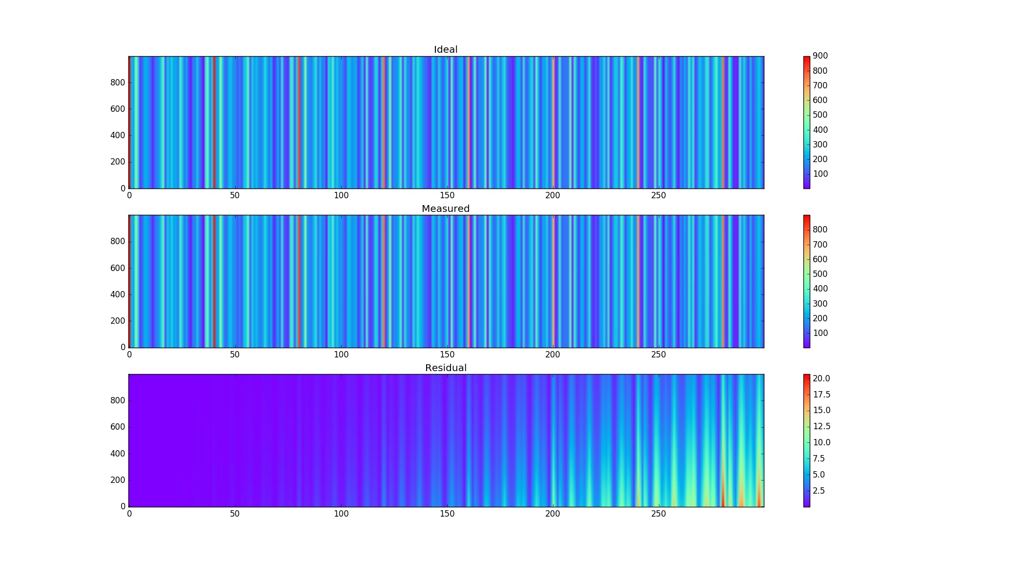
Figure 3 shows simulated results from a distribution of flat-spectrum point sources. The following system parameters were used: signal band in $300$ to $500\;MHz$, spectral resolution of $200\;kHz$, minimum and maximum antenna separations of $x_{min}=1.5$ and $x_{max}=748.5$ meters respectively. The minimum and maximum reference baselines common to all channels are taken to be $u_{min}=x_{min}/\lambda_{min}=2.502$ and $u_{max}=x_{max}/\lambda_{max}=749.018$ respectively. The intermediate baselines are integer multiples of $u_{min}$.

For the channel’s spectral response, a single-block Blackman-Nuttal window with coefficients as specified in Table-2 of Price D. C. (2018), was used. The microtone resolution was set to $200\;Hz$ so that $\sigma=1000$. To simulate the intra-channel effect, visibilities from microtones spanning $\pm 5f_{res}$ around the channel center frequency were weighted by $|H(f-f_{b})|^{2}$ and superposed. For a single point source, the magnitude of residual visibility $|1-G_{u_{0}}(b)|.|V_{u_{0}}(b)|$ is a function of $|l_{0}u_{0}|f_{res}/|f_{b}|$. For the point source distribution, as seen in the third plot, the residual becomes worse as $|u_{0}|$ increases or $|f_{b}|$ decreases.

References

• [1] Chennamangalam J. 2016, online: https://casper.berkeley.edu/wiki/The_Polyphase_Filter_Bank_Technique
• [2] Marthi V. R. et al. 2017, MNRAS, 471, 3112
• [3] Morales M. F. et al. 2012, ApJ, 752, 137
• [4] Parsons A. R. et al. 2012, ApJ, 756, 165
• [5] Price D. C. 2018, arXiv:1607.03579
• [6] Thompson, A. R., Moran, J. M., Swenson, Jr., G. W. 2017, Interferometry and Synthesis in Radio Astronomy, 3rd Edition, Springer, p. 369
• [7] Thyagarajan N. et al. 2013, ApJ, 776, 6
• [8] Thyagarajan N. et al. 2015a, ApJ, 804, 14
• [9] Thyagarajan N. et al. 2015b, ApJ, 807, L28
• [10] Vedantham H. et al. 2012, ApJ, 745, 176