A Nitsche-eXtended finite element method for distributed optimal control problems of elliptic interface equations Thanks: This work was supported by National Natural Science Foundation of China (11771312).

Tao Wang ^†^†thanks: Email: wangtao5233@hotmail.com Chaochao Yang ^†^†thanks: Email: yangchaochao9055@163.com Xiaoping Xie ^†^†thanks: Corresponding author. Email: xpxie@scu.edu.cn Affiliation: School of Mathematics, Sichuan University, Chengdu 610064, China

Abstract

This paper analyzes an interface-unfitted numerical method for distributed optimal control problems governed by elliptic interface equations. We follow the variational discretization concept to discretize the optimal control problems, and apply a Nitsche-eXtended finite element method to discretize the corresponding state and adjoint equations, where piecewise cut basis functions around the interface are enriched into the standard linear element space. Optimal error estimates of the state, co-state and control in a mesh-dependent norm and the $L^{2}$ norm are derived. Numerical results are provided to verify the theoretical results.

Keywords: distributed optimal control, elliptic interface equation, variational discretization concept, interface-unfitted finite element method.

1 Introduction

Optimization processes in multi-physics progress or engineering design with different materials usually lead to optimal control problems governed by partial differential equations with interfaces. In this paper, we consider the following distributed optimal control problem:

\text{min}~J(y,u):=\frac{1}{2}\int_{\Omega}(y-y_{d})^{2}~dx+\frac{\nu}{2}\int_{\Omega}u^{2}~dx

(1.1)

for $(y,u)\in H^{1}_{0}(\Omega)\times L^{2}(\Omega)$ subject to the elliptic interface problem

\left\{\begin{array}[]{rll}&-\nabla\cdot(\alpha(x)\nabla y)=f+u,&\text{ in }\Omega\\ &y=0,&\text{ on }\partial\Omega\\ &[y]=0,[\alpha\nabla_{n}y]=g,&\text{ on }\Gamma\\ \end{array}\right.

(1.2)

with the control constraint

u_{0}\leq u\leq u_{1},\text{ a.e. in }\Omega.

(1.3)

Here $\Omega\subseteq\mathbb{R}^{d}(d=2,3)$ is a polygonal or polyhedral domain, consisting of two disjoint subdomains $\Omega_{i}(1\leq i\leq 2)$ , and interface $\Gamma=\partial\Omega_{1}\cap\partial\Omega_{2}$ . $y_{d}\in L^{2}(\Omega)$ is the desired state to be achieved by controlling $u$ , and $\nu$ is a positive constant. $\alpha(x)$ is piecewise constant with $\alpha|_{\Omega_{i}}=\alpha_{i}>0$ for $i=1,2$ , $[y]:=(y|_{\Omega_{1}})|_{\Gamma}-(y|_{\Omega_{2}})|_{\Gamma}$ is the jump of function $y$ across interface $\Gamma$ , n is the unit normal vector along $\Gamma$ pointing to $\Omega_{1}$ , $\nabla_{\textbf{n}}y=n\cdot\nabla y$ is the normal derivative of $y$ , $f\in L^{2}(\Omega)$ , $g\in L^{2}(\Gamma)$ , and $u_{0},u_{1}\in L^{2}(\Omega)$ with $u_{0}\leq u_{1}$ a.e. in $\Omega$ . The choice of homogeneous boundary condition on boundary $\partial\Omega$ is made for ease of presentation, since similar results are valid for other boundary conditions.

For an elliptic interface problem, it is well-known that its solution is generally not in $H^{2}(\Omega)$ due to the discontinuity of coefficient. This low regularity may lead to reduced accuracy for numerical approximations [2, 47]. In literature there are usually two types of methods to improve the numerical accuracy, interface(or body)-fitted methods [6, 9, 14, 36, 26, 11] and interface-unfitted methods. For the interface-fitted methods, meshes aligned with the interface are used so as to dominate the approximation error caused by the non-smoothness of solution. However, it is often difficult or expensive to generate complicated interface-fitted meshes, especially when the interface is moving with time or iteration.

In contrast with the interface-fitted methods, the interface-fitted methods, with certain types of modification for approximating functions around the interface, can avoid using the interface-fitted meshes. One typical type of interface-unfitted methods is the extended/generalized finite element method ( XFEM/GFEM) (cf. [4, 41, 3, 33, 34]), where additional basis functions characterizing the singularity of solution around the interface are enriched into the corresponding approximation space. We refer to [24, 40, 15] for the numerical simulation of XFEM/GFEM for some elliptic interface problems. The immersed finite element method (IFEM) (cf. [12, 28, 29, 48]) is another typical type of interface-unfitted methods, where special finite element basis functions are constructed to satisfy the homogeneous interface jump conditions in a certain sense. We note that it is usually not easy to extend the IFEM to the case of non-homogeneous interface conditions [48, 20, 17] and, as pointed out in [31], the classic IFEM may lead to deteriorate accuracy, while partially penalized IFEMs, with extra stabilization terms introduced at interface edges for penalizing the discontinuity in IFE functions, are optimally convergent.

In [18], a special XFEM with optimal convergence was proposed for the elliptic interface problems. This method, called Nitsche-XFEM, combines the idea of XFEM with Nitsche’s approach [35], where additional cut basis functions which are discontinuous across the interface are added into the standard linear finite element space, and the parameters in the Nitsche’s numerical fluxes on each element intersected by the interface are chosen to depend on the relative area/volume of the two parts aside the interface. For the development of interface-unfitted methods using additional cut basis functions, we refer to [7, 5, 25, 19, 10, 44].

For optimal control problems governed by elliptic equations with smooth coefficients, a lot of work on finite element methods can be found in literature; see [22, 13, 49, 45, 50] for control constraints, see [32, 21, 37] for state constraints, see [8, 16, 27, 38] for adaptive convergence analysis. However, there are only limited papers on the numerical analysis for optimal control problems of elliptic interface equations. In [51] the classic IFEM was applied to discretize the model (1.1)-(1.3) with the homogeneous interface jump condition $g=0$ . In [43], $hp$ -finite elements were investigated for the optimal control problems of elliptic interface equations on interface-fitted meshes. In a very recent work [49], the Nitsche-XFEM was applied for interface optimal control problems of elliptic interface equations and shown to have optimal convergence.

In this paper, we shall follow the variational discretization concept and apply the Nitsche-XFEM for the numerical solution of the distributed optimal control problem (1.1)-(1.3). Optimal error estimates will be derived for the state, co-state and control on meshes independent of the interface.

The remainder of the paper is organized as following. Section 2 introduces some notations and the optimality conditions for the optimal control problem. Section 3 gives a brief introduction for Nitsche-XFEM and several theoretical results associated with this method. In section 4, we discretize the optimal control problem, show its discrete optimality conditions, and derive error estimates for the state, co-state and control of the optimal control problem. Section 5 describes an iteration algorithm for the discrete system, and Section 6 provides several numerical examples to verify our theoretical results. Finally, Section 7 gives concluding remarks.

2 Notation and optimality conditions

For any bounded domain $\Lambda\subset\mathbb{R}^{d}$ and non-negative integer $j$ , let $H^{j}(\Lambda)$ and $H^{j}_{0}(\Lambda)$ denote the standard Sobolev spaces on $\Lambda$ with norm $\|\cdot\|_{j,\Lambda}$ and semi-norm $|\cdot|_{j,\Lambda}$ . In particular, $L^{2}(\Lambda):=H^{0}(\Lambda)$ , with the standard $L^{2}$ -inner product $(\cdot,\cdot)_{\Lambda}$ . When $\Lambda=\Omega$ , we use abbreviations $\|\cdot\|_{j}:=\|\cdot\|_{j,\Omega}$ , $|\cdot|_{j}:=|\cdot|_{j,\Omega}$ , and $(\cdot,\cdot):=(\cdot,\cdot)_{\Omega}$ . We also need the fractional Sobolev space

H^{j+\frac{1}{2}}(\Lambda):=\{w\in H^{j}(\Lambda):\sum_{|\alpha|=j}\iint_{\Lambda\times\Lambda}\frac{|D^{\alpha}w(s)-D^{\alpha}w(t)|^{2}}{|s-t|^{d+1}}~dsdt<\infty\}

with norm

\|w\|_{j+\frac{1}{2},\Lambda}:=\left(\|w\|_{j,\Lambda}^{2}+\sum_{|\alpha|=j}\iint_{\Lambda\times\Lambda}\frac{|D^{\alpha}w(s)-D^{\alpha}w(t)|^{2}}{|s-t|^{d+1}}~dsdt\right)^{\frac{1}{2}}.

For $s\in\mathbb{R}^{+}$ , we define

H^{s}(\Omega_{1}\cup\Omega_{2}):=\left\{w\in L^{2}(\Omega):\ w|_{\Omega_{i}}\in H^{s}(\Omega_{i}),\ i=1,2\right\}

with norm

\|\cdot\|_{s,\Omega_{1}\cup\Omega_{2}}:=\left(\sum\limits_{i=1}^{2}\|\cdot\|_{s,\Omega_{i}}^{2}\right)^{\frac{1}{2}}.

Throughout this paper, we use $\bar{a}\lesssim\bar{b}$ to denote $\bar{a}\leq C\bar{b}$ , where $C$ is a generic positive constant $C$ independent of the mesh parameter $h$ and the location of the interface relative to the corresponding mesh.

The weak formulation of state equation (3.5) is as follows: find $y\in H^{1}_{0}(\Omega)$ such that

a(y,v)=(u+f,v)+(g,v)_{\Gamma},\quad\forall v\in H^{1}_{0}(\Omega),

(2.1)

where $a(y,v):=(\alpha\nabla y,\nabla v)$ .It is easy to see that problem (2.1) admits a unique solution. We make the following regularity assumptions for the solution $y$ .

Assumption 1.

It holds $y\in H_{0}^{1}(\Omega)\cap H^{3/2}(\Omega_{1}\cup\Omega_{2})$ and

\|y\|_{\frac{3}{2},\Omega_{1}\cup\Omega_{2}}\lesssim\|u\|_{0}+\|f\|_{0}+\|g\|_{0,\Gamma}.

(2.2)

In addition, if $g\in H^{1/2}(\Gamma)$ , then $y\in H_{0}^{1}(\Omega)\cap H^{2}(\Omega_{1}\cup\Omega_{2})$ and

\|y\|_{2,\Omega_{1}\cup\Omega_{2}}\lesssim\|u\|_{0}+\|f\|_{0}+\|g\|_{\frac{1}{2},\Gamma}.

(2.3)

Remark 2.1.

We note that the Assumption 1 is reasonable. In fact, if $\Omega$ and $\Gamma$ are smooth with $\Gamma\cap\partial\Omega=\emptyset$ , then the regularity (2.2) holds [9, (2.2)]. And it has been shown in [43, Corollary 4.12] that (2.2) holds if $\Omega\subset\mathbb{R}^{2}$ and its subdomains $\Omega_{i}$ are all polygonal. As for the regularity (2.3), if the domain $\Omega$ is convex, and the interface $\Gamma$ is $C^{2}$ continuous with $\Gamma\cap\partial\Omega=\emptyset$ , then (2.3) holds [14, theorem 2.1].

Define

U_{ad}:=\{u\in L^{2}(\Omega):u_{a}\leq u\leq u_{b}\ \text{a.e. in}\ \Omega\}.

By using the standard technique in [42], we can easily derive the optimality conditions for the optimal control problem (1.1)-(1.3).

Lemma 2.1.

The optimal control problem (1.1)-(1.3) has a unique solution $(y,u)\in H_{0}^{1}(\Omega)\times U_{ad}$ , and the equivalent optimality conditions read: the triple $(y,p,u)\in H_{0}^{1}(\Omega)\times H_{0}^{1}(\Omega)\times U_{ad}$ satisfies

		$\displaystyle a(y,v)=(u+f,v)+(g,v)_{\Gamma},~~\forall v\in H_{0}^{1}(\Omega),$		(2.4)
		$\displaystyle a(v,p)=(y-y_{d},v),~~\forall v\in H_{0}^{1}(\Omega),$		(2.5)
		$\displaystyle(p+au,v-u)\geq 0,~~\forall v\in U_{ad}.$		(2.6)

Remark 2.2.

$p$ in (2.5) is called the co-state or adjoint state. In addition, by Assumption 1 we have

\|p\|_{2,\Omega_{1}\cup\Omega_{2}}\lesssim\|y\|_{0}+\|y_{d}\|_{0}.

Remark 2.3.

The variational inequality (2.6) means

u=P_{U_{ad}}\left(-\frac{1}{\nu}p\right),

(2.7)

where $P_{U_{ad}}$ is the $L^{2}$ projection onto $U_{ad}$ . In particular, if $u$ is unconstrained, i.e. $U_{ad}=L^{2}(\Omega)$ , then the relation (2.7) is reduced to

u=-\frac{1}{\nu}p.

(2.8)

3 Nitsche-XFEM for state and co-state equations

3.1 Extended finite element space

Let $\mathscr{T}_{h}$ be a shape-regular triangulation of $\Omega$ consisting of open triangles/tetrahedrons with mesh size $h=\max_{T\in\mathscr{T}_{h}}h_{T}$ , where $h_{T}$ denotes the diameter of $T\in\mathscr{T}_{h}$ . We mention that $\mathscr{T}_{h}$ is independent of the location of interface.

Define

\displaystyle\mathcal{T}_{h}^{\Gamma}:=\{T\in\mathscr{T}_{h}:T\cap\Gamma\neq\emptyset\}.

For any $T\in\mathcal{T}_{h}^{\Gamma}$ , called an interface element, we set $T_{m}:=T\cap\Omega_{m}(m=1,2),\Gamma_{T}:=\Gamma\cap T$ , and denote by $\Gamma_{T,h}$ the straight line/plane segment connecting the intersection between $\Gamma$ and $\partial T$ .

For ease of discussion, we make the following standard assumptions on $\mathscr{T}_{h}$ and $\Gamma$ (cf. [18, 39]).

(A1).

For $T\in\mathcal{T}_{h}^{\Gamma}$ and an edge/face $F\subset\partial T$ , $\Gamma\cap F$ is simply connected.
(A2).

For $T\in\mathcal{T}_{h}^{\Gamma}$ , there is a smooth function $\psi$ which maps $\Gamma_{T,h}$ onto $\Gamma_{T}.$

Remark 3.1.

We note that (A1) is easily fulfilled for sufficiently fine meshes, and (A2) requires $\Gamma$ to be piecewise smooth.

Denote by $\Theta:=\{P_{i}:i=1,2,\cdots,I\}$ the set of all mesh points of the triangulation $\mathcal{T}_{h}$ , and by $\Theta_{\Gamma}:=\Theta\bigcap\bar{\mathcal{T}}_{h}^{\Gamma}$ the set of all vertexes of the interface elements. Let $V_{h}^{P}$ be the standard linear finite element space with respect to the triangulation $\mathcal{T}_{h}$ with $\varphi_{i}\in V_{h}^{P}$ denoting the nodal basis function corresponding to the node $P_{i}$ for $i=1,2,\cdots,I$ .

For any $P_{i}\in\Theta_{\Gamma}\bigcap\Omega_{m}$ ( $m=1,2$ ), define the cut basis function $\widetilde{\varphi_{i}}$ by

\widetilde{\varphi_{i}}(x):=\left\{\begin{array}[]{ll}0,&x\in\Omega_{m},\\ \varphi_{i}(x),&x\in\Omega\setminus\Omega_{m}.\end{array}\right.

Then we introduce the cut finite element space

V_{h}^{\Gamma}:=span\{\widetilde{\varphi_{i}}:P_{i}\in\Theta_{\Gamma}\setminus\Gamma\},

and define the extended finite element space

V_{h}:=\{v_{h}\in V_{h}^{P}\oplus V_{h}^{\Gamma}:v_{h}|_{\partial\Omega}=0\}.

It is easy to see that for any $v_{h}\in V_{h}$ , $v_{h}|_{\Omega_{i}}$ ( $i=1,2$ ) is piecewise linear and continuous, and $v_{h}$ is discontinuous across the interface $\Gamma$ .

3.2 Formulations of Nitsche-XFEM

To describe the Nitsche-XFEM, we first introduce some notations. For each interface element $T\in\mathcal{T}_{h}^{\Gamma}$ and $m=1,2$ , we set

T_{m}:=T\bigcap{\Omega_{m}},\quad k_{m}:=\frac{|T_{m}|}{|T|},\

where $|T_{m}|$ and $|T|$ denote the area/volume of $T_{m}$ and $T$ respectively. It is evident that

k_{1}+k_{2}=1.

For $\phi\in V^{h}$ , we set

\phi_{m}:=\phi|_{\Omega_{m}},\quad\{\phi\}:=(k_{1}\phi_{1}+k_{2}\phi_{2})|_{\Gamma}.

Introduce the following bilinear form $a_{h}(\cdot,\cdot)$ : for $w_{h},v_{h}\in V_{h}$ ,

\displaystyle a_{h}(w_{h},v_{h})

\displaystyle:=(\alpha\nabla w_{h},\nabla v_{h})_{\Omega_{1}\cup\Omega_{2}}-(\{\alpha\nabla_{\textbf{n}}w_{h}\},[v_{h}])_{\Gamma}-(\{\alpha\nabla_{\textbf{n}}v_{h}\},[w_{h}])_{\Gamma}+\lambda([w_{h}],[v_{h}])_{\Gamma},

(3.1)

where the stabilization parameter $\lambda$ is taken as

\lambda|_{T}=\widetilde{C}h_{T}^{-1}\max\{\alpha_{1},\alpha_{2}\},

(3.2)

with $\tilde{C}$ a positive constant.

Then, by following [18], the Nitsche-XFEMs for the state equation (2.4) and the co-state equation (2.5) are respectively given as follows.

Find $y^{h}\in V_{h}$ such that

\displaystyle a_{h}(y^{h},v_{h})=(u+f,v_{h})+(k_{2}g,v_{h1})_{\Gamma}+(k_{1}g,v_{h2})_{\Gamma},\quad\forall v_{h}\in V_{h}.

(3.3)

Find $p^{h}\in V_{h}$ such that

a_{h}(v_{h},p^{h})=(y-y_{d},v_{h}),\quad\forall v_{h}\in V_{h}.

(3.4)

Remark 3.2.

Note that the bilinear form $a_{h}(\cdot,\cdot)$ corresponds to the symmetric interior penalty Galerkin (SIPG) method [1, 46].

Remark 3.3.

In the stabilization term $\lambda([w_{h}],[v_{h}])_{\Gamma}$ of $a_{h}(w_{h},v_{h})$ with $\lambda|_{T}=\widetilde{C}h_{T}^{-1}\max\{\alpha_{1},\alpha_{2}\}$ , the positive constant $\widetilde{C}$ is required to be “sufficiently large” to ensure the coercivity of $a_{h}(\cdot,\cdot)$ (cf. (3.9)).

Remark 3.4.

In [44], a “parameter-friendly” DG-XFE scheme was proposed for the following type of interface problem:

\left\{\begin{array}[]{rll}&-\nabla\cdot(\alpha(x)\nabla w)=f&\text{ in }\Omega,\\ &w=0&\text{ on }\partial\Omega,\\ &[w]=g_{D},\ [\alpha\nabla_{n}w]=g_{N}&\text{ on }\Gamma,\\ \end{array}\right.

(3.5)

where the interface $\Gamma$ is assumed to be $C^{2}(\Omega)$ -smooth. Let $p$ be any given positive integer, and set

\tilde{V}_{h}:=\{v_{h}\in H^{1}(\Omega):\ v_{h}|_{T}\in\mathcal{P}_{p}(T),\forall T\in\mathcal{T}_{h}\},

W_{h}:=\chi_{1}\tilde{V}_{h}+\chi_{2}\tilde{V}_{h},

where $\mathcal{P}_{p}(T)$ denotes the set of polynomials of degree no more than $p$ , and $\chi_{m}$ is the characteristic function of $\Omega_{m}$ for $m=1,2$ . Then the DG-XFE is formulated as follows: find $w_{h}\in W_{h}$ such that

	$\displaystyle a^{*}_{h}(w_{h},v_{h})=$	$\displaystyle(f,v_{h})+(k_{2}{g_{N}},v_{h1})_{\Gamma}+(k_{1}{g_{N}},v_{h2})_{\Gamma}-$
		$\displaystyle(g_{D},\{\alpha\nabla_{n}v\})_{\Gamma}+(\lambda_{1}^{}g_{D},[v_{h}])_{\Gamma}+\underset{T\in\mathcal{T}_{h}^{\Gamma}}{\sum}(\lambda^{}_{2}\alpha r_{e}([g_{D}]),r_{e}([v_{h}])),\quad\forall v_{h}\in W_{h}.$

Here

	$\displaystyle a^{*}_{h}(w_{h},v_{h})$	$\displaystyle:=(\alpha\nabla w_{h},\nabla v_{h})_{\Omega_{1}\cup\Omega_{2}}-(\{\alpha\nabla_{\textbf{n}}w_{h}\},[v_{h}])_{\Gamma}-(\{\alpha\nabla_{\textbf{n}}v_{h}\},[w_{h}])_{\Gamma}+$
		$\displaystyle\lambda^{*}([w_{h}],[v_{h}])_{\Gamma}+\underset{T\in\mathcal{T}_{h}^{\Gamma}}{\sum}(\eta\alpha r_{e}([w_{h}]),r_{e}([v_{h}])),$

and, for any $e=T\cap\Gamma$ with $T\in\mathcal{T}_{h}^{\Gamma}$ , $r_{e}:L^{2}(e)^{d}\rightarrow Z_{T}$ is a lifting operator given by

\int_{T}r_{e}(q)\cdot\alpha z_{h}=-\int_{e}q\cdot\{\alpha z_{h}\}\quad\forall z_{h}\in Z_{T},

where

Z_{T}=\{z_{h}\in L^{2}(\Omega)^{d}:z_{h}|_{T_{m}}\in P_{p}(T_{m})^{d},\ z_{h}|_{\Omega\setminus T}=0\}.

As shown in [44], the introduction of the penalization term based on the lifting operator $r_{e}$ locally along the interface guarantees the coercivity of $a^{*}_{h}(\cdot,\cdot)$ as long as the stabilization parameters $\lambda^{*}|_{T}\geq h_{T}^{-1}$ and $\eta\geq 2$ .

Let us introduce a mesh-dependent norm $|||\cdot|||$ on $H^{3/2}(\Omega_{1}\cup\Omega_{2})$ :

|||v|||^{2}:=\|\nabla v\|^{2}_{0,{\Omega_{1}\cup\Omega_{2}}}+\|\{\nabla_{\textbf{n}}v\}\|^{2}_{-1/2,h,\Gamma}+\|[v]\|^{2}_{1/2,h,\Gamma},\quad\forall v\in H^{3/2}(\Omega_{1}\cup\Omega_{2}),

(3.6)

where

\|v\|^{2}_{1/2,h,\Gamma}:=\underset{T\in\mathcal{T}_{h}^{\Gamma}}{\sum}h_{T}^{-1}\|v\|^{2}_{0,\Gamma_{T}},\quad\|v\|^{2}_{-1/2,h,\Gamma}:=\underset{T\in\mathcal{T}_{h}^{\Gamma}}{\sum}h_{T}\|v\|^{2}_{0,\Gamma_{T}}.

It is easy to see that $|||\cdot|||$ is a norm on $V^{h}$ with

||v_{h}||_{0,\Omega}\lesssim|v_{h}|_{1,\Omega_{1}\cup\Omega_{2}}\leq|||v_{h}|||,\quad\forall v_{h}\in V^{h}.

(3.7)

Under the assumptions (A1)-(A2), the following boundedness and coerciveness results hold (cf. [1, 18]):

a_{h}(w,v)\lesssim|||w|||\ |||v|||,\quad\forall w,v\in H^{3/2}(\Omega_{1}\cup\Omega_{2}),

(3.8)

and

a_{h}(v_{h},w_{h})\gtrsim|||v_{h}|||^{2},\quad\forall v_{h}\in V^{h}

(3.9)

if $\tilde{C}$ in (3.2) is sufficiently large. Hence, the discrete problems (3.3) and (3.4) admit unique solutions $y^{h}\in V_{h}$ and $p^{h}\in V_{h}$ , respectively. In addition, from [18, 49] we have the following error estimates.

Lemma 3.1.

[18] Let $y,p\in H^{1}_{0}(\Omega)\cap H^{2}(\Omega_{1}\cup\Omega_{2})$ be the solutions to the weak problems (2.4) and (2.5), respectively. Then it holds

|||y-y^{h}|||\lesssim h\|y\|_{2,\Omega_{1}\cup\Omega_{2}},\quad|||p-p^{h}|||\lesssim h\|p\|_{2,\Omega_{1}\cup\Omega_{2}}.

\|y-y^{h}\|_{0}\lesssim h^{2}\|y\|_{2,\Omega_{1}\cup\Omega_{2}},\quad\|p-p^{h}\|_{0}\lesssim h^{2}\|p\|_{2,\Omega_{1}\cup\Omega_{2}}.

Lemma 3.2.

[49] Let $y,p\in H^{1}_{0}(\Omega)\cap H^{3/2}(\Omega_{1}\cup\Omega_{2})$ be the solutions to the weak problems (2.4) and (2.5), respectively. Then it holds

|||y-y^{h}|||\lesssim h^{\frac{1}{2}}\|y\|_{\frac{3}{2},\Omega_{1}\cup\Omega_{2}},\quad|||p-p^{h}|||\lesssim h^{\frac{1}{2}}\|p\|_{\frac{3}{2},\Omega_{1}\cup\Omega_{2}},

\|y-y^{h}\|_{0,\Omega}\lesssim h\|y\|_{\frac{3}{2},\Omega_{1}\cup\Omega_{2}},\quad\|p-p^{h}\|_{0,\Omega}\lesssim h\|p\|_{\frac{3}{2},\Omega_{1}\cup\Omega_{2}}.

4 Discretization of optimal control problem

4.1 Discrete optimality conditions

By following the variational discretization concept in [22], the optimal control problem (1.1)-(1.3) is approximated by the following discrete optimal control problem:

\min\limits_{(y_{h},u)\in V_{h}\times U_{ad}}J_{h}(y_{h},u)=\frac{1}{2}\int_{\Omega}(y_{h}-y_{d})^{2}dx+\frac{\nu}{2}\int_{\Omega}u^{2}dx

(4.1)

with

a_{h}(y_{h},v_{h})=(u+f,v_{h})+(k_{2}g,v_{h1})_{\Gamma}+(k_{1}g,v_{h2})_{\Gamma},\quad\forall v_{h}\in V_{h}.

(4.2)

Similar to Lemma 2.1, the following lemma holds.

Lemma 4.1.

The discrete optimal control problem (4.1)-(4.2) has a unique solution, and the solution $(y_{h},p_{h},u_{h})\in V_{h}\times V_{h}\times U_{ad}$ satisfies the following optimality conditions:

		$\displaystyle a(y_{h},v_{h})=(u_{h}+f,v_{h})+(k_{2}g,v_{h1})_{\Gamma}+(k_{1}g,v_{h2})_{\Gamma},\quad\forall v_{h}\in V_{h},$		(4.3)
		$\displaystyle a(v_{h},p_{h})=(y_{h}-y_{d},v_{h}),\quad\forall v_{h}\in V_{h},$		(4.4)
		$\displaystyle(p_{h}+au_{h},v-u_{h})\geq 0,\quad\forall v\in U_{ad}.$		(4.5)

Remark 4.1.

Notice that the discrete optimal control $u_{h}\in U_{ad}$ is not directly discretized in the objective functional (4.1), since $U_{ad}$ is infinite dimensional. However, the variational inequality (4.5) means that $u_{h}$ is implicitly discretized through the discrete co-state $p_{h}$ and the projection $P_{U_{ad}}$ (cf. (2.7)) with

u_{h}=P_{U_{ad}}\left(-\frac{1}{\nu}p_{h}\right).

(4.6)

Moreover, if $u_{0}$ and $u_{1}$ are well-defined at any $x\in\Omega$ , then (4.6) is equivalent to

u_{h}=\min\left\{u_{1},\max\left\{u_{0},-\frac{1}{\nu}p_{h}\right\}\right\}.

(4.7)

In particular, if $U_{ad}=L^{2}(\Omega)$ , then we have

u_{h}=-\frac{1}{\nu}p_{h}.

(4.8)

4.2 Error estimates

In this subsection, we first show that the errors between $(y,p,u)$ and $(y_{h},p_{h},u_{h})$ , the solutions to the continuous optimal control problem (2.4)-(2.6) and to the discrete optimal control problem (4.3)-(4.5) respectively, can be bounded from above by the errors between $(y,p)$ and $(y^{h},p^{h})$ . Here we recall that $y^{h}\in V_{h}$ and $p^{h}\in V_{h}$ are the solutions to the Nitsche-XFE schemes (3.3) and (3.4), respectively.

Theorem 4.1.

Let $(y,p,u)\in H_{0}^{1}(\Omega)\times H_{0}^{1}(\Omega)\times U_{ad}$ and $(y_{h},p_{h},u_{h})\in V_{h}\times V_{h}\times U_{ad}$ be the solutions to the continuous problem (2.4)-(2.6) and the discrete problem (4.3)-(4.5), respectively. Then we have

$\displaystyle\nu^{\frac{1}{2}}\\|u-u_{h}\\|_{0}+\\|y-y_{h}\\|_{0}$	$\displaystyle\lesssim$	$\displaystyle\\|y-y^{h}\\|_{0}+{\nu^{-\frac{1}{2}}}\\|p-p^{h}\\|_{0},$	(4.9)
$\displaystyle\\|p-p_{h}\\|_{0}$	$\displaystyle\lesssim$	$\displaystyle\\|p-p^{h}\\|_{0}+\\|y-y_{h}\\|_{0},$	(4.10)
$\displaystyle\|\|\|y-y_{h}\|\|\|$	$\displaystyle\lesssim$	$\displaystyle\|\|\|y-y^{h}\|\|\|+\\|u-u_{h}\\|_{0},$	(4.11)
$\displaystyle\|\|\|p-p_{h}\|\|\|$	$\displaystyle\lesssim$	$\displaystyle\|\|\|p-p^{h}\|\|\|+\\|y-y_{h}\\|_{0}.$	(4.12)

Proof.

First, by (4.3)-(4.4) and (3.3)-(3.4) we have

	$\displaystyle a_{h}(y_{h}-y^{h},v_{h})$	$\displaystyle=(u_{h}-u,v_{h}),\quad\forall v_{h}\in V_{h},$		(4.13)
	$\displaystyle a_{h}(v_{h},p_{h}-p^{h})$	$\displaystyle=(y_{h}-y,v_{h}),\quad\forall v_{h}\in V_{h},$		(4.14)

which yield

\displaystyle(y_{h}-y,y_{h}-y^{h})

\displaystyle=a_{h}(y_{h}-y^{h},p_{h}-p^{h})=(u_{h}-u,p_{h}-p^{h}).

(4.15)

Take $v=u_{h}$ in (2.6) and $v=u$ in (4.5), we get

	$\displaystyle(\nu u+p,u_{h}-u)$	$\displaystyle\geq 0,$
	$\displaystyle(\nu u_{h}+p_{h},u-u_{h})$	$\displaystyle\geq 0.$

Adding together these two inequalities implies

(\nu(u-u_{h})+p-p_{h},u_{h}-u)\geq 0,

which, together with (4.15), leads to

	$\displaystyle\nu\\|u-u_{h}\\|^{2}_{0}$	$\displaystyle\leq(u_{h}-u,p-p_{h})$
		$\displaystyle=(u_{h}-u,p-p^{h})+(u_{h}-u,p^{h}-p_{h})$
		$\displaystyle=(u_{h}-u,p-p^{h})+(y_{h}-y,y^{h}-y_{h})$
		$\displaystyle\leq\frac{1}{2}(\nu\\|u_{h}-u\\|^{2}_{0}+\frac{1}{\nu}\\|p-p^{h}\\|^{2}_{0})+(y_{h}-y,y^{h}-y_{h})$
		$\displaystyle\leq\frac{1}{2}(\nu\\|u_{h}-u\\|^{2}_{0}+\frac{1}{\nu}\\|p-p^{h}\\|^{2}_{0})-\frac{1}{2}\\|y-y_{h}\\|_{0}^{2}+\frac{1}{2}\\|y-y^{h}\\|_{0}^{2}.$

Consequently, (4.9) holds.

Second, let us show (4.10) and (4.11). From (3.7), (3.9) and (4.14), we have

	$\displaystyle\|\|p_{h}-p^{h}\|\|^{2}_{0}$	$\displaystyle\lesssim\|\|\|p_{h}-p^{h}\|\|\|^{2}$
		$\displaystyle\lesssim a_{h}(p_{h}-p^{h},p_{h}-p^{h})=(y_{h}-y,p_{h}-p^{h})$
		$\displaystyle\lesssim\|\|y_{h}-y\|\|_{0}\|\|p_{h}-p^{h}\|\|_{0}$
		$\displaystyle\lesssim\|\|y_{h}-y\|\|_{0}\|\|\|p_{h}-p^{h}\|\|\|,$

which, together with the triangle inequality, yields

	$\displaystyle\\|p-p_{h}\\|_{0}$	$\displaystyle\leq\\|p-p^{h}\\|_{0}+\\|p^{h}-p_{h}\\|_{0}\lesssim\\|p-p^{h}\\|_{0}+\\|y_{h}-y\\|_{0},$
	$\displaystyle\|\|\|p-p_{h}\|\|\|$	$\displaystyle\leq\|\|\|p-p^{h}\|\|\|+\|\|\|p^{h}-p_{h}\|\|\|\lesssim\|\|\|p-p^{h}\|\|\|+\\|y_{h}-y\\|_{0},$

i.e. (4.10) and (4.11) hold.

Similarly, (4.11) follows from (3.7), (3.9) and (4.13). ∎

Based on Theorem 4.1, Lemmas 3.1-3.2, and Remarks 2.3 and 4.1, we immediately have the following main results of error estimation.

Theorem 4.2.

Let $(y,p,u)\in\left(H_{0}^{1}(\Omega)\cap H^{s}(\Omega_{1}\cup\Omega_{2})\right)\times\left(H_{0}^{1}(\Omega)\cap H^{s}(\Omega_{1}\cup\Omega_{2})\right)\times U_{ad}$ ( $s=2,3/2$ ) and $(y_{h},p_{h},u_{h})\in V_{h}\times V_{h}\times U_{ad}$ be the solutions to the continuous problem (2.4)-(2.6) and the discrete problem (4.3)-(4.5), respectively. Then we have, for $s=2$ ,

	$\displaystyle\\|u-u_{h}\\|_{0}+\\|y-y_{h}\\|_{0}+\\|p-p_{h}\\|_{0}$	$\displaystyle\lesssim$	$\displaystyle h^{2}(\\|y\\|_{2,\Omega_{1}\cup\Omega_{2}}+\\|p\\|_{2,\Omega_{1}\cup\Omega_{2}}),$		(4.16)
	$\displaystyle\|\|\|y-y_{h}\|\|\|+\|\|\|p-p_{h}\|\|\|$	$\displaystyle\lesssim$	$\displaystyle h(\\|y\\|_{2,\Omega_{1}\cup\Omega_{2}}+\\|p\\|_{2,\Omega_{1}\cup\Omega_{2}}),$		(4.17)

and for $s=3/2$ ,

	$\displaystyle\\|u-u_{h}\\|_{0}+\\|y-y_{h}\\|_{0}+\\|p-p_{h}\\|_{0}$	$\displaystyle\lesssim$	$\displaystyle h(\\|y\\|_{\frac{3}{2},\Omega_{1}\cup\Omega_{2}}+\\|p\\|_{\frac{3}{2},\Omega_{1}\cup\Omega_{2}}),$		(4.18)
	$\displaystyle\|\|\|y-y_{h}\|\|\|+\|\|\|p-p_{h}\|\|\|$	$\displaystyle\lesssim$	$\displaystyle h^{\frac{1}{2}}(\\|y\\|_{\frac{3}{2},\Omega_{1}\cup\Omega_{2}}+\\|p\\|_{\frac{3}{2},\Omega_{1}\cup\Omega_{2}}).$		(4.19)

In particular, if $u$ is unconstrained, i.e. $U_{ad}=L^{2}(\Omega)$ , then we further have

\displaystyle|||u-u_{h}|||

\displaystyle\lesssim

\displaystyle h^{s-1}(\|y\|_{s,\Omega_{1}\cup\Omega_{2}}+\|p\|_{s,\Omega_{1}\cup\Omega_{2}}),\quad s=2,3/2.

(4.20)

Remark 4.2.

In view of the definition of $|||\cdot|||$ in (3.6), the estimates (4.17) and (4.19) indicate

\displaystyle|y-y_{h}|_{1}+|p-p_{h}|_{1}

\displaystyle\lesssim

\displaystyle h^{s-1}(\|y\|_{s,\Omega_{1}\cup\Omega_{2}}+\|p\|_{s,\Omega_{1}\cup\Omega_{2}}),\quad s=2,3/2,

(4.21)

and (4.20) indicates

\displaystyle|u-u_{h}|_{1}

\displaystyle\lesssim

\displaystyle h^{s-1}(\|y\|_{s,\Omega_{1}\cup\Omega_{2}}+\|p\|_{s,\Omega_{1}\cup\Omega_{2}}),\quad s=2,3/2,

(4.22)

where $|\cdot|_{1}:=|\cdot|_{1,\Omega_{1}\cup\Omega_{2}}.$

5 Numerical results

We shall provide several 2D numerical examples to verify the performance of the Nitsche-XFEM. Note that the optimal control problem (1.1)-(1.2) without the constraint (1.3) is a linear problem, the resultant discrete linear system is easy to solve. However, for the constrained optimal control problem (1.1)-(1.3), the corresponding discrete optimal control problem (4.1)-(4.2) or its equivalent problem (4.3)-(4.5) is a nonlinear system, which we shall apply the following fixed-point iteration algorithm to solve.

Algorithm

Fixed-point iteration

1.

Initialize $u^{i}_{h}=u^{0}$ ;
2.

Compute $y^{i}_{h}\in V_{h}$ by $a_{h}(y_{h}^{i},v_{h})=(u_{h}^{i},v_{h})+(f,v_{h})+(k_{2}g,v_{1,h})_{\Gamma_{h}}+(k_{1}g,v_{2,h})_{\Gamma_{h}},\forall v_{h}\in V_{h}$ ;
3.

Compute $p_{h}^{i}\in V_{h}$ by $a_{h}(v_{h},p_{h}^{i})=(y_{h}^{i}-y_{d},v_{h}),\forall v_{h}\in V_{h}$ ;
4.

Set $u_{h}^{i+1}=\min\left\{u_{1},\max\left\{u_{0},-\frac{1}{\nu}p_{h}^{i}\right\}\right\};$
5.

if $|u_{h}^{i+1}-u_{h}^{i}|<\text{Tol}$ or $i+1>\text{MaxIte}$ , then output $u_{h}=u_{h}^{i+1}$ , else $i=i+1$ , and go back to Step 2.

Here $u^{0}$ is an initial value, Tol is the tolerance, and MaxIte is the maximal iteration number. Theoretically, this algorithm is convergent when the regularity parameter $\nu$ is large enough (cf. [23]).

In each example, we choose $\Omega$ to be a square, and use $N\times N$ uniform meshes with $2N^{2}$ triangular elements.

Example 5.1.

Segment interface: a case without control constraints

Consider the optimal control problem (1.1)-(1.2) without the constraint (1.3). Set the regulation parameter $\nu=0.01$ , the domain $\Omega:=[0,1]\times[0,1]$ (cf. Figure 1), the interface

\Gamma:=\{(x_{1},x_{2}):x_{2}=kx_{1}+b\}\cap\Omega

with $k=-\sqrt{3}/3,b=(6+\sqrt{6}-2\sqrt{3})/6$ , and

\Omega_{1}:=\{(x_{1},x_{2}):kx_{1}+b-x_{2}>0\}\cap\Omega,\quad\Omega_{2}:=\{(x_{1},x_{2}):kx_{1}+b-x_{2}<0\}\cap\Omega.

Take the coefficients $\alpha|_{\Omega_{1}}=\alpha_{1}:=1,\ \alpha|_{\Omega_{2}}=\alpha_{2}:=100$ , and the control space $U_{ad}:=L^{2}(\Omega)$ . Let $y_{d},f,g$ be such that the optimal triple $(y,p,u)$ of (2.4)-(2.6) is of the the following form:

$\displaystyle y(x_{1},x_{2})$	$\displaystyle=$	$\displaystyle\begin{cases}\frac{(x_{2}-kx_{1}-b)cos(x_{1}x_{2})}{2\alpha_{1}}+(x_{2}-kx_{1}-b)^{3},&\mbox{ in $\Omega_{1}$, }\\ \frac{(x_{2}-kx_{1}-b)cos(x_{1}x_{2})}{2\alpha_{2}},&\mbox{ in $\Omega_{2}$, }\end{cases}$
$\displaystyle u(x_{1},x_{2})$	$\displaystyle=$	$\displaystyle\begin{cases}\alpha_{2}(x_{2}-kx_{1}-b)x_{1}(x_{1}-1)x_{2}(x_{2}-1)sin(x_{1}x_{2}),&\mbox{ in $\Omega_{1}$, }\\ \alpha_{1}(x_{2}-kx_{1}-b)x_{1}(x_{1}-1)x_{2}(x_{2}-1)sin(x_{1}x_{2}),&\mbox{ in $\Omega_{2}$, }\end{cases}$
$\displaystyle p(x_{1},x_{2})$	$\displaystyle=$	$\displaystyle-\nu u(x_{1},x_{2}).$

We compute the discrete schemes (4.3)-(4.5) with the stabilization parameter $\widetilde{C}=10$ (cf. (3.2)). Tables 1-2 give numerical results of the relative errors between $(y_{h},p_{h},u_{h})$ and $(y,p,u)$ in the $L^{2}-$ norm and the $H^{1}$ -seminorm, respectively. We can see that the Nitsche-XFEM yields optimal convergence orders, i.e. second order rates of convergence for $|y-y_{h}|_{0}$ , $|p-p_{h}|_{0}$ and $|u-u_{h}|_{0}$ , and first order rates of convergence for $|y-y_{h}|_{1}$ , $|p-p_{h}|_{1}$ and $|u-u_{h}|_{1}$ . This is consistent with our theoretical results in Theorem 4.1.

Refer to caption — Figure 1: Segment interface and $8\times 8$ mesh for Example 5.1

Table 1: Relative errors of Nitsche-XFEM in

L^{2}

-norm for Example 5.1.

N	$\frac{\\|u-u_{h}\\|_{0}}{\\|u\\|_{0}}$	order	$\frac{\\|y-y_{h}\\|_{0}}{\\|y\\|_{0}}$	order	$\frac{\\|p-p_{h}\\|_{0}}{\\|p\\|_{0}}$	order
16	3.9941e-02		8.7667e-03		3.9941e-02
32	9.6399e-03	2.1	2.1955e-04	2.0	9.6399e-03	2.1
64	2.3780e-03	2.0	5.5005e-04	2.0	2.3780e-03	2.0
128	5.9194e-04	2.0	1.3834e-05	2.0	5.9195e-04	2.0
256	1.4794e-04	2.0	3.5203e-06	2.0	1.4794e-04	2.0

Table 2: Relative errors of Nitsche-XFEM in

H^{1}

-seminorm for Example 5.1.

N	$\frac{\|u-u_{h}\|_{1}}{\|u\|_{1}}$	order	$\frac{\|y-y_{h}\|_{1}}{\|y\|_{1}}$	order	$\frac{\|p-p_{h}\|_{1}}{\|p\|_{1}}$	order
16	2.0695e-01		1.0180e-01		2.0695e-01
32	1.0404e-01	1.0	5.0958e-02	1.0	1.0404e-01	1.0
64	5.2064e-02	1.0	2.5486e-02	1.0	5.2064e-02	1.0
128	2.6035e-02	1.0	1.2744e-02	1.0	2.6035e-02	1.0
256	1.3017e-02	1.0	6.3722e-03	1.0	1.3017e-02	1.0

Example 5.2.

Circle interface: a case without control constraints

This example is from [51], where it was used to test the performance of an IFEM. In the optimal control problem (1.1)-(1.2), take $\nu=0.01$ and $\Omega=[-1,1]\times[-1,1]$ . The interface $\Gamma$ is a circle centered at $(0,0)$ with radius $r=\frac{1}{2}$ . Set

\Omega_{1}:=\{(x_{1},x_{2}):x_{1}^{2}+x_{2}^{2}<r^{2}\},\quad\Omega_{2}:=\{(x_{1},x_{2}):x_{1}^{2}+x_{2}^{2}>r^{2}\}\cap\Omega,

$\alpha|_{\Omega_{1}}=\alpha_{1}:=1,\ \alpha|_{\Omega_{2}}=\alpha_{2}:=10$ , and $U_{ad}:=L^{2}(\Omega)$ . Let $y_{d},f,g$ be such that the optimal triple $(y,p,u)$ of (2.4)-(2.6) is of the the following form:

$\displaystyle y(x_{1},x_{2})$	$\displaystyle=$	$\displaystyle\begin{cases}\frac{(x_{1}^{2}+x_{2}^{2})^{\frac{3}{2}}}{\alpha_{1}},&\mbox{ in $\Omega_{1}$ },\\ \frac{(x_{1}^{2}+x_{2}^{2})^{\frac{3}{2}}}{\alpha_{2}}+(\frac{1}{\alpha_{1}}-\frac{1}{\alpha_{2}})r^{3},&\mbox{ in $\Omega_{2}$ },\end{cases}$
$\displaystyle u(x_{1},x_{2})$	$\displaystyle=$	$\displaystyle\begin{cases}\frac{5(x_{1}^{2}+x_{2}^{2}-r^{2})(x_{1}^{2}-1)(x_{2}^{2}-1)}{\alpha_{1}},&\mbox{ in $\Omega_{1}$ },\\ \frac{5(x_{1}^{2}+x_{2}^{2}-r^{2})(x_{1}^{2}-1)(x_{2}^{2}-1)}{\alpha_{2}},&\mbox{ in $\Omega_{2}$ },\end{cases}$
$\displaystyle p(x_{1},x_{2})$	$\displaystyle=$	$\displaystyle-\nu u(x_{1},x_{2}).$

Notice that $g=0$ in this example.

In the schemes (4.3)-(4.5) we take the stabilization parameter $\widetilde{C}=1000$ , and use the polygonal line $\Gamma_{h}=\bigcup\limits_{T\in\mathcal{T}_{h}}\Gamma_{T,h}$ to replace the exact interface $\Gamma$ . Tables 3-4 give some numerical results of the errors in the $L^{2}-$ norm and the $H^{1}$ -seminorm, respectively. For comparison we also list the results from [51] obtained by the classical IFEM. We can see that the Nitsche-XFEM yields optimal convergence orders for all the $L^{2}$ and $H^{1}$ errors. In particular, the convergence rates of Nitsche-XFEM are always full when the mesh is refined, while the rates of IFEM may deteriorate, e.g. the rate of $|u-u_{h}|_{1}$ deteriorates from $1.01$ at the $32\times 32$ mesh to $0.91$ at the $256\times 256$ mesh. In fact, such phenomenon of accuracy deterioration for IFEM has been observed in [30] for elliptic interface problems.

Table 3:

L^{2}

errors of Nitsche-XFEM (abbr. NXFEM) and IFEM for Example 5.2.

Method	N	$\\|u-u_{h}\\|_{0}$	order	$\\|y-y_{h}\\|_{0}$	order	$\\|p-p_{h}\\|_{0}$	order
	16	1.1316e-02		4.4535e-03		1.1316e-04
	32	3.0688e-03	1.88	1.1883e-03	1.91	3.0688e-05	1.88
NXFEM	64	7.5979e-04	2.01	3.1686e-04	1.91	7.5979e-06	2.01
	128	1.8516e-04	2.04	7.6393e-05	2.05	1.8516e-06	2.04
	256	4.2966e-05	2.11	1.8584e-05	2.04	4.2966e-07	2.11
	16	1.1889e-02		4.6400e-03		1.1889e-04
	32	3.1406e-03	1.92	1.2288e-03	1.91	3.1406e-05	1.92
IFEM[51]	64	7.0663e-04	2.15	3.1438e-04	1.96	7.0663e-06	2.15
	128	1.6334e-04	2.11	8.1934e-05	1.93	1.6334e-06	2.11
	256	3.5894e-05	2.18	2.1650e-05	1.92	3.5894e-07	2.18

Table 4:

H^{1}

errors of Nitsche-XFEM and IFEM for Example 5.2.

Method	N	$\|u-u_{h}\|_{1}$	order	$\|y-y_{h}\|_{1}$	order	$\|p-p_{h}\|_{1}$	order
	16	1.1407e-01		1.1311e-01		1.1401e-03
	32	5.7015e-02	1.00	5.8796e-02	0.94	5.6926e-04	1.00
NXFEM	64	2.7869e-02	1.03	2.9448e-02	1.00	2.7932e-04	1.03
	128	1.3830e-02	1.01	1.4800e-02	0.99	1.3852e-04	1.01
	256	6.8465e-03	1.01	7.3659e-03	1.00	6.8465e-05	1.01
	16	1.0665e-01		1.0778e-01		1.0665e-03
	32	5.2602e-02	1.01	5.5660e-02	0.95	5.2602e-04	1.01
IFEM[51]	64	2.7054e-02	0.95	2.9084e-02	0.93	2.7054e-04	0.95
	128	1.4028e-02	0.94	1.5047e-02	0.95	1.4028e-04	0.94
	256	7.4170e-03	0.91	7.9081e-03	0.92	7.4170e-05	0.91

Example 5.3.

Circle Interface: a case with control constraints

Consider the optimal control problem (1.1)-(1.3) with $\nu=1$ and $\Omega=[-1,1]\times[-1,1]$ (cf. Figure 2). The interface $\Gamma$ is a circle centered at $(0,0)$ with radius $r=\frac{\sqrt{3}}{4}$ . Set

\Omega_{1}:=\{(x_{1},x_{2}):x_{1}^{2}+x_{2}^{2}<r^{2}\},\quad\Omega_{2}:=\{(x_{1},x_{2}):x_{1}^{2}+x_{2}^{2}>r^{2}\}\cap\Omega,

$\alpha|_{\Omega_{1}}=\alpha_{1}:=1,\ \alpha|_{\Omega_{2}}=\alpha_{2}:=1000$ , and $U_{ad}:=\{u\in L^{2}(\Omega):-\frac{1}{2}\leq u\leq\frac{1}{2}\ \text{ a.e in}\ \Omega\}$ . Let $y_{d},f,g$ be such that the optimal triple $(y,p,u)$ of (2.4)-(2.6) is of the the following form:

$\displaystyle y(x_{1},x_{2})$	$\displaystyle=$	$\displaystyle\begin{cases}\frac{(x_{1}^{2}+x_{2}^{2})^{\frac{3}{2}}}{\alpha_{1}}-10(x_{1}^{2}+x_{2}^{2}-r^{2})sin(x_{1}x_{2}),&\mbox{ in $\Omega_{1}$ }\\ \frac{(x_{1}^{2}+x_{2}^{2})^{\frac{3}{2}}}{\alpha_{2}}+(\frac{1}{\alpha_{1}}-\frac{1}{\alpha_{2}})r^{3},&\mbox{ in $\Omega_{2}$, }\end{cases}$
$\displaystyle u(x_{1},x_{2})$	$\displaystyle=$	$\displaystyle\min\left\{\frac{1}{2},\max\left\{-\frac{1}{2},\varphi(x_{1},x_{2})\right\}\right\},$
$\displaystyle p(x_{1},x_{2})$	$\displaystyle=$	$\displaystyle-\nu\varphi(x_{1},x_{2}),$

where

\displaystyle\varphi(x_{1},x_{2}):=\begin{cases}\frac{5(x_{1}^{2}+x_{2}^{2}-r^{2})(x_{1}^{2}-1)(x_{2}^{2}-1)}{\alpha_{1}},&\mbox{ in $\Omega_{1}$ }\\ \frac{5(x_{1}^{2}+x_{2}^{2}-r^{2})(x_{1}^{2}-1)(x_{2}^{2}-1)}{\alpha_{2}},&\mbox{ in $\Omega_{2}$ }.\end{cases}

In the schemes (4.3)-(4.5) we take the stabilization parameter $\widetilde{C}=5$ . Tables 5-6 give some numerical results of the relative errors in the $L^{2}-$ norm and the $H^{1}$ -seminorm, respectively. We can see that the NXFEM yields second order rates of convergence for $|y-y_{h}|_{0}$ , $|p-p_{h}|_{0}$ and $|u-u_{h}|_{0}$ , and first order rates of convergence for $|y-y_{h}|_{1}$ and $|p-p_{h}|_{1}$ . This is consistent with Theorem 4.1.

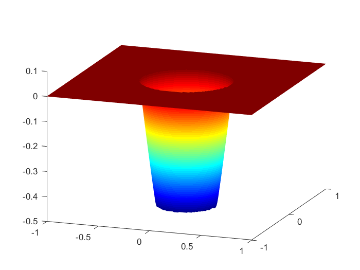
In Figures 3-4 we show the exact solutions of the control $u$ and state $p$ , and the Nitsche-XFEM solutions $u_{h}$ and $p_{h}$ at the 32 $\times$ 32 mesh. Figure 5 demonstrates the boundaries of the exact and the computed active sets. We can see that all the numerical approximations match the exact solutions well.

Table 5: Relative errors of Nitsche-XFEM in

L^{2}

-norm for Example 5.3.

N	$\frac{\\|u-u_{h}\\|_{0}}{\\|u\\|_{0}}$	order	$\frac{\\|y-y_{h}\\|_{0}}{\\|y\\|_{0}}$	order	$\frac{\\|p-p_{h}\\|_{0}}{\\|p\\|_{0}}$	order
16	4.4640e-02		6.7792e-02		5.9076e-02
32	1.7953e-02	1.3	2.3134e-02	1.6	1.8254e-02	1.7
64	3.9458e-03	2.2	5.7710e-03	2.0	3.9865e-03	2.2
128	7.7806e-04	2.3	1.3023e-03	2.2	8.2130e-04	2.3
256	1.2751e-04	2.6	2.0961e-04	2.6	1.5615e-04	2.4

Table 6: Relative errors of Nitsche-XFEM in

H^{1}

-seminorm for Example 5.3.

N	$\frac{\|y-y_{h}\|_{1}}{\|y\|_{1}}$	order	$\frac{\|p-p_{h}\|_{1}}{\|p\|_{1}}$	order
16	5.0048e-01		2.0831e-01
32	2.4468e-01	1.0	1.0421e-01	1.0
64	1.1515e-01	1.1	4.9146e-02	1.1
128	5.7116e-02	1.0	2.4365e-02	1.0
256	2.6058e-02	1.1	1.1514e-02	1.1

6 Conclusion

In this paper, the Nitsche eXtended finite element method as well as the variational discretization concept has been applied to discretize the distributed optimal control problems of elliptic interface equations. This method does not require interface-fitted meshes, and is suitable for generic interface conditions. Error analysis and numerical results have demonstrated its optimal convergence and good performance.

References

[1] Douglas N Arnold. An interior penalty finite element method with discontinuous elements. SIAM Journal on Numerical Analysis, 19(4):742–760, 1982.
[2] Ivo Babuška. The finite element method for elliptic equations with discontinuous coefficients. Computing, 5(3):207–213, 1970.
[3] Ivo Babuška and Uday Banerjee. Stable generalized finite element method (SGFEM). Computer Methods in Applied Mechanics and Engineering, pages 91–111, 2012.
[4] Ivo Babuška, Gabriel Caloz, and John E. Osborn. Special finite element methods for a class of second order elliptic problems with rough coefficients. Siam Journal on Numerical Analysis, 31(4):945–981, 1994.
[5] Nelly Barrau, Roland Becker, Eric Dubach, and Robert Luce. A robust variant of NXFEM for the interface problem. Comptes Rendus Mathematique, 350(15-16):789–792, 2012.
[6] John W. Barrett and Charles M. Elliott. Fitted and unfitted finite-element methods for elliptic equations with smooth interfaces. Ima Journal of Numerical Analysis, 7(3):283–300, 1987.
[7] Roland Becker, Erik Burman, and Peter Hansbo. A nitsche extended finite element method for incompressible elasticity with discontinuous modulus of elasticity. Computer Methods in Applied Mechanics $\&$ Engineering, 198(41–44):3352–3360, 2009.
[8] Roland Becker, Hartmut Kapp, and Rolf Rannacher. Adaptive finite element methods for optimal control of partial differential equations: Basic concept, 2000.
[9] James H. Bramble and J. Thomas King. A finite element method for interface problems in domains with smooth boundaries and interfaces. Advances in Computational Mathematics, 6(1):109–138, 1996.
[10] Erik Burman, Susanne Claus, Peter Hansbo, Mats G Larson, and Andre Massing. Cutfem: Discretizing geometry and partial differential equations. International Journal for Numerical Methods in Engineering, 104(7):472–501, 2015.
[11] Zhiqiang Cai, Cuiyu He, and Shun Zhang. Discontinuous finite element methods for interface problems: Robust a priori and a posteriori error estimates. SIAM Journal on Numerical Analysis, 55(1):400–418, 2017.
[12] Brian Camp, Tao Lin, Yanping Lin, and Weiwei Sun. Quadratic immersed finite element spaces and their approximation capabilities. Advances in Computational Mathematics, 24:81–112, 2006.
[13] Yanping Chen, Yunqing Huang, Wenbin Liu, and Ningning Yan. Error estimates and superconvergence of mixed finite element methods for convex optimal control problems. Journal of Scientific Computing, 42(3):382–403, 2010.
[14] Zhiming Chen and Jun Zou. Finite element methods and their convergence for elliptic and parabolic interface problems. Numerische Mathematik, 79(2):175–202, 1998.
[15] Kwok Wah Cheng and Thomas Peter Fries. Higher‐order xfem for curved strong and weak discontinuities. International Journal for Numerical Methods in Engineering, 82(5):564–590, 2010.
[16] Wei Gong and Ninging Yan. Adaptive finite element method for elliptic optimal control problems: convergence and optimality. Numerische Mathematik., 135(4):1121–1170, 2017.
[17] Daoru Han, Pu Wang, Xiaoming He, Tao Lin, and Joseph Wang. A 3d immersed finite element method with non-homogeneous interface flux jump for applications in particle-in-cell simulations of plasma–lunar surface interactions ☆. Journal of Computational Physics, 321:965–980, 2016.
[18] Anita Hansbo and Peter Hansbo. An unfitted finite element method, based on nitsche’s method, for elliptic interface problems. Computer Methods in Applied Mechanics Engineering, 191(47–48):5537–5552, 2002.
[19] Peter Hansbo, Mats G Larson, and Sara Zahedi. A cut finite element method for a stokes interface problem. Applied Numerical Mathematics, 85:90–114, 2014.
[20] Xiaoming He, Tao Lin, and Yanping Lin. Immersed finite element methods for elliptic interface problems with non-homogeneous jump conditions. International Journal of Numerical Analysis $\&$ Modeling, 8(2):284–301, 2011.
[21] Michael Hintermuller and Ronald H W Hoppe. Goal-oriented adaptivity in pointwise state constrained optimal control of partial differential equations. Siam Journal on Control and Optimization, 48(8):5468–5487, 2010.
[22] Michael Hinze. A variational discretization concept in control constrained optimization: the linear-quadratic case. Computational Optimization and Applications, 30(1):45–61, 2005.
[23] Michael Hinze, Rene Pinnau, Michael Ulbrich, and Stefan Ulbrich. Optimization with PDE Constraints. Springer Netherlands, 2009.
[24] Kenan Kergrene, Ivo Babuška, and Uday Banerjee. Stable generalized finite element method and associated iterative schemes; application to interface problems. Computer Methods in Applied Mechanics $\&$ Engineering, 305:1–36, 2016.
[25] Christoph Lehrenfeld and Arnold Reusken. Analysis of a dg-xfem discretization for a class of two-phase mass transport problems. Siam Journal on Numerical Analysis, 52(52):958–983, 2012.
[26] Jingzhi Li, Jens Markus Melenk, Barbara I Wohlmuth, and Jun Zou. Optimal a priori estimates for higher order finite elements for elliptic interface problems. Applied Numerical Mathematics, 60(1):19–37, 2010.
[27] Ruo Li, Wenbin Liu, Heping Ma, and Tao Tang. Adaptive finite element approximation for distributed elliptic optimal control problems. Siam Journal on Control $\&$ Optimization, 41(5):1321–1349, 2002.
[28] Zhilin Li and Kazufumi Ito. The Immersed Interface Method: Numerical Solutions of PDEs Involving Interfaces and Irregular Domains (Frontiers in Applied Mathematics). Society for Industrial and Applied Mathematics, 2006.
[29] Tao Lin, Yanping Lin, and Weiwei Sun. Error estimation of a class of quadratic immersed finite element methods for elliptic interface problems. Discrete and Continuous Dynamical Systems-series B, 7(4):807–823, 2007.
[30] Tao Lin, Yanping Lin, and Xu Zhang. Partially penalized immersed finite element methods for elliptic interface problems. SIAM Journal on Numerical Analysis, 53(2):1121–1144, 2015.
[31] Tao Lin, Qing Yang, and Xu Zhang. Partially penalized immersed finite element methods for parabolic interface problems. Numerical Methods for Partial Differential Equations, 31(6):1925–1947, 2015.
[32] Wenbin Liu, Wei Gong, and Ninging Yan. A new finite element approximation of a state-constained optimal control problem. Journal of Computational Mathematics, 27(1):97–114, 2009.
[33] Nicolas Möes, John E. Dolbow, and Ted Belytschko. A finite element method for crack growth without remeshing. International Journal for Numerical Methods in Engineering, 46(1):131–150, 1999.
[34] Serge Nicaise, Yves Renard, and Elie Chahine. Optimal convergence analysis for the extended finite element method. International Journal for Numerical Methods in Engineering, 86(4‐5):528–548, 2011.
[35] J. Nitsche. Über ein variationsprinzip zur lösung von dirichlet-problemen bei verwendungvon von teilräumen, die keinen randbedingungen unterworfen sind. Abh. Math. Univ. Hamburg, 36(1):9–15, 1971.
[36] Michael Plum and Christian Wieners. Optimal a priori estimates for interface problems. Numerische Mathematik, 95(4):735–759, 2003.
[37] Arnd Rösch, Kunibert G Siebert, and S Steinig. Reliable a posteriori error estimation for state-constrained optimal control. Computational Optimization and Applications, 68(1):121–162, 2017.
[38] Rene Schneider and Gerd Wachsmuth. A posteriori error estimation for control-constrained, linear-quadratic optimal control problems. SIAM Journal on Numerical Analysis, 54(2):1169–1192, 2016.
[39] Benedikt Schott. Stabilized cut finite element methods for complex interface coupled flow problems. PhD thesis, Technische Universitat Munchen, 2017.
[40] Soheil Soghrati, Alejandro M Aragón, C Armando Duarte, and Philippe H Geubelle. An interface‐enriched generalized fem for problems with discontinuous gradient fields. International Journal for Numerical Methods in Engineering, 89(8):991–1008, 2012.
[41] Theofanis Strouboulis, Ivo Babuška, and Kevin Copps. The design and analysis of the generalized finite element method. Computer Methods in Applied Mechanics and Engineering, 181:43–69, 2000.
[42] Fredi Tröltzsch. Optimal control of partial differential equations: Theory, methods and applications. Siam Journal on Control $\&$ Optimization, 112(2):399, 2010.
[43] Daniel Wachsmuth and Janeric Wurst. Optimal control of interface problems with hp-finite elements. Numerical Functional Analysis and Optimization, 37(3):363–390, 2016.
[44] Fei Wang, Yuanming Xiao, and jinchao Xu. High-order extended finite element methods for solving interface problems. arXiv:1604.06171, 2016.
[45] Zhifeng Weng, Jerry Zhijian Yang, and Xiliang Lu. A stabilized finite element method for the convection dominated diffusion optimal control problem. Applicable Analysis, 95(12):1–17, 2015.
[46] Mary F Wheeler. An elliptic collocation-finite element method with interior penalties. SIAM Journal on Numerical Analysis, 15(1):152–161, 1978.
[47] Jinchao Xu. Estimate of the convergence rate of the finite element solutions to elliptic equation of second order with discontinuous coefficients. Natural Science Journal of Xiangtan University, 1982.
[48] Yan Gong, Zhilin, Li, Department, and Gaffney. Immersed interface finite element methods for elasticity interface problems with non-homogeneous jump conditions. Numerical Mathematics Theory Methods $\&$ Applications, 46(1):472–495, 2007.
[49] Chaochao Yang, Tao Wang, and Xiaoping Xie. An interface-unfitted finite element method for elliptic interface optimal control problem. Numerical mathmatics: Theory, Methods and Applications, accepted; arXiv:1805.04844v2, 2018.
[50] Fengwei Yang, Chandrasekhar Venkataraman, Vanessa Styles, and Anotida Madzvamuse. A robust and efficient adaptive multigrid solver for the optimal control of phase field formulations of geometric evolution laws. Communications in Computational Physics, 21(1):65–92, 2017.
[51] Qian Zhang, Kazufumi Ito, Zhilin Li, and Zhiyue Zhang. Immersed finite elements for optimal control problems of elliptic pdes with interfaces. Journal of Computational Physics, 298:305–319, 2015.

	$\displaystyle\|\|p_{h}-p^{h}\|\|^{2}_{0}$	$\displaystyle\lesssim\|\|\|p_{h}-p^{h}\|\|\|^{2}$
		$\displaystyle\lesssim a_{h}(p_{h}-p^{h},p_{h}-p^{h})=(y_{h}-y,p_{h}-p^{h})$
		$\displaystyle\lesssim\|\|y_{h}-y\|\|_{0}\|\|p_{h}-p^{h}\|\|_{0}$
		$\displaystyle\lesssim\|\|y_{h}-y\|\|_{0}\|\|\|p_{h}-p^{h}\|\|\|,$

	$\displaystyle\\|p-p_{h}\\|_{0}$	$\displaystyle\leq\\|p-p^{h}\\|_{0}+\\|p^{h}-p_{h}\\|_{0}\lesssim\\|p-p^{h}\\|_{0}+\\|y_{h}-y\\|_{0},$
	$\displaystyle\|\|\|p-p_{h}\|\|\|$	$\displaystyle\leq\|\|\|p-p^{h}\|\|\|+\|\|\|p^{h}-p_{h}\|\|\|\lesssim\|\|\|p-p^{h}\|\|\|+\\|y_{h}-y\\|_{0},$