跳到论文正文
W Papers独立论文阅读器 arXiv:1810.02124 论文正文 计算阅读时间 · 0%
引用这篇论文根据当前论文元数据生成,正式投稿前建议核对。


License: arXiv.org perpetual non-exclusive license
arXiv:1810.02124v2 [math.OC] 11 Dec 2019

A Proximal Diffusion Strategy for Multi-Agent Optimization with Sparse Affine Constraints

Sulaiman A. Alghunaim    Kun Yuan       Ali H. Sayed    Fellow    IEEE Thanks: A short preliminary conference version appears in [1]. No convergence proofs were included in [1]. Besides proofs and derivations, this extended version also deals with the case of non-differentiable regularizres. Thanks: $ˆ*$S. A. Alghunaim and K. Yuan are with the Electrical and Computer Engineering Department, University of California at Los Angeles (UCLA), CA 90095. emails:{salghunaim,kunyuan}@ucla.edu. Thanks: $ˆ†$A. H. Sayed is with the Ecole Polytechnique Federale de Lausanne EPFL, School of Engineering, CH-1015 Lausanne, Switzerland email: ali.sayed@epfl.ch. This work was supported in part by NSF grants CCF-1524250.
Abstract

This work develops a proximal primal-dual decentralized strategy for multi-agent optimization problems that involve multiple coupled affine constraints, where each constraint may involve only a subset of the agents. The constraints are generally sparse, meaning that only a small subset of the agents are involved in them. This scenario arises in many applications including decentralized control formulations, resource allocation problems, and smart grids. Traditional decentralized solutions tend to ignore the structure of the constraints and lead to degraded performance. We instead develop a decentralized solution that exploits the sparsity structure. Under constant step-size learning, the asymptotic convergence of the proposed algorithm is established in the presence of non-smooth terms, and it occurs at a linear rate in the smooth case. We also examine how the performance of the algorithm is influenced by the sparsity of the constraints. Simulations illustrate the superior performance of the proposed strategy.

Index Terms: 
Multi-agent optimization, dual diffusion strategy, primal-dual methods, sparsely coupled constraints.

I Introduction

In many applications such as network utility maximization [2], smart grids [3], basis pursuit [4], and resource allocation in wireless networks [5], a collection of KK interconnected agents are coupled through an optimization problem of the following form:

minimizew1,w2,⋯,wK\displaystyle\underset{w_{1},w_{2},\cdots,w_{K}}{\text{minimize }} ∑k=1KJk​(wk),s.t. ​∑k=1KBk​wk=b,\displaystyle\quad\sum_{k=1}^{K}J_{k}(w_{k}),\ \text{s.t. }\ \sum_{k=1}^{K}B_{k}w_{k}=b,\quad (1)

where Jk(.)J_{k}(.): ℝQk→ℝ{\mathbb{R}}^{Q_{k}}\rightarrow{\mathbb{R}} is a cost function associated with agent kk and wk∈ℝQkw_{k}\in{\mathbb{R}}^{Q_{k}} is the variable for the same agent. The matrix Bk∈ℝS×QkB_{k}\in{\mathbb{R}}^{S\times Q_{k}} is known locally by agent kk only, and the vector b∈ℝSb\in{\mathbb{R}}^{S} is known by at least one agent in the network. In this formulation, each agent wants to find its own minimizer, denoted by wk⋆w_{k}^{\star}, through interactions with neighboring agents, while satisfying the global coupling constraint.

In many other applications, the constraint is sparse in the sense that some rows of BkB_{k} are zero. For example, in network flow optimization [6], multitask problems [7], distributed model predictive control [8], and optimal power flow [9, 10], the constraint has a special sparse structure. Specifically, each agent ss is coupled with its neighboring nodes through an individual affine constraint of the form:

∑k∈𝒩sBs,kwk=bs,∀s=1,⋯,K\displaystyle\sum_{k\in{\mathcal{N}}_{s}}B_{s,k}w_{k}=b_{s},\quad\forall\ s=1,\cdots,K (2)

where Bs,k∈ℝSs×QkB_{s,k}\in{\mathbb{R}}^{S_{s}\times Q_{k}}, bs∈ℝSsb_{s}\in{\mathbb{R}}^{S_{s}}, and 𝒩s{\mathcal{N}}_{s} denotes the neighborhood of agent ss including agent ss itself. Note that we can rewrite the constraints (2) into a single constraint of the form given in (1) by choosing BkB_{k} to be a block column matrix with blocks {B1,k,⋯,BK,k}\{B_{1,k},\cdots,B_{K,k}\} and by setting Bs,k=0B_{s,k}=0 if s∉𝒩ks\notin{\mathcal{N}}_{k}. However, under decentralized settings, applying an algorithm that solves (1) directly and ignores the sparsity structure scales badly for large networks and its performance deteriorates as shown in this work. In some other applications (see Example 1 in Section II), unlike (2), the number of constraints is arbitrary, and independent of the number of agents KK. Moreover, each constraint may include any subset of agents and not only the agents in the neighborhood of some agent. Therefore, a general scalable algorithm that can exploit the sparsity in the constraint set is necessary for large scale networks.

I-A Related Works

Many distributed/decentralized algorithms have been developed for constraints of the form (2), but for special cases and/or under a different settings from what is considered in this work [11, 12, 9, 10, 13]. For example, the algorithms developed in [11, 12, 9, 10, 13] require the sharing of primal variables among neighboring agents and, moreover, the s−s-th constraint is of the form (2), which is limited to agents in the neighborhood of agent ss. An augmented Lagrangian solution is pursued in [14], which further requires two hop communications. All these methods are not directly applicable for the case when the ss-th constraint involves agents beyond the neighborhood of agent ss. Direct extension of these methods to this case would require multi-hop communication, which is costly. Moreover, the settings in these works are different from this work. In these works, the parameters of the ss-th constraint {Bs,k,bs}k∈𝒩s\{B_{s,k},b_{s}\}_{k\in{\mathcal{N}}_{s}} are known by agent ss. In this work, each agent ss is only aware of the constraints matrices multiplying its own vector wsw_{s}. Moreover, we consider a broader setting with arbitrary number of constraints, and each constraint may involve any subset of agents – see Section II.

The setting in this work is closer to the one considered in [15, 16, 17, 18, 19]. However, these works focused on problems with a single coupling constraint of type (1), which ignores any sparsity structure. Problem (1) is solved in these references by using dual decomposition methods, which require each agent to maintain a dual variable associated with the constraint. Ignoring any sparsity structure means that each agent will be involved in the entire constraint. By doing so, each agent will maintain a long dual vector to reflect the whole constraint, and all agents in the network will have to reach consensus on a longer dual vector. The work [20] studied problem (1) for smooth functions with resource constraints (i.e., w¯k≤wk≤w¯k\underline{w}_{k}\leq w_{k}\leq\overline{w}_{k}) and focused on handling the useful case of dynamic and directed graphs. Note that the matrix BkB_{k} in [20] has a specific structure; but, the solution employed also shares the whole dual variable and neglects any sparsity structure. In other resource allocation problems [21, 22, 23], all agents are involved in a single constraint of the form (1) with Bk=IB_{k}=I.

Different from the previously mentioned works, we consider a broader class of coupled affine constraints, where there exist multiple affine constraints and each constraint may involve any connected subset of agents. Our solution requires sharing dual variables only and does not directly share any sensitive primal information, e.g., it does not share the local variables {wk}\{w_{k}\}. Unlike the works [15, 16, 17, 18, 19, 20], which solve problem (1) and do not consider the sparsity structure in the constraint, this work exploits the constraint structure. In this way, each agent will only need to maintain the dual variables corresponding to its part of the constraints and not the whole constraint. Thus, only the agents involved in one particular part will need to agree on the associated dual variables. An algorithm that ignores the sparsity structure scales badly (in terms of communications and memory) as the number of constraints or agents increases. Moreover, it is theoretically shown in this work that the sparsity in the constraint set influences the performance of the algorithm in terms of convergence rate. Therefore, for large scale networks, it is important to design a scalable algorithm that exploits any sparsity in the constraint.

In [7], a multi-agent optimization problem is considered with stochastic quadratic costs and an arbitrary number of coupled affine constraints with the assumption that the agents involved in one constraint form a fully connected sub-network. This strong assumption was removed in [24] to handle constraints similar to what is considered in this work albeit with substantially different settings. First, the work [24] considers quadratic costs only, does not handle non-differentiable terms, and their solution solves an approximate penalized problem instead of the original problem. Second, it is assumed that every agent knows all the matrices multiplying the vectors of all other agents involved in the same constraint. For example, for the constraint (2), agent ss knows {Bk′,k}\{B_{k^{\prime},k}\} for all k∈𝒩sk\in{\mathcal{N}}_{s} or k′∈𝒩sk^{\prime}\in{\mathcal{N}}_{s}. Lastly, the solution method requires every agent to maintain and receive delayed estimates of primal variables wkw_{k} from all agents involved in the same constraint through a multi-hop relay protocol. This solution method suffers from high memory and communication burden; thus, it is impractical for large scale networks.

In network utility maximization problems, a similar formulation appears, albeit with a different distributed framework; it is assumed that the agents (called sources) involved in a constraint are connected through a centralized unit (called link) that handles the constraint coupling these agents – see [2] and references therein. Finally, in [25, 26] a different “consensus” formulation is considered where the agents are interested in minimizing an aggregate cost function where two agents kk and ss would share similar block vectors {wk,ws}\{w^{k},w^{s}\} if, and only, if they are neighbors, where the notation wkw^{k} stands for the block variable shared by the neighbors of agent kk so that each wk=col​{ws}s∈𝒩kw_{k}=\mbox{\rm col}\{w^{s}\}_{s\in{\cal N}_{k}}. A more general “consensus” formulation appears in [27, 28] where the sharing of block entries is not limited to neighboring agents.

I-B Main Contributions

Given the above, we now state the main contributions of this work. A novel low computational decentralized algorithm is developed that exploits the sparsity in the constraints. The developed algorithm handles non-differentiable terms and is shown to converge to the optimal solution for constant step-sizes. Furthermore, linear convergence is shown in the absence of non-differentiable terms and an explicit upper bound on the rate of convergence is given. This bound shows the importance of exploiting any constraint sparsity and why not doing so degrades the performance of the designed algorithm.

Notation. All vectors are column vectors unless otherwise stated. All norms are 2-norms unless otherwise stated. The notation ‖x‖D2\|x\|^{2}_{D} denotes the weighted norm x𝖳​D​xx^{\mathsf{T}}Dx for a positive definite matrix DD (or scalar). The symbol ISI_{S} denotes the identity matrix of size SS while the symbol 𝟙N\mathds{1}_{N} denotes the N×1N\times 1 vector with all of its entries equal to one. We write col​{xj}j=1N{\rm col}\{x_{j}\}_{j=1}^{N} to denote a column vector formed by stacking x1,…,xNx_{1},...,x_{N} on top of each other and blkdiag​{Xj}j=1N\text{blkdiag}\{X_{j}\}_{j=1}^{N} to denote a block diagonal matrix consisting of diagonal blocks {Xj}\{X_{j}\}. We let blkrow{Xj}j=1N=[X1⋯XN]\text{blkrow}\{X_{j}\}_{j=1}^{N}=[X_{1}\ \cdots\ X_{N}]. For the integer set 𝒳={m1,m2,⋯,mN}{\mathcal{X}}=\{m_{1},m_{2},\cdots,m_{N}\}, we let U=[gm​n]m,n∈𝒳U=[g_{mn}]_{m,n\in{\mathcal{X}}} denote the N×NN\times N matrix with (i,j)−(i,j)-th entry equal to gmi,mjg_{m_{i},m_{j}}. The subdifferential ∂xf⁡(x)\partial_{x}f(x) of a function f(.):ℝM→ℝ∪{∞}f(.):{\mathbb{R}}^{M}\rightarrow{\mathbb{R}}\cup\{\infty\} at some x∈ℝMx\in{\mathbb{R}}^{M} is the set of all subgradients:

∂xf(x)={gx|gx𝖳(y−x)≤f(y)−f(x),∀y∈ℝM}\displaystyle\partial_{x}f(x)=\{g_{x}\ |\ g_{x}^{\mathsf{T}}(y-x)\leq f(y)-f(x),\forall\ y\in{\mathbb{R}}^{M}\} (3)

The proximal operator relative to a function R⁡(x)R(x) with step-size μ\mu is defined by [29]:

proxμ​R​(x)=Δarg​minu⁡(R⁡(u)+12​μ​‖x−u‖2)\displaystyle{\rm prox}_{\mu R}(x)\;\stackrel{{\scriptstyle\Delta}}{{=}}\;\argmin_{u}\left(R(u)+{1\over 2\mu}\|x-u\|^{2}\right) (4)
TABLE I: A listing of repeatedly used symbols in this work.
Symbol Description
𝒞e\mathcal{C}_{e} Sub-network of nodes involved in constraint ee.
NeN_{e} The cardinality of the set 𝒞e{\mathcal{C}}_{e}.
ℰk{\mathcal{E}}_{k} The set of equality constraints indices involving agent kk.
𝒲{\scriptstyle{\mathcal{W}}} The vector formed by stacking {wk}\{w_{k}\} over all agents.
𝒥⁡(𝒲){\mathcal{J}}({\scriptstyle{\mathcal{W}}}) The sum of all smooth functions, 𝒥⁡(w)=∑k=1KJk​(wk){\mathcal{J}}(w)=\sum_{k=1}^{K}J_{k}(w_{k}).
vev^{e} Dual variable for equality constraint(s) ee.
{ve}e∈ℰk\{v^{e}\}_{e\in{\mathcal{E}}_{k}} Collection of all dual variables vev^{e} related to agent kk.
vkev_{k}^{e} Local copy of vev^{e} at agent k∈𝒞ek\in{\mathcal{C}}_{e}.
𝒴e{\scriptstyle{\mathcal{Y}}}^{e} Collection of vkev_{k}^{e} over all k∈𝒞ek\in{\mathcal{C}}_{e}.
𝒴{\scriptstyle{\mathcal{Y}}} Collection of 𝒴e{\scriptstyle{\mathcal{Y}}}^{e} over all ee.

II Problem Formulation

Consider a network of KK agents and assume that the agents are coupled through EE affine equality constraint sets. For each constraint set ee, we let 𝒞e{\mathcal{C}}_{e} denote the sub-network of agents involved in this particular constraint(s). We then formulate the following optimization problem:

minimizew1,⋯,wK\displaystyle\underset{w_{1},\cdots,w_{K}}{\text{minimize }} ∑k=1KJk​(wk)+Rk​(wk)\displaystyle\quad\sum_{k=1}^{K}J_{k}(w_{k})+R_{k}(w_{k}) (5)
subject to ∑k∈𝒞e(Be,kwk−be,k)=0,∀e=1,⋯,E,\displaystyle\quad\sum_{k\in{\mathcal{C}}_{e}}\left(B_{e,k}w_{k}-b_{e,k}\right)=0,\quad\forall\ e=1,\cdots,E,

where Be,k∈ℝSe×QkB_{e,k}\in{\mathbb{R}}^{S_{e}\times Q_{k}} and be,k∈ℝSeb_{e,k}\in{\mathbb{R}}^{S_{e}}. The function Jk(.):ℝQk→ℝJ_{k}(.):{\mathbb{R}}^{Q_{k}}\rightarrow{\mathbb{R}} is a smooth function, while Rk(.):ℝQk→ℝ∪{+∞}R_{k}(.):{\mathbb{R}}^{Q_{k}}\rightarrow{\mathbb{R}}\cup\{+\infty\} is a convex function possibly non-smooth. For example, Rk(.)R_{k}(.) could be an indicator function of some local constraints (e.g., wk≥0w_{k}\geq 0). These functions are assumed to satisfy the conditions in Assumption 1 further ahead. It is also assumed that agent k∈𝒞ek\in{\mathcal{C}}_{e} is only aware of Be,kB_{e,k} and be,kb_{e,k}. Note that for the special case E=1E=1 and 𝒞1={1,⋯,K}{\mathcal{C}}_{1}=\{1,\cdots,K\}, problem (5) reduces to (1).

Assumption 1.

(Cost function): It is assumed that the aggregate function, 𝒥⁡(𝒲)=∑k=1KJk​(wk){\mathcal{J}}({\scriptstyle{\mathcal{W}}})=\sum_{k=1}^{K}J_{k}(w_{k}) where 𝒲≜col​{wk}k=1K{\scriptstyle{\mathcal{W}}}\triangleq{\rm col}\{w_{k}\}_{k=1}^{K}, is a convex differentiable function with Lipschitz continuous gradient:

‖∇𝒥​(𝒲)−∇𝒥​(𝒲∙)‖≤δ​‖𝒲−𝒲∙‖\displaystyle\|{\nabla}{\mathcal{J}}({\scriptstyle{\mathcal{W}}})-{\nabla}{\mathcal{J}}({\scriptstyle{\mathcal{W}}}^{\bullet})\|\leq\delta\|{\scriptstyle{\mathcal{W}}}-{\scriptstyle{\mathcal{W}}}^{\bullet}\| (6)

Moreover, 𝒥⁡(𝒲){\mathcal{J}}({\scriptstyle{\mathcal{W}}}) is also strongly convex, namely, it satisfies:

(𝒲−𝒲∙)𝖳∇𝒥(𝒲)≥𝒥(𝒲)−𝒥(𝒲∙)+ν2∥𝒲−𝒲∙∥2\displaystyle({\scriptstyle{\mathcal{W}}}-{\scriptstyle{\mathcal{W}}}^{\bullet})^{\mathsf{T}}{\nabla}{\mathcal{J}}({\scriptstyle{\mathcal{W}}})\geq{\mathcal{J}}({\scriptstyle{\mathcal{W}}})-{\mathcal{J}}({\scriptstyle{\mathcal{W}}}^{\bullet})+{\nu\over 2}\|{\scriptstyle{\mathcal{W}}}-{\scriptstyle{\mathcal{W}}}^{\bullet}\|^{2} (7)

where {δ,ν}\{\delta,\nu\} are strictly positive scalars with δ≥ν\delta\geq\nu. The regularization functions {Rk(.)}\{R_{k}(.)\} are assumed to be proper and closed convex functions. □\Box

These assumptions are widely employed in the distributed optimization literature and they are encountered in some practical applications such as distributed model predictive control [8], power systems [9], and data regression problems [15].

Assumption 2.

(Sub-networks): The network of KK agents is undirected (i.e., agents can interact in both directions over the edges linking them) and each sub-network 𝒞e{\cal C}_{e} is connected. □\Box

This assumption means that there exists an undirected path between any two agents in each sub-network. This is automatically satisfied in various applications due to the physical nature of the problem. This is because coupling between agents often occurs for agents that are located close to each other. Applications where this assumption holds include, network flow optimization [6], optimal power flow [9, 10], and distributed model predictive control [8] problems. As explained in the introduction, in these problems, the constraints have the form given in equation (2). In this case, each constraint involves only the neighborhood of an agent, so that 𝒞e=𝒩s{\cal C}_{e}={\cal N}_{s} (for s=es=e) and neighborhoods are naturally connected. Now, more generally, even if some chosen sub-network happens to be disconnected, we can always construct a larger connected sub-network as long as the entire network is connected – an explanation of this construction procedure can be found in [30]. The problem of finding this construction is the well known Steiner tree problem [31] and, many decentralized algorithms and heuristics exist to solve it [32, 33]. We now provide one motivational physical application that also satisfies the two previous assumptions.

Example 1.

(General exchange in smart-grids) For simplicity, we describe the resource management (or economic dispatch) problem in smart grids [34] with minimum notation. To begin with, let PGkP_{G_{k}} and PLkP_{L_{k}} be the power generation supply and power load demand at node kk. Moreover, let Pk=col⁡{PGk,PLk}P_{k}={\rm col}\{P_{G_{k}},P_{L_{k}}\} be a 2×12\times 1 vector formed by stacking PGkP_{G_{k}} and PLkP_{L_{k}}. Then, the resource management problem over a power network consisting of KK nodes is [35]:

min{Pk}​∑k=1KJk​(Pk)+Rk​(Pk),s.t.​∑k=1K(PGk−PLk)=0,\displaystyle\underset{\{P_{k}\}}{\text{min}}\ \sum_{k=1}^{K}J_{k}(P_{k})+R_{k}(P_{k}),\ \text{s.t.}\ \sum_{k=1}^{K}\big(P_{G_{k}}-P_{L_{k}}\big)=0,

(8)

where the non-differentiable term Rk​(Pk)R_{k}(P_{k}) is the indicator function of some capacity constraints such as positive powers and the maximum power generation. This problem fits into (1) and couples all nodes in a single constraint. The cost function typically used by power engineers is quadratic and satisfies Assumption 1 – see [35, 9]. In this formulation, it is assumed that each node is associated with one generator or load with PkP_{k} denoting the power generation or demand at that node. Assume now that each node kk has multiple generators and/or loads. For example, each generator (or load) can be divided into sub-generators (or sub-loads). Moreover, assume that the power network is divided into KK nodes that provide power to EE sub-areas. Let Pe,GkP_{e,G_{k}} and Pe,LkP_{e,L_{k}} denote the power supply and power load at node kk in area ee – see Figure 1. In this figure, there are six nodes (agents) and three sub-areas (sub-networks). Each node associates different generators or loads to different sub-areas.

Refer to caption
Fig. 1: An illustration for Example 1. In this illustration, there are E=3E=3 areas and K=6K=6 agents.

If we let 𝒞e{\mathcal{C}}_{e} denote the nodes that are involved in area ee and PkP_{k} to be the augmented vector Pk=col{Pe,Gk,Pe,Lk}e:k∈𝒞eP_{k}={\rm col}\{P_{e,G_{k}},P_{e,L_{k}}\}_{e:k\in{\mathcal{C}}_{e}}, which collects all local variables {Pe,Gk,Pe,Lk}\{P_{e,G_{k}},P_{e,L_{k}}\} over all areas that agent kk belongs to. Then, we formulate the following more general problem:

minimize{Pk}\displaystyle\underset{\{P_{k}\}}{\text{minimize }} ∑k=1KJk​(Pk)+Rk​(Pk)\displaystyle\quad\sum_{k=1}^{K}J_{k}(P_{k})+R_{k}(P_{k}) (9)
subject to ∑k∈𝒞e(Pe,Gk−Pe,Lk)=0,∀e=1,⋯,E\displaystyle\quad\sum_{k\in{\mathcal{C}}_{e}}(P_{e,G_{k}}-P_{e,L_{k}})=0,\quad\forall\ e=1,\cdots,E

This formulation fits into the problem of dynamic energy exchange in smart grids applications [36] where each area satisfies Assumption 2. It can also be motivated as follows. Assume each sub-area represents some city. Then, problem (9) is useful when the transmission losses are costly in some parts of an area, which may require power generation from neighboring power networks. It is also useful when there are maintenance to some generators or lines causing high demands in some areas, which requires the need of extra generators from adjacent power networks. □\Box

Refer to caption
Fig. 2: An example of problem (15) with three sub-networks with agent 44 involved in the equality constraints for sub-networks 𝒞1{\cal C}_{1} and 𝒞2{\cal C}_{2}.

III Algorithm Development

In this section, we will derive our algorithm and introduce some important symbols, which are necessary for algorithm description and later analysis. To do so, we start by introducing the Lagrangian function of (5):

ℒ⁡(𝒲,{ve}e=1E)=∑k=1KJk′​(wk)+∑e=1E(ve)𝖳​(∑k∈𝒞eBe,k​wk−be,k)\displaystyle{\mathcal{L}}\big({\scriptstyle{\mathcal{W}}},\{v^{e}\}_{e=1}^{E}\big)\hskip-2.13394pt=\hskip-2.13394pt\sum_{k=1}^{K}J^{\prime}_{k}(w_{k})\hskip-1.42262pt+\hskip-1.42262pt\sum_{e=1}^{E}(v^{e})^{\mathsf{T}}\hskip-1.42262pt\bigg(\hskip-2.13394pt\sum_{k\in{\mathcal{C}}_{e}}\hskip-2.13394ptB_{e,k}w_{k}\hskip-1.42262pt-\hskip-1.42262ptb_{e,k}\hskip-2.84526pt\bigg)

(10)

where Jk′​(wk)=ΔJk​(wk)+Rk​(wk)J^{\prime}_{k}(w_{k})\;\stackrel{{\scriptstyle\Delta}}{{=}}\;J_{k}(w_{k})+R_{k}(w_{k}), and ve∈ℝSev^{e}\in{\mathbb{R}}^{S_{e}} denotes the dual variable associated with the ee-th constraint. To facilitate the development of the algorithm we rewrite (10) as a sum of local Lagrangian terms. To do so, we need to introduce the set ℰk{\mathcal{E}}_{k}, which denotes the set of equality constraints that agent kk is involved in (e.g., if agent kk is involved in equality constraints one and three, then ℰk={1,3}{\mathcal{E}}_{k}=\{1,3\}). From the definition of ℰk{\mathcal{E}}_{k} and 𝒞e{\mathcal{C}}_{e}, we have

𝒞e={k|e∈ℰk},ℰk={e|k∈𝒞e}\displaystyle{\mathcal{C}}_{e}=\{k\ |\ e\in{\mathcal{E}}_{k}\},\quad{\mathcal{E}}_{k}=\{e\ |\ k\in{\mathcal{C}}_{e}\} (11)

Using this notation, the second term on the right hand side of (10) can be rewritten as a sum over all agents as follows: let B¯e,k=Be,k\overline{B}_{e,k}=B_{e,k} if k∈𝒞ek\in{\mathcal{C}}_{e} (or e∈ℰke\in{\mathcal{E}}_{k}) and zero otherwise and, likewise, for b¯e,k\overline{b}_{e,k}. then it holds that:

∑e=1E∑k∈𝒞e(ve)𝖳​(Be,k​wk−be,k)\displaystyle\sum_{e=1}^{E}\sum_{k\in{\mathcal{C}}_{e}}(v^{e})^{\mathsf{T}}\left(B_{e,k}w_{k}-b_{e,k}\right)

=∑e=1E∑k=1K(ve)𝖳​(B¯e,k​wk−b¯e,k)\displaystyle=\scalebox{0.95}{\mbox{$\displaystyle\sum_{e=1}^{E}\sum_{k=1}^{K}(v^{e})^{\mathsf{T}}\left(\overline{B}_{e,k}w_{k}-\overline{b}_{e,k}\right)$}}
=∑k=1K∑e∈ℰk(ve)𝖳​(Be,k​wk−be,k)\displaystyle=\scalebox{0.95}{\mbox{$\displaystyle\sum_{k=1}^{K}\sum_{e\in{\mathcal{E}}_{k}}(v^{e})^{\mathsf{T}}\left(B_{e,k}w_{k}-b_{e,k}\right)$}}

where in the last step we switched the order of summation and used the fact that k∈𝒞ek\in{\mathcal{C}}_{e} if, and only, if e∈ℰke\in{\mathcal{E}}_{k}. Therefore, if we let {ve}e∈ℰk\{v^{e}\}_{e\in{\mathcal{E}}_{k}} denote the collection of dual variables related to agent kk, then using the previous equation we can rewrite (10) as a sum of local terms as follows:

ℒ⁡(𝒲,{ve}e=1E)=∑k=1KLk​(wk,{ve}e∈ℰk)\displaystyle{\mathcal{L}}\big({\scriptstyle{\mathcal{W}}},\{v^{e}\}_{e=1}^{E}\big)=\sum_{k=1}^{K}L_{k}\big(w_{k},\{v^{e}\}_{e\in{\mathcal{E}}_{k}}\big) (12)

where

Lk​(wk,{ve}e∈ℰk)=ΔJk′​(wk)+∑e∈ℰk(ve)𝖳​(Be,k​wk−be,k)\displaystyle L_{k}\big(w_{k},\{v^{e}\}_{e\in{\mathcal{E}}_{k}}\big)\hskip-2.84526pt\;\stackrel{{\scriptstyle\Delta}}{{=}}\;\hskip-2.84526ptJ^{\prime}_{k}(w_{k})\hskip-1.42262pt+\hskip-1.42262pt\sum_{e\in{\mathcal{E}}_{k}}(v^{e})^{\mathsf{T}}\big(B_{e,k}w_{k}-b_{e,k}\big)

(13)

is the local term for agent kk. We are therefore interested in finding the minimizer of (5) through the equivalent solution of the saddle point problem:

min𝒲⁡max{ve}e=1Eℒ⁡(𝒲,{ve}e=1E)\displaystyle\min_{{\scriptstyle{\scalebox{0.5}{\mbox{$\displaystyle\mathcal{W}$}}}}}\max_{\{v^{e}\}_{e=1}^{E}}\quad{\mathcal{L}}({\scriptstyle{\mathcal{W}}},\{v^{e}\}_{e=1}^{E}) (14)
Assumption 3.

(Strong duality) A solution exists for problem (14) and strong duality holds. □\Box

Since our problem (5) is convex with affine constraints only, then Slater’s condition is satisfied and strong duality holds [37, Section 5.2.3], which ensures that the solution of (14) coincides with the solution of (5). We denote an optimal solution pair of (14) by 𝒲⋆=col​{wk⋆}k=1K{\scriptstyle{\mathcal{W}}}^{\star}={\rm col}\{w_{k}^{\star}\}_{k=1}^{K} and {ve,⋆}\{v^{e,\star}\}. From Assumption (1), 𝒲⋆{\scriptstyle{\mathcal{W}}}^{\star} is unique, but {ve,⋆}\{v^{e,\star}\} are not necessarily unique. To derive our algorithm, which solves the saddle point problem (14), we will now relate the dual problem to the one considered in our previous work [30] and explain how the dual variables are partially shared across the agents, which is important for our derivation.

III-A Dual Problem

Note that the Lagrangian (12) is separable in the variables {wk}\{w_{k}\}. Thus, the dual problem is (we are reversing the min\min and max\max operations by negating the function) [37]:

minimizev1,⋯,vE\displaystyle\underset{v^{1},\cdots,v^{E}}{\text{minimize }} −∑k=1Kfk({ve}e∈ℰk)\displaystyle\quad-\sum_{k=1}^{K}f_{k}\big(\{v^{e}\}_{e\in{\mathcal{E}}_{k}}\big) (15)

where11 1 Technically inf should be used instead of min in (16), however, to avoid confusion we use min.

fk​({ve}e∈ℰk)=Δminwk⁡Lk​(wk,{ve}e∈ℰk)\displaystyle f_{k}\big(\{v^{e}\}_{e\in{\mathcal{E}}_{k}}\big)\;\stackrel{{\scriptstyle\Delta}}{{=}}\;\min_{w_{k}}L_{k}\big(w_{k},\{v^{e}\}_{e\in{\mathcal{E}}_{k}}\big) (16)

Figure 2 illustrates how the dual variables {ve}e=1E\{v^{e}\}_{e=1}^{E} are shared across agents participating in the same constraint. For example, agent k=4k=4 in Figure 2 is part of two sub-networks, 𝒞1{\cal C}_{1} and 𝒞2{\cal C}_{2}; it is therefore part of two equality constraints and will be influenced by their respective dual variables, denoted by v1v^{1} and v2v^{2}. Similarly, for the other agents in the network. Problem (15) is of the form considered in [30]: it involves minimizing the aggregate sum of cost functions fk​({ve}e∈ℰk)f_{k}\big(\{v^{e}\}_{e\in{\mathcal{E}}_{k}}\big) where the arguments {ve}e∈ℰk\{v^{e}\}_{e\in{\mathcal{E}}_{k}} among different agents can share block entries as illustrated in Fig. 2 . The main difference here, however, is that the costs fk​({ve}e∈ℰk)f_{k}\big(\{v^{e}\}_{e\in{\mathcal{E}}_{k}}\big) do not admit a closed form expression in general and are instead defined by (16), i.e., in this work we are actually dealing with the more challenging decentralized saddle point problem and not with a decentralized minimization problem as was the case in [30]. Thus, more is needed to arrive at the solution of (14), as we explain later.

III-B Combination coefficients

To proceed from here and for the algorithm description, we introduce combination coefficients for the edges in 𝒞e{\cal C}_{e} denoted by {ae,s​k}s,k∈𝒞e\{a_{e,sk}\}_{s,k\in{\mathcal{C}}_{e}}; ae,s​ka_{e,sk} refers to the coefficient used to scale data moving from agent ss to agent kk in subnetwork 𝒞e{\cal C}_{e} with ae,s​k=0a_{e,sk}=0 if s∉𝒩k∩𝒞es\notin{\mathcal{N}}_{k}\cap{\mathcal{C}}_{e}. We collect these coefficients into the combination matrix

Ae=Δ[ae,s​k]s,k∈𝒞e∈ℝNe×Ne\displaystyle A_{e}\;\stackrel{{\scriptstyle\Delta}}{{=}}\;[a_{e,sk}]_{s,k\in{\mathcal{C}}_{e}}\in{\mathbb{R}}^{N_{e}\times N_{e}} (17)

where NeN_{e} denotes the number of agents involved in equality ee. The matrix AeA_{e} is assumed to be symmetric and doubly-stochastic. We also require AeA_{e} to be primitive, meaning that there exists an integer jj such that the entries of the matrix AejA_{e}^{j} are all positive. One way to meet these conditions is to choose weights satisfying

∑s∈𝒞eae,s​k=1,∑k∈𝒞eae,s​k=1\displaystyle\sum_{s\in{\mathcal{C}}_{e}}a_{e,sk}=1,\quad\quad\sum_{k\in{\mathcal{C}}_{e}}a_{e,sk}=1 (18a)
ae,s​k>0fors∈𝒩k∩𝒞e\displaystyle a_{e,sk}>0\ \ {\rm for}\ \ s\in{\mathcal{N}}_{k}\cap{\mathcal{C}}_{e} (18b)

with ae,s​k=0a_{e,sk}=0 if s∉𝒩k∩𝒞es\notin{\mathcal{N}}_{k}\cap{\mathcal{C}}_{e}. Under Assumption (2) many rules exists to choose such weights in a decentralized way – see [38, Ch. 14]. We are now ready to derive our algorithm.

III-C Dual Coupled Diffusion

Using the combination matrix AeA_{e}, it was shown in [30] that problem (15) can be solved by using the following coupled diffusion algorithm. Set vk,−1e=ψk,−1ev^{e}_{k,-1}=\psi^{e}_{k,-1} to arbitrary values. For each kk and e∈ℰke\in{\cal E}_{k} repeat for i≥1i\geq 1:

ψk,ie\displaystyle\psi^{e}_{k,i} =vk,i−1e+μv​∇vefk​({vk,i−1e}e∈ℰk)\displaystyle=v^{e}_{k,i-1}+\mu_{v}{\nabla}_{v^{e}}f_{k}\big(\{v^{e}_{k,i-1}\}_{e\in{\mathcal{E}}_{k}}\big) (19a)
ϕk,ie\displaystyle\phi^{e}_{k,i} =ψk,ie+vk,i−1e−ψk,i−1e\displaystyle=\psi^{e}_{k,i}+v^{e}_{k,i-1}-\psi^{e}_{k,i-1} (19b)
vk,ie\displaystyle v^{e}_{k,i} =∑s∈𝒩k∩𝒞ea¯e,s​k​ϕs,ie\displaystyle=\sum_{s\in{\mathcal{N}}_{k}\cap{\mathcal{C}}_{e}}\bar{a}_{e,sk}\phi^{e}_{s,i} (19c)

where vk,iev^{e}_{k,i} is the estimate for vev^{e} at agent kk, μv>0\mu_{v}>0 is a step-size parameter, and {ψk,ie,ϕk,ie}\{\psi^{e}_{k,i},\phi^{e}_{k,i}\} are auxiliary vectors used to find vk,iev^{e}_{k,i}. The coefficients {a¯e,s​k}\{\bar{a}_{e,sk}\} are the entries of the matrix Ae¯\bar{A_{e}} defined as follows:

A¯e=[a¯e,s​k]s,k∈𝒞e=Δ 0.5​(INe+Ae)\displaystyle\bar{A}_{e}=[\bar{a}_{e,sk}]_{s,k\in{\mathcal{C}}_{e}}\;\stackrel{{\scriptstyle\Delta}}{{=}}\;0.5(I_{N_{e}}+A_{e}) (20)
Remark 1 (Combination Weights).

Note that since AeA_{e} is primitive, symmetric, and doubly stochastic, it holds that the eigenvalues of the matrix AeA_{e} are in (−1,1](-1,1] – see [38, Lemma F.4]. Equation (20) implies that the eigenvalues of the matrix A¯e\bar{A}_{e} are in (0,1](0,1]. The recent preprint [39] studies (19a)–(19c) for one variable v1v^{1} (E=1E=1 and 𝒞1={1,⋯,K}{\mathcal{C}}_{1}=\{1,\cdots,K\}). It is shown in [39] that the eigenvalues of A1A_{1} can be relaxed to be in (−53,1](-{5\over 3},1] so that the eigenvalues of A¯1\bar{A}_{1} are in (−13,1](-{1\over 3},1]. □\Box

If the functions {fk(.)}\{f_{k}(.)\} are known and are differentiable, then each agent could run (19a)–(19c) to converge to its corresponding optimal dual variable, which in turn could be used to find the local minimizer wk⋆w_{k}^{\star} by solving minwk⁡Lk​(wk,{ve,⋆}e∈ℰk)\min_{w_{k}}L_{k}\big(w_{k},\{v^{e,\star}\}_{e\in{\mathcal{E}}_{k}}\big). However, this approach is not always possible because the local dual function fk​({ve}e∈ℰk)f_{k}\big(\{v^{e}\}_{e\in{\mathcal{E}}_{k}}\big) does not generally admit a closed form expression. Moreover, this method involves two time scales: one for finding the dual and the other for finding the primal. Therefore, to solve (14) we propose to employ a decentralized version of the centralized dual-ascent construction [40] combined with a proximal gradient descent step. Specifically, recall first that the dual-ascent method updates the primal variable wkw_{k} at each iteration ii as follows:

wk,i\displaystyle w_{k,i} =arg​minwk⁡Lk​(wk,{vi−1e}e∈ℰk),∀k\displaystyle=\argmin_{w_{k}}L_{k}(w_{k},\{v^{e}_{i-1}\}_{e\in{\mathcal{E}}_{k}}),\ \forall\ k (21)

Note that this minimization step, which need to be solved at each iteration, can be costly in terms of computation unless a closed form solution exists, which is not the case in general. Therefore, we approximate (21) by a proximal gradient descent step to arrive at what we shall refer to as the dual coupled diffusion algorithm (22). At each time instant ii, each agent kk first performs a proximal gradient descent step (22a) for the primal variable with step-size μw>0\mu_{w}>0. Then, for each dual-ascent step, the coupled diffusion (22b)–(22d) are applied where step (22b) is obtained by using ∇veLk​(wk,i,{vke}e∈ℰk){\nabla}_{v^{e}}L_{k}(w_{k,i},\{v^{e}_{k}\}_{e\in{\mathcal{E}}_{k}}) to approximate the gradient at the minimum value in (16). Note that only step (22d) requires sharing dual variables with the neighbors that are involved in similar constraints. We remark that Algorithm (22) can be potentially used for directed network if combined with the push-sum technique from [41] such that the dual iterates are corrected by dividing them by scalar as in [41]. The push-sum technique have been utilized before for distributed optimization algorithms – see for example [42].

To analyze algorithm (22) and show that it converges to an optimal solution of (14), we will rewrite it in a compact network form, which facilitates its analysis.

Algorithm (Dual Coupled Diffusion)

Setting: Choose step-sizes μw>0\mu_{w}>0 and μv>0\mu_{v}>0. Let vk,−1e=ψk,−1ev^{e}_{k,-1}=\psi^{e}_{k,-1} and wk,−1w_{k,-1} arbitrary.

For every agent kk, repeat for i≥0i\geq 0:

wk,i\displaystyle w_{k,i} =proxμw​Rk(wk,i−1−μw∇Jk(wk,i−1)−μw∑e∈ℰkBe,k𝖳vek,i−1)\displaystyle=\scalebox{0.95}{\mbox{$\displaystyle\underset{\mu_{w}R_{k}}{{\rm prox}}\big(w_{k,i-1}-\mu_{w}{\nabla}J_{k}(w_{k,i-1})-\mu_{w}\sum_{e\in{\mathcal{E}}_{k}}B_{e,k}^{\mathsf{T}}v^{e}_{k,i-1}\big)$}} (22a)
For all e∈ℰke\in{\mathcal{E}}_{k}:
ψk,ie\displaystyle\psi^{e}_{k,i} =vk,i−1e+μv​(Be,k​wk,i−be,k)\displaystyle=v^{e}_{k,i-1}+\mu_{v}\big(B_{e,k}w_{k,i}-b_{e,k}\big) (22b)
ϕk,ie\displaystyle\phi^{e}_{k,i} =ψk,ie+vk,i−1e−ψk,i−1e\displaystyle=\psi^{e}_{k,i}+v^{e}_{k,i-1}-\psi^{e}_{k,i-1} (22c)
vk,ie\displaystyle v^{e}_{k,i} =∑s∈𝒩k∩𝒞ea¯e,s​k​ϕs,ie\displaystyle=\sum_{s\in{\mathcal{N}}_{k}\cap{\mathcal{C}}_{e}}\bar{a}_{e,sk}\phi^{e}_{s,i} (22d)

IV Network Recursion

We start by stacking the dual estimates within each cluster and then stacking over all the clusters. This will allow us to rewrite the dual steps (22b)–(22d) in a form that enables us to see the affect of each sub-network in our analysis. Thus, we introduce the sub-network vector that collects the dual estimates vk,iev_{k,i}^{e} over the agents in 𝒞e{\mathcal{C}}_{e}:

𝒴ie\displaystyle{\scriptstyle{\mathcal{Y}}}^{e}_{i} =Δcol​{vk,ie}k∈𝒞e∈ℝNe​Se,\displaystyle\;\stackrel{{\scriptstyle\Delta}}{{=}}\;{\rm col}\{v^{e}_{k,i}\}_{k\in{\mathcal{C}}_{e}}\in{\mathbb{R}}^{N_{e}S_{e}}, (23)

and the global network vector that collects 𝒴ie{\scriptstyle{\mathcal{Y}}}^{e}_{i} over all ee:

𝒴i\displaystyle{\scriptstyle{\mathcal{Y}}}_{i} =Δcol​{𝒴ie}e=1E\displaystyle\;\stackrel{{\scriptstyle\Delta}}{{=}}\;{\rm col}\{{\scriptstyle{\mathcal{Y}}}^{e}_{i}\}_{e=1}^{E} (24)

We also repeat a similar construction for the quantities:

be\displaystyle b_{e} =Δcol​{be,k}k∈𝒞e,\displaystyle\;\stackrel{{\scriptstyle\Delta}}{{=}}\;{\rm col}\{b_{e,k}\}_{k\in{\mathcal{C}}_{e}},\quad b\displaystyle b =Δcol​{be}e=1E\displaystyle\;\stackrel{{\scriptstyle\Delta}}{{=}}\;{\rm col}\left\{b_{e}\right\}_{e=1}^{E} (25)
𝒜¯e\displaystyle\bar{{\mathcal{A}}}_{e} =ΔA¯e⊗ISe,\displaystyle\;\stackrel{{\scriptstyle\Delta}}{{=}}\;\bar{A}_{e}\otimes I_{S_{e}},\quad 𝒜¯\displaystyle\bar{{\mathcal{A}}} =Δblkdiag​{𝒜¯e}e=1E\displaystyle\;\stackrel{{\scriptstyle\Delta}}{{=}}\;{\rm blkdiag}\{\bar{{\mathcal{A}}}_{e}\}_{e=1}^{E} (26)

where A¯e=12​(INe+Ae)\bar{A}_{e}={1\over 2}(I_{N_{e}}+A_{e}) introduced in (20). For the networked representation of the primal update (22a), we introduce the network quantities:

𝒲i\displaystyle{\scriptstyle{\mathcal{W}}}_{i} =Δcol​{wk,i}k=1K\displaystyle\;\stackrel{{\scriptstyle\Delta}}{{=}}\;{\rm col}\{w_{k,i}\}_{k=1}^{K} (27)
ℛ⁡(𝒲)\displaystyle{\mathcal{R}}({\scriptstyle{\mathcal{W}}}) =Δ∑k=1KRk​(wk)\displaystyle\;\stackrel{{\scriptstyle\Delta}}{{=}}\;\sum_{k=1}^{K}R_{k}(w_{k}) (28)
∇𝒥​(𝒲i)\displaystyle{\nabla}{\mathcal{J}}({\scriptstyle{\mathcal{W}}}_{i}) =Δcol​{∇Jk​(wk,i)}k=1K\displaystyle\;\stackrel{{\scriptstyle\Delta}}{{=}}\;{\rm col}\{{\nabla}J_{k}(w_{k,i})\}_{k=1}^{K} (29)

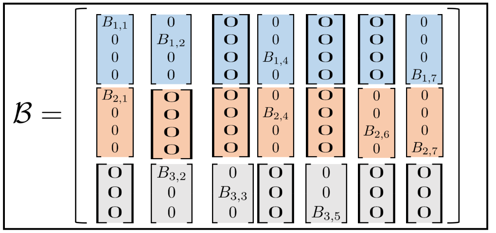
We also need to represent the term ∑e∈ℰkBe,k𝖳​vk,i−1e\sum_{e\in{\mathcal{E}}_{k}}B_{e,k}^{\mathsf{T}}v^{e}_{k,i-1} in terms of the network quantity 𝒴i−1{\scriptstyle{\mathcal{Y}}}_{i-1} defined in (24). To do that we first rewrite each term Be,k𝖳​vk,i−1eB_{e,k}^{\mathsf{T}}v^{e}_{k,i-1} in terms of the sub-network vector 𝒴i−1e{\scriptstyle{\mathcal{Y}}}_{i-1}^{e}. This can be simply done by introducing the 1×Ne1\times N_{e} block row matrix ℬe​k𝖳{\mathcal{B}}_{ek}^{\mathsf{T}} of similar block structure as 𝒴i−1e{\scriptstyle{\mathcal{Y}}}_{i-1}^{e} such that ℬe​k𝖳​𝒴i−1e=Be,k𝖳​yk,i−1e{\mathcal{B}}_{ek}^{\mathsf{T}}{\scriptstyle{\mathcal{Y}}}^{e}_{i-1}=B_{e,k}^{\mathsf{T}}y^{e}_{k,i-1} if k∈𝒞ek\in{\mathcal{C}}_{e} and zero otherwise – Figure 3 illustrates this construction. This construction can be represented by:

ℬe​k𝖳\displaystyle{\mathcal{B}}^{\mathsf{T}}_{ek} =blkrow​{Be,k​k′𝖳}k′∈𝒞e\displaystyle={\rm blkrow}\{B^{\mathsf{T}}_{e,kk^{\prime}}\}_{k^{\prime}\in{\mathcal{C}}_{e}} (30a)
Be,k​k′𝖳\displaystyle B^{\mathsf{T}}_{e,kk^{\prime}} =Δ{Be,k𝖳,ifk∈𝒞e,k=k′0Qk,Se,otherwise\displaystyle\;\stackrel{{\scriptstyle\Delta}}{{=}}\;\begin{cases}\begin{aligned} &B_{e,k}^{\mathsf{T}},&\ &\text{if}\ \ k\in{\mathcal{C}}_{e}\ ,k=k^{\prime}\\ &0_{Q_{k},S_{e}},&\ \ &\text{otherwise}\end{aligned}\end{cases} (30b)

Thus, we have ∑e∈ℰkBe,k𝖳​vk,i−1e=∑e=1Eℬe​k𝖳​𝒴i−1e\sum_{e\in{\mathcal{E}}_{k}}B_{e,k}^{\mathsf{T}}v^{e}_{k,i-1}=\sum_{e=1}^{E}{\mathcal{B}}_{ek}^{\mathsf{T}}{\scriptstyle{\mathcal{Y}}}^{e}_{i-1}.

Refer to caption
Fig. 3: An illustration of constructions (23) and (24) for the network in Figure 2 as well as construction (30) for agent k=4k=4 in that network.

If we let

ℬ\displaystyle{\mathcal{B}} =Δ[ℬ11⋯ℬ1​KℬE​1⋯ℬE​K]\displaystyle\;\stackrel{{\scriptstyle\Delta}}{{=}}\;\begin{bmatrix}{\mathcal{B}}_{11}&\cdots&{\mathcal{B}}_{1K}\\ \vdots&&\vdots\\ {\mathcal{B}}_{E1}&\cdots&{\mathcal{B}}_{EK}\end{bmatrix} (31)

then algorithm (22) can be rewritten compactly as follows:

𝒲i\displaystyle{\scriptstyle{\mathcal{W}}}_{i} =proxμw​ℛ(𝒲i−1−μw∇𝒥(𝒲i−1)−μwℬ𝖳𝒴i−1)\displaystyle=\scalebox{1}{\mbox{$\displaystyle\underset{\mu_{w}{\mathcal{R}}}{{\rm prox}}\big({\scriptstyle{\mathcal{W}}}_{i-1}-\mu_{w}{\nabla}{\mathcal{J}}({\scriptstyle{\mathcal{W}}}_{i-1})-\mu_{w}{\mathcal{B}}^{\mathsf{T}}{\scriptstyle{\mathcal{Y}}}_{i-1}\big)$}} (32a)
𝒴i\displaystyle{\scriptstyle{\mathcal{Y}}}_{i} =𝒜¯​(2​𝒴i−1−𝒴i−2+μv​ℬ​(𝒲i−𝒲i−1))\displaystyle=\bar{{\mathcal{A}}}\bigg(2{\scriptstyle{\mathcal{Y}}}_{i-1}-{\scriptstyle{\mathcal{Y}}}_{i-2}+\mu_{v}{\mathcal{B}}({\scriptstyle{\mathcal{W}}}_{i}-{\scriptstyle{\mathcal{W}}}_{i-1})\bigg) (32b)

for i≥1i\geq 1 with initialization:

𝒴0\displaystyle{\scriptstyle{\mathcal{Y}}}_{0} =𝒴−1+μv​(ℬ​𝒲0−b)\displaystyle={\scriptstyle{\mathcal{Y}}}_{-1}+\mu_{v}({\mathcal{B}}{\scriptstyle{\mathcal{W}}}_{0}-b) (33)

Notice that step (32b) depends on the two previous estimates; thus it is tedious to analyze directly. Therefore, to facilitate our analysis we will rewrite it in an equivalent form. To do that, we let:

𝒜=blkdiag​{Ae⊗ISe}e=1E\displaystyle{\mathcal{A}}={\rm blkdiag}\{A_{e}\otimes I_{S_{e}}\}_{e=1}^{E} (34)

and introduce the singular value (or eigenvalue for symmetric matrices) decomposition [43]:

0.5​(IN−𝒜)=[𝒰1𝒰2]​[Σ000]​[𝒰1𝖳𝒰2𝖳]=𝒰1​Σ​𝒰1𝖳\displaystyle 0.5(I_{N}-{\mathcal{A}})=\begin{bmatrix}{\mathcal{U}}_{1}&{\mathcal{U}}_{2}\end{bmatrix}\begin{bmatrix}\Sigma&0\\ 0&0\end{bmatrix}\begin{bmatrix}{\mathcal{U}}_{1}^{\mathsf{T}}\\ {\mathcal{U}}_{2}^{\mathsf{T}}\end{bmatrix}={\mathcal{U}}_{1}\Sigma{\mathcal{U}}_{1}^{\mathsf{T}} (35)

where N=∑e=1ENe​SeN=\sum_{e=1}^{E}N_{e}S_{e}, 𝒰1∈ℝN×r{\mathcal{U}}_{1}\in{\mathbb{R}}^{N\times r}, 𝒰2∈ℝN×(N−r){\mathcal{U}}_{2}\in{\mathbb{R}}^{N\times(N-r)}, and Σ=diag​{λj}j=1r\Sigma={\rm diag}\{\lambda_{j}\}_{j=1}^{r} with λr≤⋯≤λ1\lambda_{r}\leq\cdots\leq\lambda_{1} denoting the non-zero eigenvalues of the matrix 0.5​(I−𝒜)0.5(I-{\mathcal{A}}). Using an approach similar to the one used in [44], we can rewrite (32b) equivalently as follows — see Appendix A:

𝒳i\displaystyle{\scriptstyle{\scalebox{0.7}{\mbox{$\displaystyle\mathcal{X}$}}}}_{i}

=𝒳i−1−1μv​𝒰1𝖳​(𝒴i−1+μv​(ℬ​𝒲i−b)+μv​𝒰1​Σ​𝒳i−1)\displaystyle=\scalebox{0.95}{\mbox{$\displaystyle{\scriptstyle{\scalebox{0.7}{\mbox{$\displaystyle\mathcal{X}$}}}}_{i-1}-{1\over\mu_{v}}{\mathcal{U}}_{1}^{\mathsf{T}}\big({\scriptstyle{\mathcal{Y}}}_{i-1}+\mu_{v}({\mathcal{B}}{\scriptstyle{\mathcal{W}}}_{i}-b)+\mu_{v}{\mathcal{U}}_{1}\Sigma{\scriptstyle{\scalebox{0.7}{\mbox{$\displaystyle\mathcal{X}$}}}}_{i-1}\big)$}}\hskip-2.84526pt (36a)

𝒴i\displaystyle{\scriptstyle{\mathcal{Y}}}_{i}

=𝒴i−1+μv​(ℬ​𝒲i−b)+μv​𝒰1​Σ​𝒳i\displaystyle=\scalebox{0.95}{\mbox{$\displaystyle{\scriptstyle{\mathcal{Y}}}_{i-1}+\mu_{v}\big({\mathcal{B}}{\scriptstyle{\mathcal{W}}}_{i}-b\big)+\mu_{v}{\mathcal{U}}_{1}\Sigma{\scriptstyle{\scalebox{0.7}{\mbox{$\displaystyle\mathcal{X}$}}}}_{i}$}}\hskip-2.84526pt (36b)

for i≥1i\geq 1, where we introduced a new sequence 𝒳i{\scriptstyle{\scalebox{0.7}{\mbox{$\displaystyle\mathcal{X}$}}}}_{i} with 𝒳0=0{\scriptstyle{\scalebox{0.7}{\mbox{$\displaystyle\mathcal{X}$}}}}_{0}=0. Note that since AeA_{e} is primitive, symmetric, and doubly stochastic, it holds that the eigenvalues of the matrix AeA_{e} are in (−1,1](-1,1] – see [38, Lemma F.4]. Thus, from the block structure of 𝒜{\mathcal{A}} in (34), the eigenvalues of the matrix 0.5​(I−𝒜)0.5(I-{\mathcal{A}}) are in [0,1)[0,1). Therefore, the non-zero eigenvalues are positive and satisfy:

0<λr≤⋯≤λ1<1\displaystyle 0<\lambda_{r}\leq\cdots\leq\lambda_{1}<1 (37)

This property is useful for our convergence analysis.

V Convergence Results

In this section, we give the Lemmas leading to the main convergence results. The following auxiliary result is proven in [45].

Lemma 1.

For any N×NN\times N symmetric and doubly stochastic matrix AA, it holds that IN−AI_{N}-A is symmetric and positive semi-definite. If in addition AA is primitive and we let 𝒜=A⊗IM{\mathcal{A}}=A\otimes I_{M}, then, for any block vector 𝒵=col​{z1,…,zN}{\scriptstyle{\scalebox{0.85}{\mbox{$\displaystyle\mathcal{Z}$}}}}=\text{col}\{z^{1},...,z^{N}\} in the nullspace of I−𝒜I-{\mathcal{A}} with entries zn∈ℝMz^{n}\in\mathbb{R}^{M} it holds that:

(I−𝒜)​𝒵=0⇔z1=z2=…=zN\displaystyle(I-{\mathcal{A}}){\scriptstyle{\scalebox{0.85}{\mbox{$\displaystyle\mathcal{Z}$}}}}=0\iff z^{1}=z^{2}=...=z^{N} (38)

□\Box

Lemma 1 will be used in the proof of the next Lemma to show that consensus is reached at the optimality conditions.

Lemma 2.

(Optimality condition) If there exists a point (𝒲⋆,𝒴⋆,𝒳⋆)({\scriptstyle{\mathcal{W}}}^{\star},{\scriptstyle{\mathcal{Y}}}^{\star},{\scriptstyle{\scalebox{0.7}{\mbox{$\displaystyle\mathcal{X}$}}}}^{\star}) and a subgradient g⋆∈∂𝒲ℛ⁡(𝒲⋆)g^{\star}\in\partial_{{\scriptstyle{\scalebox{0.5}{\mbox{$\displaystyle\mathcal{W}$}}}}}{\mathcal{R}}({\scriptstyle{\mathcal{W}}}^{\star}) such that:

∇𝒥​(𝒲⋆)+g⋆+ℬ𝖳​𝒴⋆\displaystyle{\nabla}{\mathcal{J}}({\scriptstyle{\mathcal{W}}}^{\star})+g^{\star}+{\mathcal{B}}^{\mathsf{T}}{\scriptstyle{\mathcal{Y}}}^{\star} =0\displaystyle=0 (39a)
𝒰1𝖳​𝒴⋆\displaystyle{\mathcal{U}}_{1}^{\mathsf{T}}{\scriptstyle{\mathcal{Y}}}^{\star} =0\displaystyle=0 (39b)
(ℬ​𝒲⋆−b)+𝒰1​Σ​𝒳⋆\displaystyle({\mathcal{B}}{\scriptstyle{\mathcal{W}}}^{\star}-b)+{\mathcal{U}}_{1}\Sigma{\scriptstyle{\scalebox{0.7}{\mbox{$\displaystyle\mathcal{X}$}}}}^{\star} =0\displaystyle=0 (39c)

Then, it holds that vke,⋆=ve,⋆v^{e,\star}_{k}=v^{e,\star} ∀k∈𝒞e\forall\ k\in\mathcal{C}_{e} where (𝒲⋆,v1,⋆,⋯,ve,⋆)({\scriptstyle{\mathcal{W}}}^{\star},v^{1,\star},\cdots,v^{e,\star}) is a saddle point for the Lagrangian (10).

Proof: A similar argument appears in the conference version [1, Lemma 2] except for the addition of sub-gradient terms into the argument. Using the block structure of ∇𝒥(.){\nabla}{\mathcal{J}}(.) and ℬ{\mathcal{B}} in (29) and (30)–(31), we can expand (39a) into its components to get:

∇wkJk​(wk⋆)+gk⋆+∑e∈ℰkBe,k𝖳​vke,⋆=0,∀k\displaystyle{\nabla}_{w_{k}}J_{k}(w_{k}^{\star})+g_{k}^{\star}+\sum_{e\in{\mathcal{E}}_{k}}B_{e,k}^{\mathsf{T}}v_{k}^{e,\star}=0,\quad\forall\ k (40)

where gk⋆∈∂wkRk​(wk⋆)g_{k}^{\star}\in\partial_{w_{k}}R_{k}(w_{k}^{\star}). From the fact 𝒰1𝖳​𝒰1=I{\mathcal{U}}_{1}^{\mathsf{T}}{\mathcal{U}}_{1}=I and Σ>0\Sigma>0, condition (39b) is equivalent to:

𝒰1𝖳​𝒴⋆=0⇔𝒰1​Σ​𝒰1𝖳​𝒴⋆=0⇔12​(I−𝒜)​𝒴⋆=0\displaystyle{\mathcal{U}}_{1}^{\mathsf{T}}{\scriptstyle{\mathcal{Y}}}^{\star}=0\iff{\mathcal{U}}_{1}\Sigma{\mathcal{U}}_{1}^{\mathsf{T}}{\scriptstyle{\mathcal{Y}}}^{\star}=0\iff{1\over 2}(I-{\mathcal{A}}){\scriptstyle{\mathcal{Y}}}^{\star}=0

(41)

Therefore, from (38), and the block structure of 𝒜{\mathcal{A}} in (34), condition (39b) gives:

vke,⋆=vse,⋆=ve,⋆,∀k,s∈𝒞e\displaystyle v^{e,\star}_{k}=v^{e,\star}_{s}=v^{e,\star},\quad\forall\ k,s\in{\mathcal{C}}_{e} (42)

for some ve,⋆v^{e,\star}. Hence, condition (40) satisfies the first optimality condition for problem (5) – see [37]. Now, let 𝒵=blkdiag​{𝟙Ne⊗ISe}e=1E{\mathcal{Z}}={\rm blkdiag}\{\mathds{1}_{N_{e}}\otimes I_{S_{e}}\}_{e=1}^{E}. Multiplying equation (39c) on the left by 𝒵𝖳{\mathcal{Z}}^{\mathsf{T}} gives:

0=𝒵𝖳​(ℬ​𝒲⋆−b)+𝒵𝖳​𝒰1⏟=0​Σ​𝒳⋆​=(a)​𝒵𝖳​(ℬ​𝒲⋆−b)\displaystyle 0={\mathcal{Z}}^{\mathsf{T}}({\mathcal{B}}{\scriptstyle{\mathcal{W}}}^{\star}-b)+\underbrace{{\mathcal{Z}}^{\mathsf{T}}{\mathcal{U}}_{1}}_{=0}\Sigma{\scriptstyle{\scalebox{0.7}{\mbox{$\displaystyle\mathcal{X}$}}}}^{\star}\overset{(a)}{=}{\mathcal{Z}}^{\mathsf{T}}({\mathcal{B}}{\scriptstyle{\mathcal{W}}}^{\star}-b) (43)

where step (a) holds because because from (38), 𝒵{\mathcal{Z}} is in the nullspace of I−𝒜I-{\mathcal{A}} and thus also in the nullspace of 𝒰1𝖳{\mathcal{U}}_{1}^{\mathsf{T}} [1, Equation (51)]. Using the block structure of ℬ{\mathcal{B}} and bb in (30)–(31) and (25), we can also expand (43) into its components to get:

(𝟙Ne𝖳⊗ISe)​(∑k=1K(ℬe​k​wk⋆)−be)\displaystyle(\mathds{1}_{N_{e}}^{\mathsf{T}}\otimes I_{S_{e}})\bigg(\sum_{k=1}^{K}({\mathcal{B}}_{ek}w_{k}^{\star})-b_{e}\bigg) =∑k∈𝒞e(Be,k​wk⋆−be,k)\displaystyle=\sum_{k\in{\mathcal{C}}_{e}}\left(B_{e,k}w_{k}^{\star}-b_{e,k}\right)
=0\displaystyle=0 (44)

for all ee since

ℬe​k𝖳​(𝟙Ne⊗ISe)\displaystyle{\mathcal{B}}_{ek}^{\mathsf{T}}(\mathds{1}_{N_{e}}\otimes I_{S_{e}})

=∑k′∈𝒞eBe,k​k′𝖳={Be,k𝖳,if ​k∈𝒞e0,otherwise\displaystyle=\scalebox{0.975}{\mbox{$\displaystyle\sum_{k^{\prime}\in{\mathcal{C}}_{e}}B_{e,kk^{\prime}}^{\mathsf{T}}=\begin{cases}\begin{aligned} &B_{e,k}^{\mathsf{T}},\ &\text{if }k\in{\mathcal{C}}_{e}\\ &0,&\text{otherwise}\end{aligned}\end{cases}$}} (45)

Equation (44) is the second optimality condition for problem (5) and, thus, (𝒲⋆,v1,⋆,⋯,ve,⋆)({\scriptstyle{\mathcal{W}}}^{\star},v^{1,\star},\cdots,v^{e,\star}) is an optimal point for (14) [37]. □\Box

Remark 2 (Existence and uniqueness).

Note that there exists a point (𝒲⋆,𝒴⋆,𝒳⋆)({\scriptstyle{\mathcal{W}}}^{\star},{\scriptstyle{\mathcal{Y}}}^{\star},{\scriptstyle{\scalebox{0.7}{\mbox{$\displaystyle\mathcal{X}$}}}}^{\star}) that satisfies the optimality conditions (39). Specifically, if 𝒲⋆=col⁡{wk⋆}{\scriptstyle{\mathcal{W}}}^{\star}={\rm col}\{w_{k}^{\star}\} and 𝒴⋆=col​{𝟙Ne⊗ve,⋆}e=1E{\scriptstyle{\mathcal{Y}}}^{\star}={\rm col}\{\mathds{1}_{N_{e}}\otimes v^{e,\star}\}_{e=1}^{E}, where (𝒲⋆,v1,⋆,⋯,vE,⋆)({\scriptstyle{\mathcal{W}}}^{\star},v^{1,\star},\cdots,v^{E,\star}) is an optimal solution of the saddle point problem (14), then, it can be easily verified that conditions (39a)–(39b) are satisfied. Now, by following an argument similar to the one used in [46, Lemma  3], it can be shown that there exists an 𝒳⋆{\scriptstyle{\scalebox{0.7}{\mbox{$\displaystyle\mathcal{X}$}}}}^{\star} such that (39c) holds; moreover, there exists a unique 𝒳⋆{\scriptstyle{\scalebox{0.7}{\mbox{$\displaystyle\mathcal{X}$}}}}^{\star} in the range space of 𝒰1𝖳{\mathcal{U}}_{1}^{\mathsf{T}}. Now, we know from strong convexity that 𝒲⋆{\scriptstyle{\mathcal{W}}}^{\star} is unique. Thus, from (39a), the dual point 𝒴⋆{\scriptstyle{\mathcal{Y}}}^{\star} is unique if the matrix ℬ{\mathcal{B}} has full row rank. Under this condition and in the absence of non-smooth terms, we will show that our algorithm converges linearly to this unique point – see Theorem 2 . □\Box

Remark 3.

The analysis technique used in this work is not related to the techniques used in [46, 30]. Note that this work deals with a non-smooth saddle-point problem where the dual variables are shared across agents, while the works [46, 30] deal with smooth minimization problems with a shared primal variable and twice-differentiable functions. □\Box

We will now show that the equivalent network recursions (32a) and (36a)–(36b) of the proposed algorithm converge to a point that satisfies the optimality conditions given in Lemma 2. To give the convergence results, we introduce the error vectors:

𝒲~i=Δ𝒲⋆−𝒲i,𝒳~i=Δ𝒳⋆−𝒳i𝒴~i\displaystyle\widetilde{\scriptstyle{\mathcal{W}}}_{i}\;\stackrel{{\scriptstyle\Delta}}{{=}}\;{\scriptstyle{\mathcal{W}}}^{\star}-{\scriptstyle{\mathcal{W}}}_{i},\quad\widetilde{\scriptstyle{\mathcal{X}}}_{i}\;\stackrel{{\scriptstyle\Delta}}{{=}}\;{\scriptstyle{\scalebox{0.7}{\mbox{$\displaystyle\mathcal{X}$}}}}^{\star}-{\scriptstyle{\scalebox{0.7}{\mbox{$\displaystyle\mathcal{X}$}}}}_{i}\quad\widetilde{\scriptstyle{\mathcal{Y}}}_{i} =Δ𝒴⋆−𝒴i\displaystyle\;\stackrel{{\scriptstyle\Delta}}{{=}}\;{\scriptstyle{\mathcal{Y}}}^{\star}-{\scriptstyle{\mathcal{Y}}}_{i} (46)

and the diagonal matrix:

𝒟=Δμv​(Σ−Σ2)>0\displaystyle{\mathcal{D}}\;\stackrel{{\scriptstyle\Delta}}{{=}}\;\mu_{v}(\Sigma-\Sigma^{2})>0 (47)

where Σ\Sigma was introduced in (35). Note that 𝒟{\mathcal{D}} is positive definite because of (37).

Lemma 3.

(Primal-dual bound): Suppose Assumptions 1-3 hold, then:

‖𝒲~i‖2−‖𝒲~i−1‖2\displaystyle\|\widetilde{\scriptstyle{\mathcal{W}}}_{i}\|^{2}-\|\widetilde{\scriptstyle{\mathcal{W}}}_{i-1}\|^{2} ≤−(1−μw​(2​δ−ν))​‖𝒲i−𝒲i−1‖2\displaystyle\leq-\big(1-\mu_{w}(2\delta-\nu)\big)\|{\scriptstyle{\mathcal{W}}}_{i}-{\scriptstyle{\mathcal{W}}}_{i-1}\|^{2}
−μw​ν​(‖𝒲~i−1‖2+‖𝒲~i‖2)\displaystyle\quad-\mu_{w}\nu\left(\|\widetilde{\scriptstyle{\mathcal{W}}}_{i-1}\|^{2}+\|\widetilde{\scriptstyle{\mathcal{W}}}_{i}\|^{2}\right)
−2​μw​(𝒴i−1−𝒴⋆)𝖳​ℬ​(𝒲i−𝒲⋆)\displaystyle\quad-2\mu_{w}({\scriptstyle{\mathcal{Y}}}_{i-1}-{\scriptstyle{\mathcal{Y}}}^{\star})^{\mathsf{T}}{\mathcal{B}}({\scriptstyle{\mathcal{W}}}_{i}-{\scriptstyle{\mathcal{W}}}^{\star}) (48)

and

‖𝒴~i‖μv−12+‖𝒳~i‖𝒟2−‖𝒴~i−1‖μv−12−‖𝒳~i−1‖𝒟2\displaystyle\|\widetilde{\scriptstyle{\mathcal{Y}}}_{i}\|^{2}_{\mu_{v}^{-1}}+\|\widetilde{\scriptstyle{\mathcal{X}}}_{i}\|_{\mathcal{D}}^{2}-\|\widetilde{\scriptstyle{\mathcal{Y}}}_{i-1}\|_{\mu_{v}^{-1}}^{2}-\|\widetilde{\scriptstyle{\mathcal{X}}}_{i-1}\|_{\mathcal{D}}^{2}
=−‖𝒳i−𝒳i−1‖𝒟2−‖Σ​𝒳~i‖μv2+‖ℬ​𝒲~i‖μv2\displaystyle=-\|{\scriptstyle{\scalebox{0.7}{\mbox{$\displaystyle\mathcal{X}$}}}}_{i}-{\scriptstyle{\scalebox{0.7}{\mbox{$\displaystyle\mathcal{X}$}}}}_{i-1}\|_{\mathcal{D}}^{2}-\|\Sigma\widetilde{\scriptstyle{\mathcal{X}}}_{i}\|_{\mu_{v}}^{2}+\|{\mathcal{B}}\widetilde{\scriptstyle{\mathcal{W}}}_{i}\|_{\mu_{v}}^{2}
+2​(𝒴i−1−𝒴⋆)𝖳​ℬ​(𝒲i−𝒲⋆)\displaystyle\quad+2({\scriptstyle{\mathcal{Y}}}_{i-1}-{\scriptstyle{\mathcal{Y}}}^{\star})^{\mathsf{T}}{\mathcal{B}}({\scriptstyle{\mathcal{W}}}_{i}-{\scriptstyle{\mathcal{W}}}^{\star}) (49)

where (𝒲⋆,𝒴⋆,𝒳⋆)({\scriptstyle{\mathcal{W}}}^{\star},{\scriptstyle{\mathcal{Y}}}^{\star},{\scriptstyle{\scalebox{0.7}{\mbox{$\displaystyle\mathcal{X}$}}}}^{\star}) satisfy the optimality conditions given in Lemma 2.

Proof: See Appendices B and C. □\Box

The previous Lemma is used to establish the following theorem.

Theorem 1.

(Convergence): Suppose Assumptions 1–3 hold, then for positive constant step-sizes satisfying:

μw<12​δ−ν,μv<νλmax​(ℬ𝖳​ℬ)\displaystyle\mu_{w}<{1\over 2\delta-\nu},\quad\mu_{v}<{\nu\over\lambda_{\max}({\mathcal{B}}^{\mathsf{T}}{\mathcal{B}})} (50)

recursions (32a) and (36a)–(36b) converge and it holds that 𝒲i{\scriptstyle{\mathcal{W}}}_{i} converges to the optimal solution of (5).

Proof: See Appendix D. □\Box

At this point we showed that the dual coupled diffusion strategy, which handles non-smooth terms, converges to the optimal point. However, it is still unclear how the sparsity of the constraints affects the convergence behavior. Apart from saving communication and memory, the next result reveals the advantage of exploiting the constraint structure.

Theorem 2.

(Linear convergence): Suppose Assumptions 1–3 hold, and, furthermore, assume that each Rk​(wk)=0R_{k}(w_{k})=0 and each matrix blkcol​{Be,k}e∈ℰk{\rm blkcol}\{B_{e,k}\}_{e\in{\mathcal{E}}_{k}} has full row rank. If the step sizes satisfy (50), then it holds that:

‖𝒲~i‖Cw2+‖𝒴~i‖μwμv2+‖𝒳~i‖μw​μv​Σ2≤γi​C0\displaystyle\|\widetilde{\scriptstyle{\mathcal{W}}}_{i}\|_{C_{w}}^{2}+\|\widetilde{\scriptstyle{\mathcal{Y}}}_{i}\|^{2}_{\mu_{w}\over\mu_{v}}+\|\widetilde{\scriptstyle{\mathcal{X}}}_{i}\|_{\mu_{w}\mu_{v}\Sigma}^{2}\leq\gamma^{i}C_{0} (51)

for some constant C0>0C_{0}>0 where Cw=I−μw​μv​ℬ𝖳​ℬ>0C_{w}=I-\mu_{w}\mu_{v}{\mathcal{B}}^{\mathsf{T}}{\mathcal{B}}>0 and

γ=Δmax⁡{γ1,γ2,1−λr}<1\displaystyle\gamma\;\stackrel{{\scriptstyle\Delta}}{{=}}\;\max\big\{\gamma_{1},\gamma_{2},1-\lambda_{r}\big\}<1 (52)

with γ1=1−μw​ν​(1−δ​μw)\gamma_{1}=1-\mu_{w}\nu(1-\delta\mu_{w}), γ2=1−μw​μv​λmin​(ℬ​ℬ𝖳)\gamma_{2}=1-\mu_{w}\mu_{v}\lambda_{\min}({\mathcal{B}}{\mathcal{B}}^{\mathsf{T}}) and λr\lambda_{r} denoting the smallest non-zero eigenvalue of 0.5​(I−𝒜)0.5(I-{\mathcal{A}}).

Proof: See Appendix E. □\Box

The above result shows why solving (5) directly is important for at least two reasons. First, by using model (5), we are able to prove linear convergence under the assumption that each blkcol​{Be,k}e∈ℰk{\rm blkcol}\{B_{e,k}\}_{e\in{\mathcal{E}}_{k}} has full row rank. If instead, we were to rewrite problem (5) into the form (1) by embedding zeros into the matrices BkB_{k}, then our analysis would require BkB_{k} to be full row rank for linear convergence. This will not be satisfied if some agent is not involved in some constraint since in that case BkB_{k} will have zero rows and, thus, BkB_{k} is row rank deficient even if blkcol​{Be,k}e∈ℰk{\rm blkcol}\{B_{e,k}\}_{e\in{\mathcal{E}}_{k}} has full row rank.

The second more important reason is that the convergence rate depends on the connectivity of the sub-networks 𝒞e{\mathcal{C}}_{e} and not on the connectivity of the entire network, as we illustrate now. Note from the block structure of (34) that the smallest non-negative eigenvalue of 0.5​(I−𝒜)0.5(I-{\mathcal{A}}) has the form λr=mine⁡σ¯e\lambda_{r}=\min_{e}\underline{\sigma}_{e} where σ¯e\underline{\sigma}_{e} denotes the smallest non-zero eigenvalue of the matrix 0.5​(I−Ae)0.5(I-A_{e}). Since I−0.5​(I−Ae)=0.5​(I+Ae)=Ae¯I-0.5(I-A_{e})=0.5(I+A_{e})=\bar{A_{e}}, it holds that 1−σ¯e=λ¯2,e1-\underline{\sigma}_{e}=\bar{\lambda}_{2,e}, where λ¯2,e\bar{\lambda}_{2,e} denotes the second largest eigenvalue of A¯e\bar{A}_{e} (the largest eigenvalue is equal to one). Therefore,

1−λr=1−mine⁡σ¯e=maxe⁡(1−σ¯e)=maxe⁡λ¯2,e\displaystyle 1-\lambda_{r}=1-\min_{e}\underline{\sigma}_{e}=\max_{e}(1-\underline{\sigma}_{e})=\max_{e}\bar{\lambda}_{2,e} (53)

Thus, assuming 1−λr1-\lambda_{r} is dominating the convergence rate, then the smaller maxe⁡λ¯2,e\max_{e}\bar{\lambda}_{2,e} is, the faster the algorithm is. We see that this depends on the second largest eigenvalue of the matrices {A¯e}\{\bar{A}_{e}\}, which depends on the sub-networks connectivity and not the whole network. This observation reveals the importance of the algorithm for sparse networks and under sparsely coupled constraints. Since in that case the small sub-networks are much well connected than the whole network. This observation will be illustrated in the simulation section next.

Remark 4 (Condition Number).

By using the the upper bound (50), we conclude from Theorem 2 that the number of iterations needed to reach ϵ\epsilon accuracy is on the order of

O⁡(max⁡{κJ​κB,1/λr}​log​1ϵ)\displaystyle O\left(\max\{\kappa_{J}\kappa_{B},1/\lambda_{r}\}{\rm log}{1\over\epsilon}\right)

where κJ=δ/ν\kappa_{J}=\delta/\nu and κB=λmax​(ℬ​ℬ𝖳)/λmin​(ℬ​ℬ𝖳)\kappa_{B}=\lambda_{\max}({\mathcal{B}}{\mathcal{B}}^{\mathsf{T}})/\lambda_{\min}({\mathcal{B}}{\mathcal{B}}^{\mathsf{T}}) are the condition numbers of the cost 𝒥(.){\mathcal{J}}(.) and the matrix ℬ​ℬ𝖳{\mathcal{B}}{\mathcal{B}}^{\mathsf{T}}, respectively. □\Box

Refer to caption
(a) Network topology used in simulations.
(b) Least squares results.
(c) Logistic regression results.
Fig. 4: Simulation results. *Dual diffusion refers to (22) applied on the same problem reformulated into (1), which ignores the sparsity structure. Similarly, both IDC-ADMM [15] and ”dual DIGing” [47] are designed for problem (1) and ignore the sparsity structure.

VI Numerical Simulation

In this section, we test the performance of the proposed algorithm with two numerical experiments.

  • •

    Distributed Linear Regression: The first set-up considers a linear regression problem with costs:

    Jk​(wk)=12​Tk​∑t=1Tk‖uk,t𝖳​wk−pk​(t)‖2\displaystyle J_{k}(w_{k})=\frac{1}{2T_{k}}\sum_{t=1}^{T_{k}}\|u_{k,t}^{\mathsf{T}}w_{k}-p_{k}(t)\|^{2}

    and Rk​(wk)=η1​‖wk‖1R_{k}(w_{k})=\eta_{1}\|w_{k}\|_{1} where uk,t∈ℝQku_{k,t}\in{\mathbb{R}}^{Q_{k}} is the regressor vector for data sample tt, pk​(t)∈ℝp_{k}(t)\in{\mathbb{R}}, and TkT_{k} denotes the amount of data for agent kk.

  • •

    Distributed Logistic Regression: The second set-up considers a logistic regression problem with costs:

    Jk​(wk)=1Tk​∑t=1Tkln⁡(1+exp⁡(−xk​(t)​hk,t𝖳​wk))+0.5​η2​‖wk‖2\displaystyle J_{k}(w_{k})=\frac{1}{T_{k}}\sum_{t=1}^{T_{k}}\ln\left(1+\exp(-x_{k}(t)h_{k,t}^{\mathsf{T}}w_{k})\right)+0.5\eta_{2}\|w_{k}\|^{2}

    and Rk​(wk)=η1​‖wk‖1R_{k}(w_{k})=\eta_{1}\|w_{k}\|_{1}. The vector hk,t∈ℝQkh_{k,t}\in{\mathbb{R}}^{Q_{k}} is the regressor vector for data sample tt, and xk​(t)x_{k}(t) is the label for that data sample, which is either +1+1 or −1-1.

In both experiments, the network used is shown in Fig. 4(a) with K=20K=20 agents. The positions (xx-axis and yy-axis) of the agents are randomly generated in ([0,1],[0,1])([0,1],[0,1]), and two agents are connected if the distance between them is less than or equal d=0.3d=0.3. As for the constraints, we assume E=K=20E=K=20, and each constraint ee (or kk) (where e∈{1,⋯,20}e\in\{1,\cdots,20\}) is associated with a subnetwork involving agent ee (or kk) and all its neighbors as described in equation (2). Each element in Be,kB_{e,k} is generated according to the standard Gaussian distribution 𝒩⁡(0,1){\mathcal{N}}(0,1). Each be,kb_{e,k} is also randomly generated and we guarantee that there exists a feasible solution to (5). All the combination matrices are generated according to the Metropolis rule.

In the first simulation, we set Tk=1000T_{k}=1000 for all kk and each regressor uk,tu_{k,t} is generated according to the Gaussian distribution 𝒩⁡(0,1){\mathcal{N}}(0,1). To generate the associated pk​(t)p_{k}(t), we first generate a vector wk,0∈ℝQkw_{k,0}\in{\mathbb{R}}^{Q_{k}} randomly from 𝒩⁡(0,1){\mathcal{N}}(0,1). We let 20%20\% of the entries of w0,kw_{0,k} to be 00. With such sparse wk,0w_{k,0}, we generate pk​(t)p_{k}(t) as pk​(t)=uk,t𝖳​wk,0+nkp_{k}(t)=u_{k,t}^{\mathsf{T}}w_{k,0}+n_{k} where nk∼𝒩⁡(0,0.1)n_{k}\sim{\mathcal{N}}(0,0.1) is some Gaussian noise. In this experiment, we set Qk=10Q_{k}=10 for k=1,⋯,Kk=1,\cdots,K. We also set η1=0.3\eta_{1}=0.3 and Be,k∈ℝ3×10B_{e,k}\in{\mathbb{R}}^{3\times 10} to be an under-determined coefficient matrix. In the second set-up, each Tk=1000T_{k}=1000. Among all local data samples, half of them are generated by the Gaussian distribution 𝒩⁡(1,1){\mathcal{N}}(1,1) and their corresponding labels {xk​(t)}\{x_{k}(t)\} are +1+1’s. The other half are generated by 𝒩⁡(−1,1){\mathcal{N}}(-1,1) and their corresponding labels {xk​(t)}\{x_{k}(t)\} are −1-1’s. We set Qk=10Q_{k}=10 for k=1,⋯,Kk=1,\cdots,K and η1=η2=0.1\eta_{1}=\eta_{2}=0.1. We let Be,k∈ℝ3×10B_{e,k}\in{\mathbb{R}}^{3\times 10} to be an under-determined coefficient matrix.

Refer to caption
Fig. 5: A comparison of algorithm (22) for different network connectivity and under two implementations: dual coupled diffusion exploits structure while dual diffusion ignores the structure.

To illustrate the effect of the constraint structure, we consider two approaches to solve problem (5). The first approach is to use the dual coupled diffusion (22) while considering the structure of the problem (5), i.e., run (22) with E=K,𝒞e=𝒩eE=K,{\mathcal{C}}_{e}={\mathcal{N}}_{e}. The second approach is to ignore the special structure of the problem and reformulate it into the form of problem (1) and also run the dual coupled diffusion (22) with E=1,𝒞1={1,⋯,K}E=1,{\mathcal{C}}_{1}=\{1,\cdots,K\}, which we call dual diffusion. To compare with other related methods that only share dual variables, we simulate the inexact distributed consensus ADMM (IDC-ADMM) from [15] and a modified proximal version of the one in [47] in which the dual iterates are updated similar to the DIGing algorithm in [42], which we call “Dual DIGing”. Both of these algorithm are designed for problem (1) and ignores any structure. The step-sizes are chosen manually to get the best possible performance for each algorithm. In the first linear regression setup, the parameters used are (μw=0.28,μv=0.28)(\mu_{w}=0.28,\ \mu_{v}=0.28) for the dual coupled diffusion, (μw=0.28,μv=0.28)(\mu_{w}=0.28,\ \mu_{v}=0.28) for the dual diffusion, (c=0.25,μw=0.05)(c=0.25,\ \mu_{w}=0.05) for the IDC-ADMM [15], and the step-sizes are set to 0.450.45 for the dual DIGing method. In the second logistic regression set-up, they are set to (μw=0.2,μv=0.2)(\mu_{w}=0.2,\ \mu_{v}=0.2) for the dual coupled diffusion, (μw=0.2,μv=0.2)(\mu_{w}=0.2,\ \mu_{v}=0.2) for the dual diffusion, (c=0.45,μw=0.2)(c=0.45,\ \mu_{w}=0.2) for the IDC-ADMM [15], and the step-sizes are set to 0.180.18 for the dual DIGing method. Figure 4 shows the relative error 1K​∑k=1K‖wk,i−wk⋆‖2/‖wk⋆‖2\frac{1}{K}\sum_{k=1}^{K}\|w_{k,i}-w_{k}^{\star}\|^{2}/\|w_{k}^{\star}\|^{2} for each of the previous algorithms for both set-ups. Note that the dual DIGing algorithm requires communicating two vectors each round of communication. It is observed that dual diffusion, the IDC-ADMM, and the dual DIGing algorithms have a close performance (all ignores any structure), while the dual coupled diffusion clearly outperforms them. This means that, apart from requiring less amount of data to be exchanged per round of communication, our algorithm is also able to reach an ϵ\epsilon accuracy (where ϵ\epsilon is arbitrarily small) with much less time compared to these other algorithms. As explained before, this superiority is due to the sub-networks being better connected compared to the whole network and the dual coupled diffusion takes advantage of that. In this simulation, we have 1−λr=0.9111-\lambda_{r}=0.911 for the dual coupled diffusion and 1−λ=0.9731-\lambda=0.973 for the dual diffusion (we dropped the sub-index since we have one network combination matrix in this case), which backs up our theoretical findings.

To further illustrate the effect of the sub-networks connectivity on the convergence rate, we simulate the dual coupled diffusion (exploits sparsity) and dual diffusion (which does not exploit the sparsity) with the same logistic regression set-up from before but for the three different networks shown in top half of Fig. 5. The step sizes used in this simulation are adjusted to get the best possible results, which are shown on the bottom of Figure 5. Note that the network on the left has less connections compared to the network on the right, and thus, the sub-networks on the left are more sparse than the one on the right. Note further that for the constraints settings used (2), the more connections the network has, the closer the sub-networks are to the entire network. It is seen that dual coupled diffusion performs significantly better under sparser networks since in that case the sub-networks are much better connected than the whole network. On the other hand, when we add more connections, the sub-networks connectivity becomes closer to the network connectivity and, thus, the performance of the two algorithms become closer and closer. The performance will become identical when all agents are involved in all the constraint.

VII Concluding remarks

This work developed a proximal diffusion strategy with guaranteed exact convergence for a multi-agent optimization problem with multiple coupled constraints. We established analytically, and by means of simulations, the superior convergence properties of an algorithm that considers the sparsity structure in the constraints compared to others that ignore this structure.

Appendix A Equivalent Representation

In this appendix, we show that (36a)–(36b) is equivalent to (32b). Multiplying equation (36a) by 𝒰1​Σ{\mathcal{U}}_{1}\Sigma and then collecting the term 𝒰1​Σ​𝒳i−1{\mathcal{U}}_{1}\Sigma{\scriptstyle{\scalebox{0.7}{\mbox{$\displaystyle\mathcal{X}$}}}}_{i-1} we get:

𝒰1​Σ​𝒳i\displaystyle{\mathcal{U}}_{1}\Sigma{\scriptstyle{\scalebox{0.7}{\mbox{$\displaystyle\mathcal{X}$}}}}_{i} =(I−𝒰1​Σ​𝒰1𝖳)​𝒰1​Σ​𝒳i−1\displaystyle=(I-{\mathcal{U}}_{1}\Sigma{\mathcal{U}}_{1}^{\mathsf{T}}){\mathcal{U}}_{1}\Sigma{\scriptstyle{\scalebox{0.7}{\mbox{$\displaystyle\mathcal{X}$}}}}_{i-1}
−μv−1​(𝒰1​Σ​𝒰1𝖳)​(𝒴i−1+μv​(ℬ​𝒲i−b))\displaystyle\quad-\mu_{v}^{-1}\left({\mathcal{U}}_{1}\Sigma{\mathcal{U}}_{1}^{\mathsf{T}}\right)\bigg({\scriptstyle{\mathcal{Y}}}_{i-1}+\mu_{v}\big({\mathcal{B}}{\scriptstyle{\mathcal{W}}}_{i}-b\big)\bigg) (54)

Let 𝒳¯i=Δ𝒰1​Σ​𝒳i\bar{{\scriptstyle{\scalebox{0.7}{\mbox{$\displaystyle\mathcal{X}$}}}}}_{i}\;\stackrel{{\scriptstyle\Delta}}{{=}}\;{\mathcal{U}}_{1}\Sigma{\scriptstyle{\scalebox{0.7}{\mbox{$\displaystyle\mathcal{X}$}}}}_{i}. Using (35) and collecting the term 𝒳i−1{\scriptstyle{\scalebox{0.7}{\mbox{$\displaystyle\mathcal{X}$}}}}_{i-1} on the right hand side of the last equation, we get:

𝒳¯i\displaystyle\bar{{\scriptstyle{\scalebox{0.7}{\mbox{$\displaystyle\mathcal{X}$}}}}}_{i} =𝒜¯​𝒳¯i−1−μv−1​12​(I−𝒜)​(𝒴i−1+μv​(ℬ​𝒲i−b))\displaystyle=\bar{{\mathcal{A}}}\bar{{\scriptstyle{\scalebox{0.7}{\mbox{$\displaystyle\mathcal{X}$}}}}}_{i-1}-\mu_{v}^{-1}\frac{1}{2}\left(I-{\mathcal{A}}\right)\left({\scriptstyle{\mathcal{Y}}}_{i-1}+\mu_{v}\big({\mathcal{B}}{\scriptstyle{\mathcal{W}}}_{i}-b\big)\right) (55)

Multiplying (36b) by 𝒜¯\bar{{\mathcal{A}}} on the left and using the definition 𝒳¯i=Δ𝒰1​Σ​𝒳i\bar{{\scriptstyle{\scalebox{0.7}{\mbox{$\displaystyle\mathcal{X}$}}}}}_{i}\;\stackrel{{\scriptstyle\Delta}}{{=}}\;{\mathcal{U}}_{1}\Sigma{\scriptstyle{\scalebox{0.7}{\mbox{$\displaystyle\mathcal{X}$}}}}_{i} we have:

𝒜¯​𝒴i−1\displaystyle\bar{{\mathcal{A}}}{\scriptstyle{\mathcal{Y}}}_{i-1} =𝒜¯​𝒴i−2+μv​𝒜¯​(ℬ​𝒲i−1−b)+μv​𝒜¯​𝒳¯i−1\displaystyle=\bar{{\mathcal{A}}}{\scriptstyle{\mathcal{Y}}}_{i-2}+\mu_{v}\bar{{\mathcal{A}}}\big({\mathcal{B}}{\scriptstyle{\mathcal{W}}}_{i-1}-b\big)+\mu_{v}\bar{{\mathcal{A}}}\bar{{\scriptstyle{\scalebox{0.7}{\mbox{$\displaystyle\mathcal{X}$}}}}}_{i-1} (56)

Now, subtracting (56) from (36b) we get:

𝒴i−𝒜¯​𝒴i−1\displaystyle{\scriptstyle{\mathcal{Y}}}_{i}-\bar{{\mathcal{A}}}{\scriptstyle{\mathcal{Y}}}_{i-1}
=𝒴i−1−𝒜¯​𝒴i−2+μv​(ℬ​𝒲i−b)−μv​𝒜¯​(ℬ​𝒲i−1−b)\displaystyle={\scriptstyle{\mathcal{Y}}}_{i-1}-\bar{{\mathcal{A}}}{\scriptstyle{\mathcal{Y}}}_{i-2}+\mu_{v}\big({\mathcal{B}}{\scriptstyle{\mathcal{W}}}_{i}-b\big)-\mu_{v}\bar{{\mathcal{A}}}\big({\mathcal{B}}{\scriptstyle{\mathcal{W}}}_{i-1}-b\big)
+μv​(𝒳¯i−𝒜¯​𝒳¯i−1)\displaystyle\ +\mu_{v}(\bar{{\scriptstyle{\scalebox{0.7}{\mbox{$\displaystyle\mathcal{X}$}}}}}_{i}-\bar{{\mathcal{A}}}\bar{{\scriptstyle{\scalebox{0.7}{\mbox{$\displaystyle\mathcal{X}$}}}}}_{i-1}) (57)

Using (55) we can remove the term μv​(𝒳¯i−𝒜¯​𝒳¯i−1)\mu_{v}(\bar{{\scriptstyle{\scalebox{0.7}{\mbox{$\displaystyle\mathcal{X}$}}}}}_{i}-\bar{{\mathcal{A}}}\bar{{\scriptstyle{\scalebox{0.7}{\mbox{$\displaystyle\mathcal{X}$}}}}}_{i-1}) from the previous expression to get:

𝒴i−𝒜¯​𝒴i−1\displaystyle{\scriptstyle{\mathcal{Y}}}_{i}-\bar{{\mathcal{A}}}{\scriptstyle{\mathcal{Y}}}_{i-1}
=𝒴i−1−𝒜¯​𝒴i−2+μv​(ℬ​𝒲i−b)−μv​𝒜¯​(ℬ​𝒲i−1−b)\displaystyle={\scriptstyle{\mathcal{Y}}}_{i-1}-\bar{{\mathcal{A}}}{\scriptstyle{\mathcal{Y}}}_{i-2}+\mu_{v}\big({\mathcal{B}}{\scriptstyle{\mathcal{W}}}_{i}-b\big)-\mu_{v}\bar{{\mathcal{A}}}\big({\mathcal{B}}{\scriptstyle{\mathcal{W}}}_{i-1}-b\big)
−12​(I−𝒜)​(𝒴i−1+μv​(ℬ​𝒲i−b))\displaystyle\quad-\frac{1}{2}\left(I-{\mathcal{A}}\right)\left({\scriptstyle{\mathcal{Y}}}_{i-1}+\mu_{v}\big({\mathcal{B}}{\scriptstyle{\mathcal{W}}}_{i}-b\big)\right)
=𝒜¯​𝒴i−1−𝒜¯​𝒴i−2+μv​𝒜¯​(ℬ​𝒲i−b)−μv​𝒜¯​(ℬ​𝒲i−1−b)\displaystyle=\bar{{\mathcal{A}}}{\scriptstyle{\mathcal{Y}}}_{i-1}-\bar{{\mathcal{A}}}{\scriptstyle{\mathcal{Y}}}_{i-2}+\mu_{v}\bar{{\mathcal{A}}}\big({\mathcal{B}}{\scriptstyle{\mathcal{W}}}_{i}-b\big)-\mu_{v}\bar{{\mathcal{A}}}\big({\mathcal{B}}{\scriptstyle{\mathcal{W}}}_{i-1}-b\big)

Rearranging the last expression gives (32b).

Appendix B Primal Error Bound (48)

From the optimality condition of (32a), we have:

𝒲i\displaystyle{\scriptstyle{\mathcal{W}}}_{i} =𝒲i−1−μw∇𝒥(𝒲i−1)−μwℬ𝖳𝒴i−1−μwgi\displaystyle={\scriptstyle{\mathcal{W}}}_{i-1}-\mu_{w}{\nabla}{\mathcal{J}}({\scriptstyle{\mathcal{W}}}_{i-1})-\mu_{w}{\mathcal{B}}^{\mathsf{T}}{\scriptstyle{\mathcal{Y}}}_{i-1}-\mu_{w}g_{i} (58)

for some gi∈∂𝒲ℛ⁡(𝒲i)g_{i}\in\partial_{{\scriptstyle{\scalebox{0.5}{\mbox{$\displaystyle\mathcal{W}$}}}}}{\mathcal{R}}({\scriptstyle{\mathcal{W}}}_{i}). Rearranging the last equation and using the optimality condition (39a) we get:

𝒲i−1−𝒲i\displaystyle{\scriptstyle{\mathcal{W}}}_{i-1}-{\scriptstyle{\mathcal{W}}}_{i} =μw​(∇𝒥​(𝒲i−1)−∇𝒥​(𝒲⋆))+μw​(gi−g⋆)\displaystyle=\mu_{w}\big({\nabla}{\mathcal{J}}({\scriptstyle{\mathcal{W}}}_{i-1})-{\nabla}{\mathcal{J}}({\scriptstyle{\mathcal{W}}}^{\star})\big)+\mu_{w}(g_{i}-g^{\star})
+μw​ℬ𝖳​(𝒴i−1−𝒴⋆)\displaystyle\quad+\mu_{w}{\mathcal{B}}^{\mathsf{T}}({\scriptstyle{\mathcal{Y}}}_{i-1}-{\scriptstyle{\mathcal{Y}}}^{\star}) (59)

Multiplying (𝒲⋆−𝒲i)𝖳({\scriptstyle{\mathcal{W}}}^{\star}-{\scriptstyle{\mathcal{W}}}_{i})^{\mathsf{T}} to both sides of the previous equation, we get:

(𝒲⋆−𝒲i)𝖳​(𝒲i−1−𝒲i)\displaystyle({\scriptstyle{\mathcal{W}}}^{\star}-{\scriptstyle{\mathcal{W}}}_{i})^{\mathsf{T}}({\scriptstyle{\mathcal{W}}}_{i-1}-{\scriptstyle{\mathcal{W}}}_{i})
=μw​(𝒲⋆−𝒲i)𝖳​(∇𝒥​(𝒲i−1)−∇𝒥​(𝒲⋆))\displaystyle=\mu_{w}({\scriptstyle{\mathcal{W}}}^{\star}-{\scriptstyle{\mathcal{W}}}_{i})^{\mathsf{T}}\big({\nabla}{\mathcal{J}}({\scriptstyle{\mathcal{W}}}_{i-1})-{\nabla}{\mathcal{J}}({\scriptstyle{\mathcal{W}}}^{\star})\big)
+μw​(𝒲⋆−𝒲i)𝖳​(gi−g⋆)\displaystyle\quad+\mu_{w}({\scriptstyle{\mathcal{W}}}^{\star}-{\scriptstyle{\mathcal{W}}}_{i})^{\mathsf{T}}(g_{i}-g^{\star})
+μw​(𝒲⋆−𝒲i)𝖳​ℬ𝖳​(𝒴i−1−𝒴⋆)\displaystyle\quad+\mu_{w}({\scriptstyle{\mathcal{W}}}^{\star}-{\scriptstyle{\mathcal{W}}}_{i})^{\mathsf{T}}{\mathcal{B}}^{\mathsf{T}}({\scriptstyle{\mathcal{Y}}}_{i-1}-{\scriptstyle{\mathcal{Y}}}^{\star}) (60)

From the conditions on Rk​(wk)R_{k}(w_{k}) in Assumption 1, there exists at least one subgradient at every point. And from the subgradient property (3) we have gx𝖳​(y−x)≤f⁡(y)−f⁡(x)g_{x}^{\mathsf{T}}(y-x)\leq f(y)-f(x) and gy𝖳​(x−y)≤f⁡(x)−f⁡(y)g_{y}^{\mathsf{T}}(x-y)\leq f(x)-f(y). Summing the two inequalities with y=𝒲⋆y={\scriptstyle{\mathcal{W}}}^{\star} and x=𝒲ix={\scriptstyle{\mathcal{W}}}_{i}, we get (𝒲⋆−𝒲i)𝖳​(gi−g⋆)≤0({\scriptstyle{\mathcal{W}}}^{\star}-{\scriptstyle{\mathcal{W}}}_{i})^{\mathsf{T}}(g_{i}-g^{\star})\leq 0. Using this bound in (60) we get:

(𝒲⋆−𝒲i)𝖳​(𝒲i−1−𝒲i)\displaystyle({\scriptstyle{\mathcal{W}}}^{\star}-{\scriptstyle{\mathcal{W}}}_{i})^{\mathsf{T}}({\scriptstyle{\mathcal{W}}}_{i-1}-{\scriptstyle{\mathcal{W}}}_{i})
≤μw​(𝒲⋆−𝒲i)𝖳​(∇𝒥​(𝒲i−1)−∇𝒥​(𝒲⋆))\displaystyle\leq\mu_{w}({\scriptstyle{\mathcal{W}}}^{\star}-{\scriptstyle{\mathcal{W}}}_{i})^{\mathsf{T}}\big({\nabla}{\mathcal{J}}({\scriptstyle{\mathcal{W}}}_{i-1})-{\nabla}{\mathcal{J}}({\scriptstyle{\mathcal{W}}}^{\star})\big)
+μw​(𝒲⋆−𝒲i)𝖳​ℬ𝖳​(𝒴i−1−𝒴⋆)\displaystyle\quad+\mu_{w}({\scriptstyle{\mathcal{W}}}^{\star}-{\scriptstyle{\mathcal{W}}}_{i})^{\mathsf{T}}{\mathcal{B}}^{\mathsf{T}}({\scriptstyle{\mathcal{Y}}}_{i-1}-{\scriptstyle{\mathcal{Y}}}^{\star}) (61)

Note that:

2​(𝒲⋆−𝒲i)𝖳​(𝒲i−1−𝒲i)\displaystyle 2({\scriptstyle{\mathcal{W}}}^{\star}-{\scriptstyle{\mathcal{W}}}_{i})^{\mathsf{T}}({\scriptstyle{\mathcal{W}}}_{i-1}-{\scriptstyle{\mathcal{W}}}_{i})
=−‖𝒲⋆−𝒲i−(𝒲i−1−𝒲i)‖2+‖𝒲⋆−𝒲i‖2+‖𝒲i−1−𝒲i‖2\displaystyle=\scalebox{0.95}{\mbox{$\displaystyle-\|{\scriptstyle{\mathcal{W}}}^{\star}-{\scriptstyle{\mathcal{W}}}_{i}-({\scriptstyle{\mathcal{W}}}_{i-1}-{\scriptstyle{\mathcal{W}}}_{i})\|^{2}+\|{\scriptstyle{\mathcal{W}}}^{\star}-{\scriptstyle{\mathcal{W}}}_{i}\|^{2}+\|{\scriptstyle{\mathcal{W}}}_{i-1}-{\scriptstyle{\mathcal{W}}}_{i}\|^{2}$}}
=−‖𝒲~i−1‖2+‖𝒲~i‖2+‖𝒲i−1−𝒲i‖2\displaystyle=-\|\widetilde{\scriptstyle{\mathcal{W}}}_{i-1}\|^{2}+\|\widetilde{\scriptstyle{\mathcal{W}}}_{i}\|^{2}+\|{\scriptstyle{\mathcal{W}}}_{i-1}-{\scriptstyle{\mathcal{W}}}_{i}\|^{2} (62)

Substituting the last equation into (61) and rearranging terms gives:

‖𝒲~i‖2−‖𝒲~i−1‖2\displaystyle\|\widetilde{\scriptstyle{\mathcal{W}}}_{i}\|^{2}-\|\widetilde{\scriptstyle{\mathcal{W}}}_{i-1}\|^{2}
≤−‖𝒲i−1−𝒲i‖2−2​μw​(𝒴i−1−𝒴⋆)𝖳​ℬ​(𝒲i−𝒲⋆)\displaystyle\leq-\|{\scriptstyle{\mathcal{W}}}_{i-1}-{\scriptstyle{\mathcal{W}}}_{i}\|^{2}-2\mu_{w}({\scriptstyle{\mathcal{Y}}}_{i-1}-{\scriptstyle{\mathcal{Y}}}^{\star})^{\mathsf{T}}{\mathcal{B}}({\scriptstyle{\mathcal{W}}}_{i}-{\scriptstyle{\mathcal{W}}}^{\star})
−2​μw​(𝒲i−𝒲⋆)𝖳​(∇𝒥​(𝒲i−1)−∇𝒥​(𝒲⋆))\displaystyle\quad-2\mu_{w}({\scriptstyle{\mathcal{W}}}_{i}-{\scriptstyle{\mathcal{W}}}^{\star})^{\mathsf{T}}\big({\nabla}{\mathcal{J}}({\scriptstyle{\mathcal{W}}}_{i-1})-{\nabla}{\mathcal{J}}({\scriptstyle{\mathcal{W}}}^{\star})\big) (63)

Using Assumption 1 we can bound the inner product:

(𝒲i−𝒲⋆)𝖳∇𝒥(𝒲i−1)\displaystyle({\scriptstyle{\mathcal{W}}}_{i}-{\scriptstyle{\mathcal{W}}}^{\star})^{\mathsf{T}}{\nabla}{\mathcal{J}}({\scriptstyle{\mathcal{W}}}_{i-1})
=(𝒲i−𝒲i−1+𝒲i−1−𝒲⋆)𝖳∇𝒥(𝒲i−1)\displaystyle=({\scriptstyle{\mathcal{W}}}_{i}-{\scriptstyle{\mathcal{W}}}_{i-1}+{\scriptstyle{\mathcal{W}}}_{i-1}-{\scriptstyle{\mathcal{W}}}^{\star})^{\mathsf{T}}{\nabla}{\mathcal{J}}({\scriptstyle{\mathcal{W}}}_{i-1})
≥(7)(𝒲i−𝒲i−1)𝖳∇𝒥(𝒲i−1)\displaystyle\overset{\eqref{stron-convexity}}{\geq}({\scriptstyle{\mathcal{W}}}_{i}-{\scriptstyle{\mathcal{W}}}_{i-1})^{\mathsf{T}}{\nabla}{\mathcal{J}}({\scriptstyle{\mathcal{W}}}_{i-1})
+𝒥⁡(𝒲i−1)−𝒥⁡(𝒲⋆)+ν2​‖𝒲~i−1‖2\displaystyle\quad+{\mathcal{J}}({\scriptstyle{\mathcal{W}}}_{i-1})-{\mathcal{J}}({\scriptstyle{\mathcal{W}}}^{\star})+{\nu\over 2}\|\widetilde{\scriptstyle{\mathcal{W}}}_{i-1}\|^{2}
=(𝒲i−𝒲i−1)𝖳​(∇𝒥​(𝒲i−1)−∇𝒥​(𝒲i)+∇𝒥​(𝒲i))\displaystyle=({\scriptstyle{\mathcal{W}}}_{i}-{\scriptstyle{\mathcal{W}}}_{i-1})^{\mathsf{T}}\big({\nabla}{\mathcal{J}}({\scriptstyle{\mathcal{W}}}_{i-1})-{\nabla}{\mathcal{J}}({\scriptstyle{\mathcal{W}}}_{i})+{\nabla}{\mathcal{J}}({\scriptstyle{\mathcal{W}}}_{i})\big)
+𝒥⁡(𝒲i−1)−𝒥⁡(𝒲⋆)+ν2​‖𝒲~i−1‖2\displaystyle\quad+{\mathcal{J}}({\scriptstyle{\mathcal{W}}}_{i-1})-{\mathcal{J}}({\scriptstyle{\mathcal{W}}}^{\star})+{\nu\over 2}\|\widetilde{\scriptstyle{\mathcal{W}}}_{i-1}\|^{2} (64)

We again use (7) in the last expression to get:

(𝒲i−𝒲⋆)𝖳∇𝒥(𝒲i−1)\displaystyle({\scriptstyle{\mathcal{W}}}_{i}-{\scriptstyle{\mathcal{W}}}^{\star})^{\mathsf{T}}{\nabla}{\mathcal{J}}({\scriptstyle{\mathcal{W}}}_{i-1})
≥(𝒲i−𝒲i−1)𝖳​(∇𝒥​(𝒲i−1)−∇𝒥​(𝒲i))\displaystyle\geq({\scriptstyle{\mathcal{W}}}_{i}-{\scriptstyle{\mathcal{W}}}_{i-1})^{\mathsf{T}}\big({\nabla}{\mathcal{J}}({\scriptstyle{\mathcal{W}}}_{i-1})-{\nabla}{\mathcal{J}}({\scriptstyle{\mathcal{W}}}_{i})\big)
+𝒥⁡(𝒲i)−𝒥⁡(𝒲i−1)+ν2​‖𝒲i−𝒲i−1‖2\displaystyle\ +{\mathcal{J}}({\scriptstyle{\mathcal{W}}}_{i})-{\mathcal{J}}({\scriptstyle{\mathcal{W}}}_{i-1})+{\nu\over 2}\|{\scriptstyle{\mathcal{W}}}_{i}-{\scriptstyle{\mathcal{W}}}_{i-1}\|^{2}
+𝒥⁡(𝒲i−1)−𝒥⁡(𝒲⋆)+ν2​‖𝒲~i−1‖2\displaystyle\ +{\mathcal{J}}({\scriptstyle{\mathcal{W}}}_{i-1})-{\mathcal{J}}({\scriptstyle{\mathcal{W}}}^{\star})+{\nu\over 2}\|\widetilde{\scriptstyle{\mathcal{W}}}_{i-1}\|^{2}
=−(𝒲i−1−𝒲i)𝖳​(∇𝒥​(𝒲i−1)−∇𝒥​(𝒲i))\displaystyle=-({\scriptstyle{\mathcal{W}}}_{i-1}-{\scriptstyle{\mathcal{W}}}_{i})^{\mathsf{T}}\big({\nabla}{\mathcal{J}}({\scriptstyle{\mathcal{W}}}_{i-1})-{\nabla}{\mathcal{J}}({\scriptstyle{\mathcal{W}}}_{i})\big)
+ν2​‖𝒲i−𝒲i−1‖2+𝒥⁡(𝒲i)−𝒥⁡(𝒲⋆)+ν2​‖𝒲~i−1‖2\displaystyle\ +{\nu\over 2}\|{\scriptstyle{\mathcal{W}}}_{i}-{\scriptstyle{\mathcal{W}}}_{i-1}\|^{2}+{\mathcal{J}}({\scriptstyle{\mathcal{W}}}_{i})-{\mathcal{J}}({\scriptstyle{\mathcal{W}}}^{\star})+{\nu\over 2}\|\widetilde{\scriptstyle{\mathcal{W}}}_{i-1}\|^{2} (65)

From (7) it holds that:

(𝒲i−𝒲⋆)𝖳∇𝒥(𝒲⋆)≤𝒥(𝒲i)−𝒥(𝒲⋆)−ν2∥𝒲~i∥2\displaystyle({\scriptstyle{\mathcal{W}}}_{i}-{\scriptstyle{\mathcal{W}}}^{\star})^{\mathsf{T}}{\nabla}{\mathcal{J}}({\scriptstyle{\mathcal{W}}}^{\star})\leq{\mathcal{J}}({\scriptstyle{\mathcal{W}}}_{i})-{\mathcal{J}}({\scriptstyle{\mathcal{W}}}^{\star})-{\nu\over 2}\|\widetilde{\scriptstyle{\mathcal{W}}}_{i}\|^{2} (66)

Therefore, the last inner product in (63) can be bounded as follows:

−2​μw​(𝒲i−𝒲⋆)𝖳​(∇𝒥​(𝒲i−1)−∇𝒥​(𝒲⋆))\displaystyle-2\mu_{w}({\scriptstyle{\mathcal{W}}}_{i}-{\scriptstyle{\mathcal{W}}}^{\star})^{\mathsf{T}}\big({\nabla}{\mathcal{J}}({\scriptstyle{\mathcal{W}}}_{i-1})-{\nabla}{\mathcal{J}}({\scriptstyle{\mathcal{W}}}^{\star})\big)
=−2μw(𝒲i−𝒲⋆)𝖳∇𝒥(𝒲i−1)+2μw(𝒲i−𝒲⋆)𝖳∇𝒥(𝒲⋆)\displaystyle=-2\mu_{w}({\scriptstyle{\mathcal{W}}}_{i}-{\scriptstyle{\mathcal{W}}}^{\star})^{\mathsf{T}}{\nabla}{\mathcal{J}}({\scriptstyle{\mathcal{W}}}_{i-1})+2\mu_{w}({\scriptstyle{\mathcal{W}}}_{i}-{\scriptstyle{\mathcal{W}}}^{\star})^{\mathsf{T}}{\nabla}{\mathcal{J}}({\scriptstyle{\mathcal{W}}}^{\star})
≤2​μw​(𝒲i−1−𝒲i)𝖳​(∇𝒥​(𝒲i−1)−∇𝒥​(𝒲i))\displaystyle\leq 2\mu_{w}({\scriptstyle{\mathcal{W}}}_{i-1}-{\scriptstyle{\mathcal{W}}}_{i})^{\mathsf{T}}\big({\nabla}{\mathcal{J}}({\scriptstyle{\mathcal{W}}}_{i-1})-{\nabla}{\mathcal{J}}({\scriptstyle{\mathcal{W}}}_{i})\big)
−μw​ν​‖𝒲i−𝒲i−1‖2−μw​ν​‖𝒲~i−1‖2−μw​ν​‖𝒲~i‖2\displaystyle\quad-\mu_{w}\nu\|{\scriptstyle{\mathcal{W}}}_{i}-{\scriptstyle{\mathcal{W}}}_{i-1}\|^{2}-\mu_{w}\nu\|\widetilde{\scriptstyle{\mathcal{W}}}_{i-1}\|^{2}-\mu_{w}\nu\|\widetilde{\scriptstyle{\mathcal{W}}}_{i}\|^{2}
≤μw​(2​δ−ν)​‖𝒲i−𝒲i−1‖2−μw​ν​(‖𝒲~i−1‖2+‖𝒲~i‖2)\displaystyle\leq\mu_{w}(2\delta-\nu)\|{\scriptstyle{\mathcal{W}}}_{i}-{\scriptstyle{\mathcal{W}}}_{i-1}\|^{2}-\mu_{w}\nu(\|\widetilde{\scriptstyle{\mathcal{W}}}_{i-1}\|^{2}+\|\widetilde{\scriptstyle{\mathcal{W}}}_{i}\|^{2}) (67)

where the last step holds because (𝒲−z)𝖳​(∇𝒥​(𝒲)−∇𝒥​(z))≤δ​‖𝒲−z‖2({\scriptstyle{\mathcal{W}}}-z)^{\mathsf{T}}\big({\nabla}{\mathcal{J}}({\scriptstyle{\mathcal{W}}})-{\nabla}{\mathcal{J}}(z)\big)\leq\delta\|{\scriptstyle{\mathcal{W}}}-z\|^{2} holds by using the Cauchy-Schwartz inequality and (6). Substituting (67) into (63) gives (48).

Appendix C Dual Error Bound (49)

It holds that:

‖𝒳~i−1‖𝒟2+‖𝒴~i−1‖μv−12\displaystyle\|\widetilde{\scriptstyle{\mathcal{X}}}_{i-1}\|^{2}_{{\mathcal{D}}}+\|\widetilde{\scriptstyle{\mathcal{Y}}}_{i-1}\|^{2}_{\mu_{v}^{-1}}
=\displaystyle= ‖𝒳⋆−𝒳i+𝒳i−𝒳i−1‖𝒟2+‖𝒴⋆−𝒴i+𝒴i−𝒴i−1‖μv−12\displaystyle\|{\scriptstyle{\scalebox{0.7}{\mbox{$\displaystyle\mathcal{X}$}}}}^{\star}-{\scriptstyle{\scalebox{0.7}{\mbox{$\displaystyle\mathcal{X}$}}}}_{i}+{\scriptstyle{\scalebox{0.7}{\mbox{$\displaystyle\mathcal{X}$}}}}_{i}-{\scriptstyle{\scalebox{0.7}{\mbox{$\displaystyle\mathcal{X}$}}}}_{i-1}\|_{\mathcal{D}}^{2}+\|{\scriptstyle{\mathcal{Y}}}^{\star}-{\scriptstyle{\mathcal{Y}}}_{i}+{\scriptstyle{\mathcal{Y}}}_{i}-{\scriptstyle{\mathcal{Y}}}_{i-1}\|_{\mu_{v}^{-1}}^{2}
=\displaystyle= ‖𝒳⋆−𝒳i‖𝒟2+‖𝒴⋆−𝒴i‖μv−12+‖𝒳i−𝒳i−1‖𝒟2\displaystyle\|{\scriptstyle{\scalebox{0.7}{\mbox{$\displaystyle\mathcal{X}$}}}}^{\star}-{\scriptstyle{\scalebox{0.7}{\mbox{$\displaystyle\mathcal{X}$}}}}_{i}\|_{\mathcal{D}}^{2}+\|{\scriptstyle{\mathcal{Y}}}^{\star}-{\scriptstyle{\mathcal{Y}}}_{i}\|_{\mu_{v}^{-1}}^{2}+\|{\scriptstyle{\scalebox{0.7}{\mbox{$\displaystyle\mathcal{X}$}}}}_{i}-{\scriptstyle{\scalebox{0.7}{\mbox{$\displaystyle\mathcal{X}$}}}}_{i-1}\|_{\mathcal{D}}^{2}
+‖𝒴i−𝒴i−1‖μv−12+2​(𝒳i−𝒳i−1)𝖳​𝒟​(𝒳⋆−𝒳i)\displaystyle+\|{\scriptstyle{\mathcal{Y}}}_{i}-{\scriptstyle{\mathcal{Y}}}_{i-1}\|_{\mu_{v}^{-1}}^{2}+2({\scriptstyle{\scalebox{0.7}{\mbox{$\displaystyle\mathcal{X}$}}}}_{i}-{\scriptstyle{\scalebox{0.7}{\mbox{$\displaystyle\mathcal{X}$}}}}_{i-1})^{\mathsf{T}}{\mathcal{D}}({\scriptstyle{\scalebox{0.7}{\mbox{$\displaystyle\mathcal{X}$}}}}^{\star}-{\scriptstyle{\scalebox{0.7}{\mbox{$\displaystyle\mathcal{X}$}}}}_{i})
+2​(𝒴i−𝒴i−1)𝖳​μv−1​(𝒴⋆−𝒴i)\displaystyle+2({\scriptstyle{\mathcal{Y}}}_{i}-{\scriptstyle{\mathcal{Y}}}_{i-1})^{\mathsf{T}}\mu_{v}^{-1}({\scriptstyle{\mathcal{Y}}}^{\star}-{\scriptstyle{\mathcal{Y}}}_{i}) (68)

Rearranging the last equality we have:

‖𝒴~i‖μv−12+‖𝒳~i‖𝒟2−‖𝒴~i−1‖μv−12−‖𝒳~i−1‖𝒟2\displaystyle\|\widetilde{\scriptstyle{\mathcal{Y}}}_{i}\|^{2}_{\mu_{v}^{-1}}+\|\widetilde{\scriptstyle{\mathcal{X}}}_{i}\|_{\mathcal{D}}^{2}-\|\widetilde{\scriptstyle{\mathcal{Y}}}_{i-1}\|_{\mu_{v}^{-1}}^{2}-\|\widetilde{\scriptstyle{\mathcal{X}}}_{i-1}\|_{\mathcal{D}}^{2}
=−‖𝒳i−𝒳i−1‖𝒟2−‖𝒴i−𝒴i−1‖μv−12\displaystyle=-\|{\scriptstyle{\scalebox{0.7}{\mbox{$\displaystyle\mathcal{X}$}}}}_{i}-{\scriptstyle{\scalebox{0.7}{\mbox{$\displaystyle\mathcal{X}$}}}}_{i-1}\|_{\mathcal{D}}^{2}-\|{\scriptstyle{\mathcal{Y}}}_{i}-{\scriptstyle{\mathcal{Y}}}_{i-1}\|^{2}_{\mu_{v}^{-1}}
+2​(𝒳i−1−𝒳i)𝖳​𝒟​(𝒳⋆−𝒳i)−2​(𝒴i−1−𝒴i)𝖳​μv−1​(𝒴i−𝒴⋆)\displaystyle\ \ +2({\scriptstyle{\scalebox{0.7}{\mbox{$\displaystyle\mathcal{X}$}}}}_{i-1}-{\scriptstyle{\scalebox{0.7}{\mbox{$\displaystyle\mathcal{X}$}}}}_{i})^{\mathsf{T}}{\mathcal{D}}({\scriptstyle{\scalebox{0.7}{\mbox{$\displaystyle\mathcal{X}$}}}}^{\star}-{\scriptstyle{\scalebox{0.7}{\mbox{$\displaystyle\mathcal{X}$}}}}_{i})-2({\scriptstyle{\mathcal{Y}}}_{i-1}-{\scriptstyle{\mathcal{Y}}}_{i})^{\mathsf{T}}{\mu_{v}^{-1}}({\scriptstyle{\mathcal{Y}}}_{i}-{\scriptstyle{\mathcal{Y}}}^{\star}) (69)

Note that:

(𝒴i−𝒴⋆)𝖳​𝒰1​Σ​(𝒳i−𝒳⋆)\displaystyle({\scriptstyle{\mathcal{Y}}}_{i}-{\scriptstyle{\mathcal{Y}}}^{\star})^{\mathsf{T}}{\mathcal{U}}_{1}\Sigma({\scriptstyle{\scalebox{0.7}{\mbox{$\displaystyle\mathcal{X}$}}}}_{i}-{\scriptstyle{\scalebox{0.7}{\mbox{$\displaystyle\mathcal{X}$}}}}^{\star})
=(a)​(𝒴i−𝒴i−1+𝒴i−1−𝒴⋆)𝖳​𝒰1​Σ​(𝒳i−𝒳⋆)\displaystyle\overset{(a)}{=}({\scriptstyle{\mathcal{Y}}}_{i}-{\scriptstyle{\mathcal{Y}}}_{i-1}+{\scriptstyle{\mathcal{Y}}}_{i-1}-{\scriptstyle{\mathcal{Y}}}^{\star})^{\mathsf{T}}{\mathcal{U}}_{1}\Sigma({\scriptstyle{\scalebox{0.7}{\mbox{$\displaystyle\mathcal{X}$}}}}_{i}-{\scriptstyle{\scalebox{0.7}{\mbox{$\displaystyle\mathcal{X}$}}}}^{\star})
=(b)​(𝒰1𝖳​(𝒴i−𝒴i−1)+𝒰1𝖳​𝒴i−1)𝖳​Σ​(𝒳i−𝒳⋆)\displaystyle\overset{(b)}{=}({\mathcal{U}}_{1}^{\mathsf{T}}({\scriptstyle{\mathcal{Y}}}_{i}-{\scriptstyle{\mathcal{Y}}}_{i-1})+{\mathcal{U}}_{1}^{\mathsf{T}}{\scriptstyle{\mathcal{Y}}}_{i-1})^{\mathsf{T}}\Sigma({\scriptstyle{\scalebox{0.7}{\mbox{$\displaystyle\mathcal{X}$}}}}_{i}-{\scriptstyle{\scalebox{0.7}{\mbox{$\displaystyle\mathcal{X}$}}}}^{\star})
=(36b)​(𝒰1𝖳​(μv​(ℬ​𝒲i−b)+μv​𝒰1​Σ​𝒳i)+𝒰1𝖳​𝒴i−1)𝖳​Σ​(𝒳i−𝒳⋆)\displaystyle\overset{\eqref{dual2-network}}{=}\big({\mathcal{U}}_{1}^{\mathsf{T}}(\mu_{v}({\mathcal{B}}{\scriptstyle{\mathcal{W}}}_{i}-b)+\mu_{v}{\mathcal{U}}_{1}\Sigma{\scriptstyle{\scalebox{0.7}{\mbox{$\displaystyle\mathcal{X}$}}}}_{i})+{\mathcal{U}}_{1}^{\mathsf{T}}{\scriptstyle{\mathcal{Y}}}_{i-1}\big)^{\mathsf{T}}\Sigma({\scriptstyle{\scalebox{0.7}{\mbox{$\displaystyle\mathcal{X}$}}}}_{i}-{\scriptstyle{\scalebox{0.7}{\mbox{$\displaystyle\mathcal{X}$}}}}^{\star})
=(𝒰1𝖳​(𝒴i−1+μv​(ℬ​𝒲i−b)+μv​𝒰1​Σ​𝒳i−1)CLOSE\displaystyle=\bigg({\mathcal{U}}_{1}^{\mathsf{T}}\big({\scriptstyle{\mathcal{Y}}}_{i-1}+\mu_{v}({\mathcal{B}}{\scriptstyle{\mathcal{W}}}_{i}-b)+\mu_{v}{\mathcal{U}}_{1}\Sigma{\scriptstyle{\scalebox{0.7}{\mbox{$\displaystyle\mathcal{X}$}}}}_{i-1}\big)
OPEN+μv​Σ​(𝒳i−𝒳i−1))𝖳​Σ​(𝒳i−𝒳⋆)\displaystyle\quad+\mu_{v}\Sigma({\scriptstyle{\scalebox{0.7}{\mbox{$\displaystyle\mathcal{X}$}}}}_{i}-{\scriptstyle{\scalebox{0.7}{\mbox{$\displaystyle\mathcal{X}$}}}}_{i-1})\bigg)^{\mathsf{T}}\Sigma({\scriptstyle{\scalebox{0.7}{\mbox{$\displaystyle\mathcal{X}$}}}}_{i}-{\scriptstyle{\scalebox{0.7}{\mbox{$\displaystyle\mathcal{X}$}}}}^{\star})
=(36a)​(μv​(𝒳i−1−𝒳i)+μv​Σ​(𝒳i−𝒳i−1))𝖳​Σ​(𝒳i−𝒳⋆)\displaystyle\overset{\eqref{dual1-network}}{=}\bigg(\mu_{v}({\scriptstyle{\scalebox{0.7}{\mbox{$\displaystyle\mathcal{X}$}}}}_{i-1}-{\scriptstyle{\scalebox{0.7}{\mbox{$\displaystyle\mathcal{X}$}}}}_{i})+\mu_{v}\Sigma({\scriptstyle{\scalebox{0.7}{\mbox{$\displaystyle\mathcal{X}$}}}}_{i}-{\scriptstyle{\scalebox{0.7}{\mbox{$\displaystyle\mathcal{X}$}}}}_{i-1})\bigg)^{\mathsf{T}}\Sigma({\scriptstyle{\scalebox{0.7}{\mbox{$\displaystyle\mathcal{X}$}}}}_{i}-{\scriptstyle{\scalebox{0.7}{\mbox{$\displaystyle\mathcal{X}$}}}}^{\star})
=−(μv​(I−Σ)​(𝒳i−𝒳i−1))𝖳​Σ​(𝒳i−𝒳⋆)\displaystyle=-\big(\mu_{v}(I-\Sigma)({\scriptstyle{\scalebox{0.7}{\mbox{$\displaystyle\mathcal{X}$}}}}_{i}-{\scriptstyle{\scalebox{0.7}{\mbox{$\displaystyle\mathcal{X}$}}}}_{i-1})\big)^{\mathsf{T}}\Sigma({\scriptstyle{\scalebox{0.7}{\mbox{$\displaystyle\mathcal{X}$}}}}_{i}-{\scriptstyle{\scalebox{0.7}{\mbox{$\displaystyle\mathcal{X}$}}}}^{\star})
=(47)−(𝒳i−𝒳i−1)𝖳​𝒟​(𝒳i−𝒳⋆)\displaystyle\overset{\eqref{cal_D}}{=}-({\scriptstyle{\scalebox{0.7}{\mbox{$\displaystyle\mathcal{X}$}}}}_{i}-{\scriptstyle{\scalebox{0.7}{\mbox{$\displaystyle\mathcal{X}$}}}}_{i-1})^{\mathsf{T}}{\mathcal{D}}({\scriptstyle{\scalebox{0.7}{\mbox{$\displaystyle\mathcal{X}$}}}}_{i}-{\scriptstyle{\scalebox{0.7}{\mbox{$\displaystyle\mathcal{X}$}}}}^{\star}) (70)

where in step (b) we took 𝒰1{\mathcal{U}}_{1} inside the first bracket and used 𝒰1𝖳​𝒴⋆=0{\mathcal{U}}_{1}^{\mathsf{T}}{\scriptstyle{\mathcal{Y}}}^{\star}=0 from (39b). From step (a) and the last step we get:

(𝒴i−1−𝒴⋆)𝖳​𝒰1​Σ​(𝒳i−𝒳⋆)\displaystyle({\scriptstyle{\mathcal{Y}}}_{i-1}-{\scriptstyle{\mathcal{Y}}}^{\star})^{\mathsf{T}}{\mathcal{U}}_{1}\Sigma({\scriptstyle{\scalebox{0.7}{\mbox{$\displaystyle\mathcal{X}$}}}}_{i}-{\scriptstyle{\scalebox{0.7}{\mbox{$\displaystyle\mathcal{X}$}}}}^{\star})
=−(𝒴i−𝒴i−1)𝖳​𝒰1​Σ​(𝒳i−𝒳⋆)−(𝒳i−𝒳i−1)𝖳​𝒟​(𝒳i−𝒳⋆)\displaystyle=-({\scriptstyle{\mathcal{Y}}}_{i}-{\scriptstyle{\mathcal{Y}}}_{i-1})^{\mathsf{T}}{\mathcal{U}}_{1}\Sigma({\scriptstyle{\scalebox{0.7}{\mbox{$\displaystyle\mathcal{X}$}}}}_{i}-{\scriptstyle{\scalebox{0.7}{\mbox{$\displaystyle\mathcal{X}$}}}}^{\star})-({\scriptstyle{\scalebox{0.7}{\mbox{$\displaystyle\mathcal{X}$}}}}_{i}-{\scriptstyle{\scalebox{0.7}{\mbox{$\displaystyle\mathcal{X}$}}}}_{i-1})^{\mathsf{T}}{\mathcal{D}}({\scriptstyle{\scalebox{0.7}{\mbox{$\displaystyle\mathcal{X}$}}}}_{i}-{\scriptstyle{\scalebox{0.7}{\mbox{$\displaystyle\mathcal{X}$}}}}^{\star}) (71)

Furthermore, note that:

(𝒴i−1−𝒴⋆)𝖳​(ℬ​𝒲i−b−ℬ​𝒲⋆+b)\displaystyle({\scriptstyle{\mathcal{Y}}}_{i-1}-{\scriptstyle{\mathcal{Y}}}^{\star})^{\mathsf{T}}({\mathcal{B}}{\scriptstyle{\mathcal{W}}}_{i}-b-{\mathcal{B}}{\scriptstyle{\mathcal{W}}}^{\star}+b)
=(36b)​(𝒴i−1−𝒴⋆)𝖳​(−μv−1​(𝒴i−1−𝒴i)−𝒰1​Σ​𝒳i−ℬ​𝒲⋆+b)\displaystyle\overset{\eqref{dual2-network}}{=}({\scriptstyle{\mathcal{Y}}}_{i-1}-{\scriptstyle{\mathcal{Y}}}^{\star})^{\mathsf{T}}\left(-\mu_{v}^{-1}({\scriptstyle{\mathcal{Y}}}_{i-1}-{\scriptstyle{\mathcal{Y}}}_{i})-{\mathcal{U}}_{1}\Sigma{\scriptstyle{\scalebox{0.7}{\mbox{$\displaystyle\mathcal{X}$}}}}_{i}-{\mathcal{B}}{\scriptstyle{\mathcal{W}}}^{\star}+b\right)
=(39c)​(𝒴i−1−𝒴⋆)𝖳​(−μv−1​(𝒴i−1−𝒴i)−𝒰1​Σ​𝒳i+𝒰1​Σ​𝒳⋆)\displaystyle\overset{\eqref{optimality2}}{=}({\scriptstyle{\mathcal{Y}}}_{i-1}-{\scriptstyle{\mathcal{Y}}}^{\star})^{\mathsf{T}}\left(-\mu_{v}^{-1}({\scriptstyle{\mathcal{Y}}}_{i-1}-{\scriptstyle{\mathcal{Y}}}_{i})-{\mathcal{U}}_{1}\Sigma{\scriptstyle{\scalebox{0.7}{\mbox{$\displaystyle\mathcal{X}$}}}}_{i}+{\mathcal{U}}_{1}\Sigma{\scriptstyle{\scalebox{0.7}{\mbox{$\displaystyle\mathcal{X}$}}}}^{\star}\right)
=−(𝒴i−1−𝒴⋆)𝖳​μv−1​(𝒴i−1−𝒴i)\displaystyle=-({\scriptstyle{\mathcal{Y}}}_{i-1}-{\scriptstyle{\mathcal{Y}}}^{\star})^{\mathsf{T}}\mu_{v}^{-1}({\scriptstyle{\mathcal{Y}}}_{i-1}-{\scriptstyle{\mathcal{Y}}}_{i})
−(𝒴i−1−𝒴⋆)𝖳​𝒰1​Σ​(𝒳i−𝒳⋆)\displaystyle\quad-({\scriptstyle{\mathcal{Y}}}_{i-1}-{\scriptstyle{\mathcal{Y}}}^{\star})^{\mathsf{T}}{\mathcal{U}}_{1}\Sigma({\scriptstyle{\scalebox{0.7}{\mbox{$\displaystyle\mathcal{X}$}}}}_{i}-{\scriptstyle{\scalebox{0.7}{\mbox{$\displaystyle\mathcal{X}$}}}}^{\star}) (72)

Substituting (71) into (72), we have

(𝒴i−1−𝒴⋆)𝖳​(ℬ​𝒲i−b−ℬ​𝒲⋆+b)\displaystyle({\scriptstyle{\mathcal{Y}}}_{i-1}-{\scriptstyle{\mathcal{Y}}}^{\star})^{\mathsf{T}}({\mathcal{B}}{\scriptstyle{\mathcal{W}}}_{i}-b-{\mathcal{B}}{\scriptstyle{\mathcal{W}}}^{\star}+b)
=−(𝒴i−1−𝒴⋆)𝖳​μv−1​(𝒴i−1−𝒴i)\displaystyle=-({\scriptstyle{\mathcal{Y}}}_{i-1}-{\scriptstyle{\mathcal{Y}}}^{\star})^{\mathsf{T}}\mu_{v}^{-1}({\scriptstyle{\mathcal{Y}}}_{i-1}-{\scriptstyle{\mathcal{Y}}}_{i})
+(𝒴i−𝒴i−1)𝖳​𝒰1​Σ​(𝒳i−𝒳⋆)+(𝒳i−𝒳i−1)𝖳​𝒟​(𝒳i−𝒳⋆)\displaystyle\quad+({\scriptstyle{\mathcal{Y}}}_{i}-{\scriptstyle{\mathcal{Y}}}_{i-1})^{\mathsf{T}}{\mathcal{U}}_{1}\Sigma({\scriptstyle{\scalebox{0.7}{\mbox{$\displaystyle\mathcal{X}$}}}}_{i}-{\scriptstyle{\scalebox{0.7}{\mbox{$\displaystyle\mathcal{X}$}}}}^{\star})+({\scriptstyle{\scalebox{0.7}{\mbox{$\displaystyle\mathcal{X}$}}}}_{i}-{\scriptstyle{\scalebox{0.7}{\mbox{$\displaystyle\mathcal{X}$}}}}_{i-1})^{\mathsf{T}}{\mathcal{D}}({\scriptstyle{\scalebox{0.7}{\mbox{$\displaystyle\mathcal{X}$}}}}_{i}-{\scriptstyle{\scalebox{0.7}{\mbox{$\displaystyle\mathcal{X}$}}}}^{\star})
=(−μv−1​(𝒴i−1−𝒴⋆)−𝒰1​Σ​(𝒳i−𝒳⋆))𝖳​(𝒴i−1−𝒴i)\displaystyle=\left(-\mu_{v}^{-1}({\scriptstyle{\mathcal{Y}}}_{i-1}-{\scriptstyle{\mathcal{Y}}}^{\star})-{\mathcal{U}}_{1}\Sigma({\scriptstyle{\scalebox{0.7}{\mbox{$\displaystyle\mathcal{X}$}}}}_{i}-{\scriptstyle{\scalebox{0.7}{\mbox{$\displaystyle\mathcal{X}$}}}}^{\star})\right)^{\mathsf{T}}({\scriptstyle{\mathcal{Y}}}_{i-1}-{\scriptstyle{\mathcal{Y}}}_{i})
+(𝒳i−𝒳i−1)𝖳​𝒟​(𝒳i−𝒳⋆)\displaystyle\quad+({\scriptstyle{\scalebox{0.7}{\mbox{$\displaystyle\mathcal{X}$}}}}_{i}-{\scriptstyle{\scalebox{0.7}{\mbox{$\displaystyle\mathcal{X}$}}}}_{i-1})^{\mathsf{T}}{\mathcal{D}}({\scriptstyle{\scalebox{0.7}{\mbox{$\displaystyle\mathcal{X}$}}}}_{i}-{\scriptstyle{\scalebox{0.7}{\mbox{$\displaystyle\mathcal{X}$}}}}^{\star})
=(a)​(−μv−1​(𝒴i−1−𝒴⋆)+μv−1​(𝒴i−1−𝒴i)CLOSE\displaystyle\overset{(a)}{=}\bigg(-\mu_{v}^{-1}({\scriptstyle{\mathcal{Y}}}_{i-1}-{\scriptstyle{\mathcal{Y}}}^{\star})+\mu_{v}^{-1}({\scriptstyle{\mathcal{Y}}}_{i-1}-{\scriptstyle{\mathcal{Y}}}_{i})
OPEN+(ℬ​𝒲i−b)−ℬ​𝒲⋆+b)𝖳​(𝒴i−1−𝒴i)\displaystyle\quad+({\mathcal{B}}{\scriptstyle{\mathcal{W}}}_{i}-b)-{\mathcal{B}}{\scriptstyle{\mathcal{W}}}^{\star}+b\bigg)^{\mathsf{T}}({\scriptstyle{\mathcal{Y}}}_{i-1}-{\scriptstyle{\mathcal{Y}}}_{i})
+(𝒳i−𝒳i−1)𝖳​𝒟​(𝒳i−𝒳⋆)\displaystyle\quad\quad+({\scriptstyle{\scalebox{0.7}{\mbox{$\displaystyle\mathcal{X}$}}}}_{i}-{\scriptstyle{\scalebox{0.7}{\mbox{$\displaystyle\mathcal{X}$}}}}_{i-1})^{\mathsf{T}}{\mathcal{D}}({\scriptstyle{\scalebox{0.7}{\mbox{$\displaystyle\mathcal{X}$}}}}_{i}-{\scriptstyle{\scalebox{0.7}{\mbox{$\displaystyle\mathcal{X}$}}}}^{\star})
=(−μv−1​(𝒴i−𝒴⋆)+ℬ⁡(𝒲i−𝒲⋆))𝖳​(𝒴i−1−𝒴i)\displaystyle=\left(-\mu_{v}^{-1}({\scriptstyle{\mathcal{Y}}}_{i}-{\scriptstyle{\mathcal{Y}}}^{\star})+{\mathcal{B}}({\scriptstyle{\mathcal{W}}}_{i}-{\scriptstyle{\mathcal{W}}}^{\star})\right)^{\mathsf{T}}({\scriptstyle{\mathcal{Y}}}_{i-1}-{\scriptstyle{\mathcal{Y}}}_{i})
+(𝒳i−𝒳i−1)𝖳​𝒟​(𝒳i−𝒳⋆)\displaystyle\quad+({\scriptstyle{\scalebox{0.7}{\mbox{$\displaystyle\mathcal{X}$}}}}_{i}-{\scriptstyle{\scalebox{0.7}{\mbox{$\displaystyle\mathcal{X}$}}}}_{i-1})^{\mathsf{T}}{\mathcal{D}}({\scriptstyle{\scalebox{0.7}{\mbox{$\displaystyle\mathcal{X}$}}}}_{i}-{\scriptstyle{\scalebox{0.7}{\mbox{$\displaystyle\mathcal{X}$}}}}^{\star})
=−(𝒴i−𝒴⋆)𝖳​μv−1​(𝒴i−1−𝒴i)+(𝒲i−𝒲⋆)𝖳​ℬ𝖳​(𝒴i−1−𝒴i)\displaystyle=-({\scriptstyle{\mathcal{Y}}}_{i}-{\scriptstyle{\mathcal{Y}}}^{\star})^{\mathsf{T}}\mu_{v}^{-1}({\scriptstyle{\mathcal{Y}}}_{i-1}-{\scriptstyle{\mathcal{Y}}}_{i})+({\scriptstyle{\mathcal{W}}}_{i}-{\scriptstyle{\mathcal{W}}}^{\star})^{\mathsf{T}}{\mathcal{B}}^{\mathsf{T}}({\scriptstyle{\mathcal{Y}}}_{i-1}-{\scriptstyle{\mathcal{Y}}}_{i})
+(𝒳i−𝒳i−1)𝖳​𝒟​(𝒳i−𝒳⋆)\displaystyle\quad+({\scriptstyle{\scalebox{0.7}{\mbox{$\displaystyle\mathcal{X}$}}}}_{i}-{\scriptstyle{\scalebox{0.7}{\mbox{$\displaystyle\mathcal{X}$}}}}_{i-1})^{\mathsf{T}}{\mathcal{D}}({\scriptstyle{\scalebox{0.7}{\mbox{$\displaystyle\mathcal{X}$}}}}_{i}-{\scriptstyle{\scalebox{0.7}{\mbox{$\displaystyle\mathcal{X}$}}}}^{\star}) (73)

where in step (a) we used (36b) and the optimality condition (39c). Re-arranging the last equation (73), we get

−(𝒴i−1−𝒴i)𝖳​μv−1​(𝒴i−𝒴⋆)+(𝒳i−1−𝒳i)𝖳​𝒟​(𝒳⋆−𝒳i)\displaystyle-({\scriptstyle{\mathcal{Y}}}_{i-1}-{\scriptstyle{\mathcal{Y}}}_{i})^{\mathsf{T}}\mu_{v}^{-1}({\scriptstyle{\mathcal{Y}}}_{i}-{\scriptstyle{\mathcal{Y}}}^{\star})+({\scriptstyle{\scalebox{0.7}{\mbox{$\displaystyle\mathcal{X}$}}}}_{i-1}-{\scriptstyle{\scalebox{0.7}{\mbox{$\displaystyle\mathcal{X}$}}}}_{i})^{\mathsf{T}}{\mathcal{D}}({\scriptstyle{\scalebox{0.7}{\mbox{$\displaystyle\mathcal{X}$}}}}^{\star}-{\scriptstyle{\scalebox{0.7}{\mbox{$\displaystyle\mathcal{X}$}}}}_{i})
=(𝒴i−1−𝒴⋆)𝖳​ℬ​(𝒲i−𝒲⋆)−(𝒴i−1−𝒴i)𝖳​ℬ​(𝒲i−𝒲⋆)\displaystyle=({\scriptstyle{\mathcal{Y}}}_{i-1}-{\scriptstyle{\mathcal{Y}}}^{\star})^{\mathsf{T}}{\mathcal{B}}({\scriptstyle{\mathcal{W}}}_{i}-{\scriptstyle{\mathcal{W}}}^{\star})-({\scriptstyle{\mathcal{Y}}}_{i-1}-{\scriptstyle{\mathcal{Y}}}_{i})^{\mathsf{T}}{\mathcal{B}}({\scriptstyle{\mathcal{W}}}_{i}-{\scriptstyle{\mathcal{W}}}^{\star})

Substituting the previous equation into (69), we get,

‖𝒴~i‖μv−12+‖𝒳~i‖𝒟2−‖𝒴~i−1‖μv−12−‖𝒳~i−1‖𝒟2\displaystyle\|\widetilde{\scriptstyle{\mathcal{Y}}}_{i}\|^{2}_{\mu_{v}^{-1}}+\|\widetilde{\scriptstyle{\mathcal{X}}}_{i}\|_{\mathcal{D}}^{2}-\|\widetilde{\scriptstyle{\mathcal{Y}}}_{i-1}\|_{\mu_{v}^{-1}}^{2}-\|\widetilde{\scriptstyle{\mathcal{X}}}_{i-1}\|_{\mathcal{D}}^{2}
=−‖𝒳i−𝒳i−1‖𝒟2−‖𝒴i−𝒴i−1‖μv−12\displaystyle=-\|{\scriptstyle{\scalebox{0.7}{\mbox{$\displaystyle\mathcal{X}$}}}}_{i}-{\scriptstyle{\scalebox{0.7}{\mbox{$\displaystyle\mathcal{X}$}}}}_{i-1}\|_{\mathcal{D}}^{2}-\|{\scriptstyle{\mathcal{Y}}}_{i}-{\scriptstyle{\mathcal{Y}}}_{i-1}\|^{2}_{\mu_{v}^{-1}}
+2​(𝒴i−1−𝒴⋆)𝖳​ℬ​(𝒲i−𝒲⋆)−2​(𝒴i−1−𝒴i)𝖳​ℬ​(𝒲i−𝒲⋆)\displaystyle\ +2({\scriptstyle{\mathcal{Y}}}_{i-1}-{\scriptstyle{\mathcal{Y}}}^{\star})^{\mathsf{T}}{\mathcal{B}}({\scriptstyle{\mathcal{W}}}_{i}-{\scriptstyle{\mathcal{W}}}^{\star})-2({\scriptstyle{\mathcal{Y}}}_{i-1}-{\scriptstyle{\mathcal{Y}}}_{i})^{\mathsf{T}}{\mathcal{B}}({\scriptstyle{\mathcal{W}}}_{i}-{\scriptstyle{\mathcal{W}}}^{\star}) (74)

The last term of (74) can be rewritten as:

−2​(𝒴i−1−𝒴i)𝖳​ℬ​(𝒲i−𝒲⋆)\displaystyle-2({\scriptstyle{\mathcal{Y}}}_{i-1}-{\scriptstyle{\mathcal{Y}}}_{i})^{\mathsf{T}}{\mathcal{B}}({\scriptstyle{\mathcal{W}}}_{i}-{\scriptstyle{\mathcal{W}}}^{\star})
=−‖𝒴i−1−𝒴i+μv​ℬ​(𝒲i−𝒲⋆)‖μv−12\displaystyle=-\|{\scriptstyle{\mathcal{Y}}}_{i-1}-{\scriptstyle{\mathcal{Y}}}_{i}+\mu_{v}{\mathcal{B}}({\scriptstyle{\mathcal{W}}}_{i}-{\scriptstyle{\mathcal{W}}}^{\star})\|_{\mu_{v}^{-1}}^{2}
+‖𝒴i−1−𝒴i‖μv−12+‖ℬ⁡(𝒲i−𝒲⋆)‖μv2\displaystyle\quad+\|{\scriptstyle{\mathcal{Y}}}_{i-1}-{\scriptstyle{\mathcal{Y}}}_{i}\|_{\mu_{v}^{-1}}^{2}+\|{\mathcal{B}}({\scriptstyle{\mathcal{W}}}_{i}-{\scriptstyle{\mathcal{W}}}^{\star})\|_{\mu_{v}}^{2}
=−‖Σ⁡(𝒳⋆−𝒳i)‖μv2+‖𝒴i−1−𝒴i‖μv−12+‖ℬ⁡(𝒲i−𝒲⋆)‖μv2\displaystyle=-\|\Sigma({\scriptstyle{\scalebox{0.7}{\mbox{$\displaystyle\mathcal{X}$}}}}^{\star}-{\scriptstyle{\scalebox{0.7}{\mbox{$\displaystyle\mathcal{X}$}}}}_{i})\|_{\mu_{v}}^{2}+\|{\scriptstyle{\mathcal{Y}}}_{i-1}-{\scriptstyle{\mathcal{Y}}}_{i}\|_{\mu_{v}^{-1}}^{2}+\|{\mathcal{B}}({\scriptstyle{\mathcal{W}}}_{i}-{\scriptstyle{\mathcal{W}}}^{\star})\|_{\mu_{v}}^{2}

where in the last step we used (36b), (39c), and 𝒰1𝖳​𝒰1=I{\mathcal{U}}_{1}^{\mathsf{T}}{\mathcal{U}}_{1}=I. Substituting the last equality into (74), we get (49).

Appendix D Proof of Theorem 1

Let us introduce the quantity:

V⁡(𝒲~i,𝒴~i,𝒳~i)=‖𝒲~i‖2+μw​(‖𝒴~i‖μv−12+‖𝒳~i‖𝒟2)\displaystyle V(\widetilde{\scriptstyle{\mathcal{W}}}_{i},\widetilde{\scriptstyle{\mathcal{Y}}}_{i},\widetilde{\scriptstyle{\mathcal{X}}}_{i})=\|\widetilde{\scriptstyle{\mathcal{W}}}_{i}\|^{2}+\mu_{w}\big(\|\widetilde{\scriptstyle{\mathcal{Y}}}_{i}\|^{2}_{\mu_{v}^{-1}}+\|\widetilde{\scriptstyle{\mathcal{X}}}_{i}\|_{\mathcal{D}}^{2}\big) (75)

Using (48)–(49) and ‖ℬ​𝒲~i‖μv2≤μv​λmax​(ℬ𝖳​ℬ)​‖𝒲~i‖2\|{\mathcal{B}}\widetilde{\scriptstyle{\mathcal{W}}}_{i}\|_{\mu_{v}}^{2}\leq\mu_{v}\lambda_{\max}({\mathcal{B}}^{\mathsf{T}}{\mathcal{B}})\|\widetilde{\scriptstyle{\mathcal{W}}}_{i}\|^{2}, it holds that:

V⁡(𝒲~i,𝒴~i,𝒳~i)−V⁡(𝒲~i−1,𝒴~i−1,𝒳~i−1)\displaystyle V(\widetilde{\scriptstyle{\mathcal{W}}}_{i},\widetilde{\scriptstyle{\mathcal{Y}}}_{i},\widetilde{\scriptstyle{\mathcal{X}}}_{i})-V(\widetilde{\scriptstyle{\mathcal{W}}}_{i-1},\widetilde{\scriptstyle{\mathcal{Y}}}_{i-1},\widetilde{\scriptstyle{\mathcal{X}}}_{i-1})
≤−(1+μw​ν−2​μw​δ)⏟>0​‖𝒲i−𝒲i−1‖2\displaystyle\leq-\underbrace{(1+\mu_{w}\nu-2\mu_{w}\delta)}_{>0}\|{\scriptstyle{\mathcal{W}}}_{i}-{\scriptstyle{\mathcal{W}}}_{i-1}\|^{2}
−μw​ν​‖𝒲~i−1‖2−μw​(ν−μv​λmax​(ℬ𝖳​ℬ))⏟>0​‖𝒲~i‖2\displaystyle\quad-\mu_{w}\nu\|\widetilde{\scriptstyle{\mathcal{W}}}_{i-1}\|^{2}-\mu_{w}\underbrace{\left(\nu-\mu_{v}\lambda_{\max}({\mathcal{B}}^{\mathsf{T}}{\mathcal{B}})\right)}_{>0}\|\widetilde{\scriptstyle{\mathcal{W}}}_{i}\|^{2}
−μw​‖𝒳i−𝒳i−1‖𝒟2−μw​‖Σ​𝒳~i‖μv2≤0\displaystyle\quad-\mu_{w}\|{\scriptstyle{\scalebox{0.7}{\mbox{$\displaystyle\mathcal{X}$}}}}_{i}-{\scriptstyle{\scalebox{0.7}{\mbox{$\displaystyle\mathcal{X}$}}}}_{i-1}\|_{\mathcal{D}}^{2}-\mu_{w}\|\Sigma\widetilde{\scriptstyle{\mathcal{X}}}_{i}\|_{\mu_{v}}^{2}\leq 0 (76)

where the last inequality holds under (50). Since V⁡(𝒲~i,𝒴~i,𝒳~i)V(\widetilde{\scriptstyle{\mathcal{W}}}_{i},\widetilde{\scriptstyle{\mathcal{Y}}}_{i},\widetilde{\scriptstyle{\mathcal{X}}}_{i}) is non-negative, we conclude that the norm of the error is non-increasing and bounded. Iterating the above inequality we have:

V⁡(𝒲~i,𝒴~i,𝒳~i)≤V⁡(𝒲~0,𝒴~0,𝒳~0)\displaystyle V(\widetilde{\scriptstyle{\mathcal{W}}}_{i},\widetilde{\scriptstyle{\mathcal{Y}}}_{i},\widetilde{\scriptstyle{\mathcal{X}}}_{i})\leq V(\widetilde{\scriptstyle{\mathcal{W}}}_{0},\widetilde{\scriptstyle{\mathcal{Y}}}_{0},\widetilde{\scriptstyle{\mathcal{X}}}_{0})
−∑j=1i((1+μwν−2μwδ)∥𝒲j−𝒲j−1∥2+μwν∥𝒲~j−1∥2\displaystyle-\sum_{j=1}^{i}\bigg((1+\mu_{w}\nu-2\mu_{w}\delta)\|{\scriptstyle{\mathcal{W}}}_{j}-{\scriptstyle{\mathcal{W}}}_{j-1}\|^{2}+\mu_{w}\nu\|\widetilde{\scriptstyle{\mathcal{W}}}_{j-1}\|^{2}
+μw​(ν−μv​λmax​(ℬ𝖳​ℬ))​‖𝒲~j‖2+μw​‖𝒳j−𝒳j−1‖𝒟2\displaystyle\quad+\mu_{w}\left(\nu-\mu_{v}\lambda_{\max}({\mathcal{B}}^{\mathsf{T}}{\mathcal{B}})\right)\|\widetilde{\scriptstyle{\mathcal{W}}}_{j}\|^{2}+\mu_{w}\|{\scriptstyle{\scalebox{0.7}{\mbox{$\displaystyle\mathcal{X}$}}}}_{j}-{\scriptstyle{\scalebox{0.7}{\mbox{$\displaystyle\mathcal{X}$}}}}_{j-1}\|_{\mathcal{D}}^{2}
OPEN+μw​‖Σ​𝒳~j‖μv2)\displaystyle\quad+\mu_{w}\|\Sigma\widetilde{\scriptstyle{\mathcal{X}}}_{j}\|_{\mu_{v}}^{2}\bigg) (77)

and thus

∑i=1∞((1+μw​ν−2​μw​δ)​‖𝒲i−𝒲i−1‖2+μw​ν​‖𝒲~i−1‖2CLOSE\displaystyle\sum_{i=1}^{\infty}\bigg((1+\mu_{w}\nu-2\mu_{w}\delta)\|{\scriptstyle{\mathcal{W}}}_{i}-{\scriptstyle{\mathcal{W}}}_{i-1}\|^{2}+\mu_{w}\nu\|\widetilde{\scriptstyle{\mathcal{W}}}_{i-1}\|^{2}
+μw​(ν−μv​λmax​(ℬ𝖳​ℬ))​‖𝒲~i‖2+μw​‖𝒳i−𝒳i−1‖𝒟2\displaystyle\quad+\mu_{w}\left(\nu-\mu_{v}\lambda_{\max}({\mathcal{B}}^{\mathsf{T}}{\mathcal{B}})\right)\|\widetilde{\scriptstyle{\mathcal{W}}}_{i}\|^{2}+\mu_{w}\|{\scriptstyle{\scalebox{0.7}{\mbox{$\displaystyle\mathcal{X}$}}}}_{i}-{\scriptstyle{\scalebox{0.7}{\mbox{$\displaystyle\mathcal{X}$}}}}_{i-1}\|_{\mathcal{D}}^{2}
OPEN+μw​‖Σ​𝒳~i‖μv2)≤V⁡(𝒲~0,𝒴~0,𝒳~0)\displaystyle\quad+\mu_{w}\|\Sigma\widetilde{\scriptstyle{\mathcal{X}}}_{i}\|_{\mu_{v}}^{2}\bigg)\leq V(\widetilde{\scriptstyle{\mathcal{W}}}_{0},\widetilde{\scriptstyle{\mathcal{Y}}}_{0},\widetilde{\scriptstyle{\mathcal{X}}}_{0}) (78)

Since the sum of the infinite positive terms is upper bounded by a constant, it holds that each term (𝒲i−𝒲i−1),𝒲~i−1,𝒲~i,(𝒳i−𝒳i−1)({\scriptstyle{\mathcal{W}}}_{i}-{\scriptstyle{\mathcal{W}}}_{i-1}),\widetilde{\scriptstyle{\mathcal{W}}}_{i-1},\widetilde{\scriptstyle{\mathcal{W}}}_{i},({\scriptstyle{\scalebox{0.7}{\mbox{$\displaystyle\mathcal{X}$}}}}_{i}-{\scriptstyle{\scalebox{0.7}{\mbox{$\displaystyle\mathcal{X}$}}}}_{i-1}), and Σ​𝒳~i\Sigma\widetilde{\scriptstyle{\mathcal{X}}}_{i} must converge to zero.

Appendix E Proof of Theorem 2

From the structure of ℬ{\mathcal{B}} in (31), it can be confirmed that ℬ{\mathcal{B}} having full row rank is equivalent to assuming that each matrix blkcol​{Be,k}e∈ℰk{\rm blkcol}\{B_{e,k}\}_{e\in{\mathcal{E}}_{k}} has full row rank. This is illustrated in Fig. 6. Because two different agents belonging to the same cluster are located differently in 𝒴e{\scriptstyle{\mathcal{Y}}}^{e}, it holds that the block rows of ℬ{\mathcal{B}} are zeros except at one location. Recall that Be​k∈ℝSe×QkB_{ek}\in{\mathbb{R}}^{S_{e}\times Q_{k}}. Therefore, an equivalent statement is to say that blkcol​{Be,k}e∈ℰk{\rm blkcol}\{B_{e,k}\}_{e\in{\mathcal{E}}_{k}} has full row rank.

Refer to caption
Fig. 6: An illustration of the construction ℬ{\mathcal{B}} for the network in Figure 2.

The last term in (63) can be rewritten as

−2​μw​(𝒲i−𝒲⋆)𝖳​(∇𝒥​(𝒲i−1)−∇𝒥​(𝒲⋆))\displaystyle-2\mu_{w}({\scriptstyle{\mathcal{W}}}_{i}-{\scriptstyle{\mathcal{W}}}^{\star})^{\mathsf{T}}\big({\nabla}{\mathcal{J}}({\scriptstyle{\mathcal{W}}}_{i-1})-{\nabla}{\mathcal{J}}({\scriptstyle{\mathcal{W}}}^{\star})\big)
=−2​μw​(𝒲i−1−𝒲⋆)𝖳​(∇𝒥​(𝒲i−1)−∇𝒥​(𝒲⋆))\displaystyle=-2\mu_{w}({\scriptstyle{\mathcal{W}}}_{i-1}-{\scriptstyle{\mathcal{W}}}^{\star})^{\mathsf{T}}\big({\nabla}{\mathcal{J}}({\scriptstyle{\mathcal{W}}}_{i-1})-{\nabla}{\mathcal{J}}({\scriptstyle{\mathcal{W}}}^{\star})\big)
+2​μw​(𝒲i−1−𝒲i)𝖳​(∇𝒥​(𝒲i−1)−∇𝒥​(𝒲⋆))\displaystyle\quad+2\mu_{w}({\scriptstyle{\mathcal{W}}}_{i-1}-{\scriptstyle{\mathcal{W}}}_{i})^{\mathsf{T}}\big({\nabla}{\mathcal{J}}({\scriptstyle{\mathcal{W}}}_{i-1})-{\nabla}{\mathcal{J}}({\scriptstyle{\mathcal{W}}}^{\star})\big) (79)

the last term can be upper bounded by

2​μw​(𝒲i−1−𝒲i)𝖳​(∇𝒥​(𝒲i−1)−∇𝒥​(𝒲⋆))\displaystyle 2\mu_{w}({\scriptstyle{\mathcal{W}}}_{i-1}-{\scriptstyle{\mathcal{W}}}_{i})^{\mathsf{T}}\big({\nabla}{\mathcal{J}}({\scriptstyle{\mathcal{W}}}_{i-1})-{\nabla}{\mathcal{J}}({\scriptstyle{\mathcal{W}}}^{\star})\big)
=−‖𝒲i−1−𝒲i−μw​(∇𝒥​(𝒲i−1)−∇𝒥​(𝒲⋆))‖2\displaystyle=-\|{\scriptstyle{\mathcal{W}}}_{i-1}-{\scriptstyle{\mathcal{W}}}_{i}-\mu_{w}\big({\nabla}{\mathcal{J}}({\scriptstyle{\mathcal{W}}}_{i-1})-{\nabla}{\mathcal{J}}({\scriptstyle{\mathcal{W}}}^{\star})\big)\|^{2}
+‖𝒲i−1−𝒲i‖2+μw2​‖∇𝒥​(𝒲i−1)−∇𝒥​(𝒲⋆)‖2\displaystyle\quad+\|{\scriptstyle{\mathcal{W}}}_{i-1}-{\scriptstyle{\mathcal{W}}}_{i}\|^{2}+\mu_{w}^{2}\|{\nabla}{\mathcal{J}}({\scriptstyle{\mathcal{W}}}_{i-1})-{\nabla}{\mathcal{J}}({\scriptstyle{\mathcal{W}}}^{\star})\|^{2}
=(a)−μw2​‖ℬ𝖳​𝒴~i−1‖2+‖𝒲i−1−𝒲i‖2\displaystyle\overset{(a)}{=}-\mu_{w}^{2}\|{\mathcal{B}}^{\mathsf{T}}\widetilde{\scriptstyle{\mathcal{Y}}}_{i-1}\|^{2}+\|{\scriptstyle{\mathcal{W}}}_{i-1}-{\scriptstyle{\mathcal{W}}}_{i}\|^{2}
+μw2​‖∇𝒥​(𝒲i−1)−∇𝒥​(𝒲⋆)‖2\displaystyle\quad+\mu_{w}^{2}\|{\nabla}{\mathcal{J}}({\scriptstyle{\mathcal{W}}}_{i-1})-{\nabla}{\mathcal{J}}({\scriptstyle{\mathcal{W}}}^{\star})\|^{2}
≤−μw2​‖ℬ𝖳​𝒴~i−1‖2+‖𝒲i−1−𝒲i‖2\displaystyle\leq-\mu_{w}^{2}\|{\mathcal{B}}^{\mathsf{T}}\widetilde{\scriptstyle{\mathcal{Y}}}_{i-1}\|^{2}+\|{\scriptstyle{\mathcal{W}}}_{i-1}-{\scriptstyle{\mathcal{W}}}_{i}\|^{2}
+μw2​δ​(𝒲i−1−𝒲⋆)𝖳​(∇𝒥​(𝒲i−1)−∇𝒥​(𝒲⋆))\displaystyle\quad+\mu_{w}^{2}\delta({\scriptstyle{\mathcal{W}}}_{i-1}-{\scriptstyle{\mathcal{W}}}^{\star})^{\mathsf{T}}\big({\nabla}{\mathcal{J}}({\scriptstyle{\mathcal{W}}}_{i-1})-{\nabla}{\mathcal{J}}({\scriptstyle{\mathcal{W}}}^{\star})\big) (80)

where in step (a) we used (32a) and (39a) with ℛ⁡(𝒲)=0{\mathcal{R}}({\scriptstyle{\mathcal{W}}})=0. The last inequality holds from [48, Theorem 2.1.5] since 𝒥⁡(𝒲){\mathcal{J}}({\scriptstyle{\mathcal{W}}}) has δ\delta-Lipschitz gradients. Combining the last two equations we have

−2​μw​(𝒲i−𝒲⋆)𝖳​(∇𝒥​(𝒲i−1)−∇𝒥​(𝒲⋆))\displaystyle-2\mu_{w}({\scriptstyle{\mathcal{W}}}_{i}-{\scriptstyle{\mathcal{W}}}^{\star})^{\mathsf{T}}\big({\nabla}{\mathcal{J}}({\scriptstyle{\mathcal{W}}}_{i-1})-{\nabla}{\mathcal{J}}({\scriptstyle{\mathcal{W}}}^{\star})\big)
≤−μw2​‖ℬ𝖳​𝒴~i−1‖2+‖𝒲i−1−𝒲i‖2\displaystyle\leq-\mu_{w}^{2}\|{\mathcal{B}}^{\mathsf{T}}\widetilde{\scriptstyle{\mathcal{Y}}}_{i-1}\|^{2}+\|{\scriptstyle{\mathcal{W}}}_{i-1}-{\scriptstyle{\mathcal{W}}}_{i}\|^{2}
−μw​(2−δ​μw)​(𝒲i−1−𝒲⋆)𝖳​(∇𝒥​(𝒲i−1)−∇𝒥​(𝒲⋆))\displaystyle\ -\mu_{w}(2-\delta\mu_{w})({\scriptstyle{\mathcal{W}}}_{i-1}-{\scriptstyle{\mathcal{W}}}^{\star})^{\mathsf{T}}\big({\nabla}{\mathcal{J}}({\scriptstyle{\mathcal{W}}}_{i-1})-{\nabla}{\mathcal{J}}({\scriptstyle{\mathcal{W}}}^{\star})\big)
≤−μw2​‖ℬ𝖳​𝒴~i−1‖2+‖𝒲i−1−𝒲i‖2−μw​ν​(2−δ​μw)​‖𝒲~i−1‖2\displaystyle\leq-\mu_{w}^{2}\|{\mathcal{B}}^{\mathsf{T}}\widetilde{\scriptstyle{\mathcal{Y}}}_{i-1}\|^{2}+\|{\scriptstyle{\mathcal{W}}}_{i-1}-{\scriptstyle{\mathcal{W}}}_{i}\|^{2}-\mu_{w}\nu(2-\delta\mu_{w})\|\widetilde{\scriptstyle{\mathcal{W}}}_{i-1}\|^{2}

where the last step holds from the strong-convexity condition (7) and (2−δ​μw)>0(2-\delta\mu_{w})>0 for μw<2/δ\mu_{w}<2/\delta. Substituting into (63) we get:

‖𝒲~i‖2\displaystyle\|\widetilde{\scriptstyle{\mathcal{W}}}_{i}\|^{2} ≤(1−μw​ν​(2−δ​μw))​‖𝒲~i−1‖2−μw2​‖ℬ𝖳​𝒴~i−1‖2\displaystyle\leq\big(1-\mu_{w}\nu(2-\delta\mu_{w})\big)\|\widetilde{\scriptstyle{\mathcal{W}}}_{i-1}\|^{2}-\mu_{w}^{2}\|{\mathcal{B}}^{\mathsf{T}}\widetilde{\scriptstyle{\mathcal{Y}}}_{i-1}\|^{2}
−2​μw​(𝒴i−1−𝒴⋆)𝖳​ℬ​(𝒲i−𝒲⋆)\displaystyle\ -2\mu_{w}({\scriptstyle{\mathcal{Y}}}_{i-1}-{\scriptstyle{\mathcal{Y}}}^{\star})^{\mathsf{T}}{\mathcal{B}}({\scriptstyle{\mathcal{W}}}_{i}-{\scriptstyle{\mathcal{W}}}^{\star}) (81)

Note that −μw​‖𝒳i−𝒳i−1‖𝒟2≤0-\mu_{w}\|{\scriptstyle{\scalebox{0.7}{\mbox{$\displaystyle\mathcal{X}$}}}}_{i}-{\scriptstyle{\scalebox{0.7}{\mbox{$\displaystyle\mathcal{X}$}}}}_{i-1}\|_{\mathcal{D}}^{2}\leq 0. Thus, multiplying (49) by μw\mu_{w} and rearranging terms we get:

μw​‖𝒴~i‖μv−12+μw​‖𝒳~i‖μv​Σ2=μw​‖𝒴~i‖μv−12+μw​‖𝒳~i‖𝒟+μv​Σ22\displaystyle\mu_{w}\|\widetilde{\scriptstyle{\mathcal{Y}}}_{i}\|^{2}_{\mu_{v}^{-1}}+\mu_{w}\|\widetilde{\scriptstyle{\mathcal{X}}}_{i}\|_{\mu_{v}\Sigma}^{2}=\mu_{w}\|\widetilde{\scriptstyle{\mathcal{Y}}}_{i}\|^{2}_{\mu_{v}^{-1}}+\mu_{w}\|\widetilde{\scriptstyle{\mathcal{X}}}_{i}\|_{{\mathcal{D}}+\mu_{v}\Sigma^{2}}^{2}
≤μw​‖ℬ​𝒲~i‖μv2+μw​‖𝒴~i−1‖μv−12+μw​‖𝒳~i−1‖𝒟2\displaystyle\leq\mu_{w}\|{\mathcal{B}}\widetilde{\scriptstyle{\mathcal{W}}}_{i}\|_{\mu_{v}}^{2}+\mu_{w}\|\widetilde{\scriptstyle{\mathcal{Y}}}_{i-1}\|_{\mu_{v}^{-1}}^{2}+\mu_{w}\|\widetilde{\scriptstyle{\mathcal{X}}}_{i-1}\|_{\mathcal{D}}^{2}
+2​μw​(𝒴i−1−𝒴⋆)𝖳​ℬ​(𝒲i−𝒲⋆)\displaystyle\quad+2\mu_{w}({\scriptstyle{\mathcal{Y}}}_{i-1}-{\scriptstyle{\mathcal{Y}}}^{\star})^{\mathsf{T}}{\mathcal{B}}({\scriptstyle{\mathcal{W}}}_{i}-{\scriptstyle{\mathcal{W}}}^{\star}) (82)

Since ℬ{\mathcal{B}} is full row rank, it holds that ‖ℬ𝖳​𝒴~i−1‖2≥λmin​(ℬ​ℬ𝖳)​‖𝒴~i−1‖2\|{\mathcal{B}}^{\mathsf{T}}\widetilde{\scriptstyle{\mathcal{Y}}}_{i-1}\|^{2}\geq\lambda_{\min}({\mathcal{B}}{\mathcal{B}}^{\mathsf{T}})\|\widetilde{\scriptstyle{\mathcal{Y}}}_{i-1}\|^{2}. Using this bound, 𝒟=μv​(Σ−Σ2){\mathcal{D}}=\mu_{v}(\Sigma-\Sigma^{2}), and combining (81) and (82), we get:

‖𝒲~i‖2+‖𝒴~i‖μwμv2+‖𝒳~i‖μw​μv​Σ2≤‖𝒳~i−1‖μw​μv​(Σ−Σ2)2\displaystyle\|\widetilde{\scriptstyle{\mathcal{W}}}_{i}\|^{2}+\|\widetilde{\scriptstyle{\mathcal{Y}}}_{i}\|^{2}_{\mu_{w}\over\mu_{v}}+\|\widetilde{\scriptstyle{\mathcal{X}}}_{i}\|_{\mu_{w}\mu_{v}\Sigma}^{2}\leq\|\widetilde{\scriptstyle{\mathcal{X}}}_{i-1}\|^{2}_{\mu_{w}\mu_{v}(\Sigma-\Sigma^{2})}
+(1−μw​ν​(2−δ​μw))​‖𝒲~i−1‖2+μw​μv​‖ℬ​𝒲~i‖2\displaystyle\ +\big(1-\mu_{w}\nu(2-\delta\mu_{w})\big)\|\widetilde{\scriptstyle{\mathcal{W}}}_{i-1}\|^{2}+\mu_{w}\mu_{v}\|{\mathcal{B}}\widetilde{\scriptstyle{\mathcal{W}}}_{i}\|^{2}
+(1−μw​μv​λmin​(ℬ​ℬ𝖳))​‖𝒴~i−1‖μwμv2\displaystyle\ +\big(1-\mu_{w}\mu_{v}\lambda_{\min}({\mathcal{B}}{\mathcal{B}}^{\mathsf{T}})\big)\|\widetilde{\scriptstyle{\mathcal{Y}}}_{i-1}\|_{\mu_{w}\over\mu_{v}}^{2} (83)

Since Σ>0\Sigma>0 we have −‖𝒳~i−1‖μw​μv​Σ22≤−λr​‖𝒳~i−1‖μw​μv​Σ2-\|\widetilde{\scriptstyle{\mathcal{X}}}_{i-1}\|^{2}_{\mu_{w}\mu_{v}\Sigma^{2}}\leq-\lambda_{r}\|\widetilde{\scriptstyle{\mathcal{X}}}_{i-1}\|^{2}_{\mu_{w}\mu_{v}\Sigma}. Substituting this bound into (83) and rearranging, we arrive at the following inequality:

‖𝒲~i‖Cw2+‖𝒴~i‖μwμv2+‖𝒳~i‖μw​μv​Σ2≤(1−λr)​‖𝒳~i−1‖μw​μv​Σ2\displaystyle\|\widetilde{\scriptstyle{\mathcal{W}}}_{i}\|_{C_{w}}^{2}+\|\widetilde{\scriptstyle{\mathcal{Y}}}_{i}\|^{2}_{\mu_{w}\over\mu_{v}}+\|\widetilde{\scriptstyle{\mathcal{X}}}_{i}\|_{\mu_{w}\mu_{v}\Sigma}^{2}\leq(1-\lambda_{r})\|\widetilde{\scriptstyle{\mathcal{X}}}_{i-1}\|^{2}_{\mu_{w}\mu_{v}\Sigma}
+(1−μw​ν​(2−δ​μw))​‖𝒲~i−1‖2+γ2​‖𝒴~i−1‖μwμv2\displaystyle\ +\big(1-\mu_{w}\nu(2-\delta\mu_{w})\big)\|\widetilde{\scriptstyle{\mathcal{W}}}_{i-1}\|^{2}+\gamma_{2}\|\widetilde{\scriptstyle{\mathcal{Y}}}_{i-1}\|_{\mu_{w}\over\mu_{v}}^{2} (84)

where Cw=I−μw​μv​ℬ𝖳​ℬC_{w}=I-\mu_{w}\mu_{v}{\mathcal{B}}^{\mathsf{T}}{\mathcal{B}} and γ2=1−μw​μv​λmin​(ℬ​ℬ𝖳)\gamma_{2}=1-\mu_{w}\mu_{v}\lambda_{\min}({\mathcal{B}}{\mathcal{B}}^{\mathsf{T}}). Let γ1=(1−μw​ν​(1−δ​μw))\gamma_{1}=\big(1-\mu_{w}\nu(1-\delta\mu_{w})\big) and note that

(1−μw​ν​(2−δ​μw))​‖𝒲~i−1‖2\displaystyle\big(1-\mu_{w}\nu(2-\delta\mu_{w})\big)\|\widetilde{\scriptstyle{\mathcal{W}}}_{i-1}\|^{2}
=γ1​‖𝒲~i−1‖Cw2−μw​ν​‖𝒲~i−1‖2+γ1​μw​μv​‖𝒲~i−1‖ℬ𝖳​ℬ2\displaystyle=\gamma_{1}\|\widetilde{\scriptstyle{\mathcal{W}}}_{i-1}\|_{C_{w}}^{2}-\mu_{w}\nu\|\widetilde{\scriptstyle{\mathcal{W}}}_{i-1}\|^{2}+\gamma_{1}\mu_{w}\mu_{v}\|\widetilde{\scriptstyle{\mathcal{W}}}_{i-1}\|_{{\mathcal{B}}^{\mathsf{T}}{\mathcal{B}}}^{2}
≤γ1​‖𝒲~i−1‖Cw2−μw​(ν−μv​λmax​(ℬ𝖳​ℬ))​‖𝒲~i−1‖2\displaystyle\leq\gamma_{1}\|\widetilde{\scriptstyle{\mathcal{W}}}_{i-1}\|_{C_{w}}^{2}-\mu_{w}\big(\nu-\mu_{v}\lambda_{\max}({\mathcal{B}}^{\mathsf{T}}{\mathcal{B}})\big)\|\widetilde{\scriptstyle{\mathcal{W}}}_{i-1}\|^{2}
≤γ1​‖𝒲~i−1‖Cw2\displaystyle\leq\gamma_{1}\|\widetilde{\scriptstyle{\mathcal{W}}}_{i-1}\|_{C_{w}}^{2}

where the first inequality holds since γ1<1\gamma_{1}<1 for μw<12​δ−ν≤1δ\mu_{w}<{1\over 2\delta-\nu}\leq{1\over\delta} and the last inequality holds under (50). Substituting into (84) we get:

‖𝒲~i‖Cw2+‖𝒴~i‖μwμv2+‖𝒳~i‖μw​μv​Σ2\displaystyle\|\widetilde{\scriptstyle{\mathcal{W}}}_{i}\|_{C_{w}}^{2}+\|\widetilde{\scriptstyle{\mathcal{Y}}}_{i}\|^{2}_{\mu_{w}\over\mu_{v}}+\|\widetilde{\scriptstyle{\mathcal{X}}}_{i}\|_{\mu_{w}\mu_{v}\Sigma}^{2}
≤γ1​‖𝒲~i−1‖Cw2+γ2​‖𝒴~i−1‖μwμv2+(1−λr)​‖𝒳~i−1‖μw​μv​Σ2\displaystyle\leq\gamma_{1}\|\widetilde{\scriptstyle{\mathcal{W}}}_{i-1}\|_{C_{w}}^{2}+\gamma_{2}\|\widetilde{\scriptstyle{\mathcal{Y}}}_{i-1}\|_{\mu_{w}\over\mu_{v}}^{2}+(1-\lambda_{r})\|\widetilde{\scriptstyle{\mathcal{X}}}_{i-1}\|^{2}_{\mu_{w}\mu_{v}\Sigma}

Under condition (50), it holds that μw​μv<1/λmax​(ℬ𝖳​ℬ)\mu_{w}\mu_{v}<1/\lambda_{\max}({\mathcal{B}}^{\mathsf{T}}{\mathcal{B}}); thus, γ2=1−μw​μv​λmin​(ℬ​ℬ𝖳)<1\gamma_{2}=1-\mu_{w}\mu_{v}\lambda_{\min}({\mathcal{B}}{\mathcal{B}}^{\mathsf{T}})<1 and Cw=I−μw​μv​ℬ𝖳​ℬ>0C_{w}=I-\mu_{w}\mu_{v}{\mathcal{B}}^{\mathsf{T}}{\mathcal{B}}>0. Since 0<λr<10<\lambda_{r}<1, we have 1−λr<11-\lambda_{r}<1. By iterating the previous inequality we arrive at (51).

References

  • [1] S. A. Alghunaim, K. Yuan, and A. H. Sayed, “Dual coupled diffusion for distributed optimization with affine constraints,” in Proc. IEEE CDC, Miami Beach, FL, USA, Dec. 2018, pp. 829–834.
  • [2] D. P. Palomar and M. Chiang, “Alternative distributed algorithms for network utility maximization: Framework and applications,” IEEE Transactions on Automatic Control, vol. 52, no. 12, pp. 2254–2269, Dec. 2007.
  • [3] R. Halvgaard, L. Vandenberghe, N. K. Poulsen, H. Madsen, and J. B. Jorgensen, “Distributed model predictive control for smart energy systems,” IEEE Trans. Smart Grid, vol. 7, no. 3, pp. 1675–1682, April 2016.
  • [4] J. F. Mota, J. M. Xavier, P. M. Aguiar, and M. Puschel, “Distributed basis pursuit,” IEEE Transactions on Signal Processing, vol. 60, no. 4, pp. 1942–1956, 2012.
  • [5] Z. Shen, J. G. Andrews, and B. L. Evans, “Adaptive resource allocation in multiuser OFDM systems with proportional rate constraints,” IEEE Transactions on Wireless Communications, vol. 4, no. 6, pp. 2726–2737, 2005.
  • [6] R. K. Ahuja, T. L. Magnanti, and J. B. Orlin, Network Flows: Theory, Algorithms, and Applications. Prentice Hall, NJ, 1993.
  • [7] R. Nassif, C. Richard, A. Ferrari, and A. H. Sayed, “Diffusion LMS for multitask problems with local linear equality constraints,” IEEE Trans. Signal Process, vol. 65, no. 19, pp. 4979 – 4993, 2017.
  • [8] I. Necoara, V. Nedelcu, and I. Dumitrache, “Parallel and distributed optimization methods for estimation and control in networks,” Journal of Process Control, vol. 21, no. 5, pp. 756–766, Jun 2011.
  • [9] S. Kar, G. Hug, J. Mohammadi, and J. M. Moura, “Distributed state estimation and energy management in smart grids: A consensus ++ innovations approach,” IEEE Journal of Selected Topics in Signal Processing, vol. 8, no. 6, pp. 1022–1038, 2014.
  • [10] E. Dall’Anese, H. Zhu, and G. B. Giannakis, “Distributed optimal power flow for smart microgrids,” IEEE Transactions on Smart Grid, vol. 4, no. 3, pp. 1464–1475, 2013.
  • [11] P. Giselsson, M. D. Doan, T. Keviczky, B. De Schutter, and A. Rantzer, “Accelerated gradient methods and dual decomposition in distributed model predictive control,” Automatica, vol. 49, no. 3, pp. 829–833, Mar. 2013.
  • [12] R. Rostami, G. Costantini, and D. Gorges, “ADMM-based distributed model predictive control: Primal and dual approaches,” in IEEE Conference on Decision and Control (CDC), Melbourne, Australia, Dec. 2017, pp. 6598–6603.
  • [13] I. Necoara and V. Nedelcu, “On linear convergence of a distributed dual gradient algorithm for linearly constrained separable convex problems,” Automatica, vol. 55, pp. 209–216, 2015.
  • [14] S. Lee, N. Chatzipanagiotis, and M. M. Zavlanos, “A distributed augmented Lagrangian method for model predictive control,” in IEEE 56th Annual Conference on Decision and Control (CDC), Melbourne, Australia, Dec. 2017, pp. 2888–2893.
  • [15] T.-H. Chang, M. Hong, and X. Wang, “Multi-agent distributed optimization via inexact consensus ADMM,” IEEE Transactions on Signal Processing, vol. 63, no. 2, pp. 482–497, Jan. 2015.
  • [16] T.-H. Chang, A. Nedić, and A. Scaglione, “Distributed constrained optimization by consensus-based primal-dual perturbation method,” IEEE Transactions on Automatic Control, vol. 59, no. 6, pp. 1524–1538, June 2014.
  • [17] T.-H. Chang, “A proximal dual consensus ADMM method for multi-agent constrained optimization,” IEEE Transactions on Signal Processing, vol. 64, no. 14, pp. 3719–3734, July 2016.
  • [18] I. Notarnicola and G. Notarstefano, “Constraint-coupled distributed optimization: Relaxation and duality approach,” IEEE Transactions on Control of Network Systems, June 2019, to appear (early access). Also available on arXiv: 1711.09221, Nov. 2017.
  • [19] A. Falsone, K. Margellos, S. Garatti, and M. Prandini, “Dual decomposition for multi-agent distributed optimization with coupling constraints,” Automatica, vol. 84, pp. 149–158, October 2017.
  • [20] Y. Xu, T. Han, K. Cai, Z. Lin, G. Yan, and M. Fu, “A distributed algorithm for resource allocation over dynamic digraphs,” IEEE Transactions on Signal Processing, vol. 65, no. 10, pp. 2600–2612, May 2017.
  • [21] Y. Ho, L. Servi, and R. Suri, “A class of center-free resource allocation algorithms,” IFAC Proceedings Volumes, vol. 13, no. 6, pp. 475–482, 1980.
  • [22] L. Xiao and S. Boyd, “Optimal scaling of a gradient method for distributed resource allocation,” Journal of optimization theory and applications, vol. 129, no. 3, pp. 469–488, 2006.
  • [23] H. Lakshmanan and D. P. De Farias, “Decentralized resource allocation in dynamic networks of agents,” SIAM Journal on Optimization, vol. 19, no. 2, pp. 911–940, 2008.
  • [24] F. Hua, R. Nassif, C. Richard, and H. Wang, “Penalty-based multitask estimation with non-local linear equality constraints,” in IEEE International Workshop on Computational Advances in Multi-Sensor Adaptive Processing (CAMSAP), Curacao, Dec. 2017, pp. 433–437.
  • [25] T. Erseghe, “A distributed and scalable processing method based upon ADMM,” IEEE Signal Processing Letters, vol. 19, no. 9, pp. 563–566, 2012.
  • [26] I. Notarnicola, R. Carli, and G. Notarstefano, “Distributed partitioned big-data optimization via asynchronous dual decomposition,” IEEE Transactions on Control of Network Systems, vol. 5, no. 4, pp. 1910–1919, 2018.
  • [27] S. A. Alghunaim and A. H. Sayed, “Distributed coupled multi-agent stochastic optimization,” IEEE Transactions on Automatic Control, 2019, to appear. Available on arXiv:1712.08817, Dec. 2017.
  • [28] J. Mota, J. Xavier, P. Aguiar, and M. Puschel, “Distributed optimization with local domains: Application in MPC and network flows,” IEEE Trans. Autom. Contr., vol. 60, no. 7, pp. 2004–2009, July 2015.
  • [29] N. Parikh and S. Boyd, “Proximal algorithms,” Foundations and Trends in Optimization, vol. 1, no. 3, pp. 127–239, 2014.
  • [30] S. A. Alghunaim, K. Yuan, and A. H. Sayed, “Decentralized exact coupled optimization,” in Proc. Allerton Conference on Communication, Control, and Computing, Allerton, IL, October 2017, pp. 338– 345.
  • [31] F. K. Hwang, D. S. Richards, and P. Winter, The Steiner Tree Problem. Elsevier, 1992, vol. 53.
  • [32] P. Chalermsook and J. Fakcharoenphol, “Simple distributed algorithms for approximating minimum Steiner trees,” in International Computing and Combinatorics Conference, August 2005, pp. 380–389.
  • [33] M. Bezensek and B. Robic, “A survey of parallel and distributed algorithms for the Steiner tree problem,” International Journal of Parallel Programming, vol. 42, no. 2, pp. 287–319, March 2014.
  • [34] A. J. Wood and B. F. Wollenberg, Power Generation, Operation, and Control. Wiley, NY, 2012.
  • [35] Y. Xu and Z. Li, “Distributed optimal resource management based on the consensus algorithm in a microgrid,” IEEE Transactions on Industrial Electronics, vol. 62, no. 4, pp. 2584–2592, 2015.
  • [36] M. Kraning, E. Chu, J. Lavaei, and S. Boyd, “Dynamic network energy management via proximal message passing,” Foundations and Trends in Optimization, vol. 1, no. 2, pp. 73–126, 2014.
  • [37] S. Boyd and L. Vandenberghe, Convex Optimization. Cambridge University Press, 2004.
  • [38] A. H. Sayed, “Adaptation, learning, and optimization over neworks.” Foundations and Trends in Machine Learning, vol. 7, no. 4-5, pp. 311–801, 2014.
  • [39] Y. Li and M. Yan, “On linear convergence of two decentralized algorithms,” arXiv preprint:1906.07225, June 2019.
  • [40] S. Boyd, N. Parikh, E. Chu, B. Peleato, and J. Eckstein, “Distributed optimization and statistical learning via alternating direction method of multipliers,” Found. Trends Mach. Lear., vol. 3, no. 1, pp. 1–122, Jan. 2011.
  • [41] D. Kempe, A. Dobra, and J. Gehrke, “Gossip-based computation of aggregate information,” in 44th Annual IEEE Symposium on Foundations of Computer Science, 2003, pp. 482–491.
  • [42] A. Nedic, A. Olshevsky, and W. Shi, “Achieving geometric convergence for distributed optimization over time-varying graphs,” SIAM Journal on Optimization, vol. 27, no. 4, pp. 2597–2633, 2017.
  • [43] A. J. Laub, Matrix Analysis For Scientists And Engineers. SIAM, PA, USA, 2004.
  • [44] Z. Li, W. Shi, and M. Yan, “A decentralized proximal-gradient method with network independent step-sizes and separated convergence rates,” IEEE Transactions on Signal Processing, vol. 67, no. 17, pp. 4494–4506, Sept. 2019.
  • [45] K. Yuan, B. Ying, X. Zhao, and A. H. Sayed, “Exact diffusion for distributed optimization and learning-Part I: Algorithm development,” IEEE Transactions on Signal Processing, vol. 67, no. 3, pp. 708–723, Feb. 2019.
  • [46] ——, “Exact diffusion for distributed optimization and learning-Part II: Convergence analysis,” IEEE Transactions on Signal Processing, vol. 67, no. 3, pp. 724–739, Feb. 2019.
  • [47] S. Lee and M. M. Zavlanos, “On the sublinear regret of distributed primal-dual algorithms for online constrained optimization,” arXiv preprint:1705.11128, May 2017.
  • [48] Y. Nesterov, Introductory Lectures on Convex Optimization: A Basic Course. Springer, 2013, vol. 87.