Magnetic moment generation in small gold nanoparticles via the plasmonic inverse Faraday effect
Abstract
We theoretically investigate the creation of a magnetic moment in gold nanoparticles by circularly polarized laser light. To this end, we describe the collective electron dynamics in gold nanoparticles using a semiclassical approach based on a quantum hydrodynamic model that incorporates the principal quantum many-body and nonlocal effects, such as the electron spill-out, the Hartree potential, and the exchange and correlation effects. We use a variational approach to investigate the breathing and the dipole dynamics induced by an external electric field. We show that gold nanoparticles can build up a static magnetic moment through the interaction with a circularly polarized laser field. We analyze that the responsible physical mechanism is a plasmonic, orbital inverse Faraday effect, which can be understood from the time-averaged electron current that contains currents rotating on the nanoparticle’s surface. The computed laser-induced magnetic moments are sizeable, of about 0.35 /atom for a laser intensity of W/cm2 at plasmon resonance.
I Introduction
The field of magnetoplasmonics has stimulated a large amount of scientific interest over the past few decades both for reason of fundamental curiosity and in view of potential technological applications [1, 2, 3]. The basic principle of this new field of research is to use plasmonic properties to enhance and tune the magneto-optical response. For instance, it has been shown [4] that the Faraday rotation in gold-coated maghemite nanoparticles can be enhanced owing to the plasmonic properties of gold. Another example is the observation of a tunable magneto-optical response from nickel nano-disks that can be adjusted by the phase of localized plasmons [5]. Conversely, magnetoplasmonics can also be used to modulate the plasmonic properties of metals with an external magnetic field. This has been shown for instance in Ref. [6], where the transmission of light through a thin metal film with a periodic sub-wavelength hole array could be manipulated via an externally applied magnetic field. Also, magnetic-field induced modulation of circular magnetoplasmonic modes has been demonstrated for gold nanoparticles by means of magnetic circular dichroism spectroscopy [7].
The plasmonic properties are mediated by plasmons and result from the coupling between an electromagnetic wave and a collective oscillation of the surface free charges at the interface between two media with permittivities of opposite signs, typically a dielectric and a metal. A well-known example of plasmons are the localized surface plasmons [8] in a gold nanoparticle, which correspond to oscillations of the electron cloud along the direction of the applied electric field. This leads to a strong enhancement of the electric field at the surface of the nanoparticle due to the charge displacements.
Plasmonic systems are of great interests since they strongly interact with light. For instance they can be used to focus the light in a small region of space leading to a strong local enhancement of the laser field [9]. Moreover, it is well known that light carrying spin angular momentum can couple it into the electronic system through the inverse Faraday effect [10, 11]. This is a nonlinear optical effect that is characterized by the creation of a static induced magnetization that is proportional to the laser intensity [11]. The inverse Faraday effect has very recently drawn attention as a possible pathway to enable fast, all-optical switching of the magnetization in a ferri- or ferromagnetic material [12, 13, 14, 15, 16, 17, 18]. The magnetization induced by a circularly-polarized laser pulse acts on the equilibrium magnetization and thereby effectuates its switching. The inverse Faraday effect has recently been investigated for many systems such as metals [19, 20, 21, 22, 23], molecular magnets [24], and plasmonic systems [25, 26, 27, 28]. In order to make the switching more efficient the induced magnetization has to be as large as possible. It is currently being investigated whether this can be realized by plasmonic antennas or nanoparticles [28, 29, 30, 31]. In that sense, plasmon could be used to enhance the conversion of light angular momentum into electronic angular momentum, opening the possibility for ultrafast plasmon-assisted all-optical switching.
In this paper, we focus on the inverse Faraday effect in gold nanoparticles. The latter are known to support strong plasmonic effects [9]. We use a quantum hydrodynamic (QHD) model [32, 33, 34] to describe the interaction between the surface plasmons in gold nanoparticles and a circularly polarized laser field. QHD models are orbital-free methods that are used to study the dynamics of large systems including some quantum effects and many-body interactions. Such models were recently used to model the electron dynamics in thin films [35], metallic nanostructures [36, 37, 38, 39], semiconductor quantum wells [40] and molecular systems [41]. Many recent studies have emphasized the importance of spatial nonlocal effects in the optical response of plasmonic systems [42, 38, 43, 36, 44]. The latter are suitably incorporated in the QHD model through the self-consistent fields and lead to spatial variations of the electron density.
The paper is organized as follows. In Sec. II, we describe the system and the QHD model. In Sec. III, we present the results that we have obtained for the laser-generation of a static magnetization in gold nanoparticles. In Sec. IV, we propose an explanation of the mechanism responsible for the inverse Faraday effect in gold nanoparticles. In Sec. V, we study the influence of the nanoparticle size and the laser intensity on the inverse Faraday effect.
II Description of the model
We consider spherical gold nanoparticles with a radius and composed of ions and electrons. In our simulations will be on the order of nm. Both parameters are related by , where is the so-called Wigner-Seitz radius. We use the following value for gold (Bohr radii). We work in the framework of the jellium approximation, i.e. we consider that the ions are fixed and homogeneously distributed. Thus the ion density is given by inside the cluster and zero outside. This assumption is justified by the fact that there is a timescale separation between the ion and the electron dynamics. The timescale for the electrons is given by the plasma frequency . In the case of gold we obtain a timescale of the order of femtosecond. Here and henceforth, all equations will be written in atomic units.
The electron dynamics is described by the QHD equations [32, 33], that are derived in a standard way from the kinetic equation (Wigner-Poisson) averaging the electron distribution function over different velocity moments and choosing appropriate closure relations. Its validity is limited to systems that are large compared to the Thomas-Fermi screening length , where is the Fermi velocity. The QHD equations reads:
| (1) | ||||
| (2) | ||||
| (3) |
In Eqs.(1)-(3), is the electron density, is the electron mean velocity, and is the Hartree potential. The latter corresponds to the mean-field part of the electron-electron interactions and is a solution of the Poisson equation (3) that corresponds to the quasi-static limit of the Maxwell equations. Such an approach neglects retardation effects and is valid when the size of the nanostructure is much smaller than the light wavelength, which is the case in this study. Equation (1) is a continuity equation that represents the conservation of the number of electrons in the system. Equation (2) is an Euler equation that provides the evolution of the electron mean velocity under the action of the different forces that appear on the right-hand side. The electric field corresponds to the laser excitation and the potential represents the exchange interaction,
| (4) |
where the first term is the local density approximation (LDA) and the other two terms are gradient corrections. The prefactor is a free parameter that we set equal to , which is a best-fit value frequently used in atomic-structure calculations [45]. For the correlations, we use the functional proposed by Brey et al. [46], which yields the following correlation potential,
| (5) |
with and . The quantity is a pressure term, for which we use the standard expression of the Fermi pressure of a zero-temperature electron gas,
| (6) |
which is an acceptable approximation since the Fermi temperature for metals is much larger than ordinary temperatures (e.g., for gold, K). The last term in Eq. (2), often referred to as the von Weizsäcker correction or the Bohm potential, takes into account quantum diffraction effects. Details about the derivation of the QHD model can be found in Refs. [32, 33, 34, 47].
A full resolution of the QHD model is a complex numerical problem that we do not attempt to solve here. Instead, we will follow the same method that was developed earlier in Ref. [37], which is based on a variational approach to the QHD equations. The full details of the method can be found in the original work. The QHD model (1)-(3) can be derived from the following Lagrangian density:
| (7) |
The Lagrangian density depends on three dynamical fields: the electron density , the Hartree potential , and which is related to the electron mean velocity as follows: . The fields and are determined by the electron density via the Poisson and the continuity equation. The laser field is described in the dipole approximation by the following electric potential: .
The idea of the variational approach consists in using a particular Ansatz for the electron density in order to compute exactly the Lagrangian density of the system. The Ansatz should reproduce with good approximation the correct electron density obtained with ab initio techniques. The chosen Ansatz should contain a few time-dependent variables [e.g., the center of mass of the electron cloud ] in order to describe the dynamics of the system. Next, one computes the Lagrangian of the system by integrating the Lagrangian density over space, . Finally, using the standard Euler-Lagrange equations, one obtains a set of differential equations for the dynamical variables introduced in the Ansatz of the electron density. Nevertheless, in order to derive a tractable system of equations, one needs to perform the integration of the Lagrangian density in an exact way. This puts restrictions on the applicability of the method, because the parameterization of the electron density cannot be too complicated.
In Ref. [37], the authors found an acceptable Ansatz for the electron density that allows one to perform all the calculations in an exact fashion. They introduced two dynamical variables and that represent respectively the center of mass of the electrons along the axis and the spreading of the electron density at the surface of the nanoparticle, an effect known as the spill-out [9]. Since the ions are frozen, a motion of the center of mass of the electrons leads to the creation of an electric dipole. In contrast, the time evolution of corresponds to an isotropic extension or compression of the electron gas, which is also known as a breathing motion. Under these assumptions, the authors were able to describe the dipole and the breathing dynamics of the electron gas for a laser excitation that was linearly polarized along the direction. If we now want to consider a laser excitation that is circularly polarized, then one needs to introduce an additional time-dependent variable, namely the center of mass along the direction . In this work we always consider a laser field that propagates in the direction with an electric field that is polarized in the plane. By generalizing the formula found in Ref. [37], the new Ansatz for the electron density reads:
| (8) |
where is chosen in order to normalize the density: , is a displaced radial coordinate, , and is the equilibrium value of the electron spill-out effect. In addition to the electron density, exact solutions for and that satisfy respectively the Poisson equation and the continuity equation are given in Ref. [37]. Here we report one of those solutions: , where the dot stands for the time derivative. The associated electron mean velocity is:
| (9) |
Even though the average electron velocity diverges at infinity, it is physically acceptable because the relevant quantity is the electronic current, , which rapidly drops to zero outside the nanoparticle. Using the Eqs. (8) and (9), one can compute the total orbital magnetic moment as follows:
| (10) |
Hence, one can in principle describe the generation of an orbital magnetic moment, provided that we excite both dipoles. Surprisingly, this expression is similar to the one derived in Ref. [48]: , where the authors computed the classical magnetization in the framework of the classical Drude model. Nonetheless, even though the results look similar, our work considers the fully self-consistent motion of an electron gas confined in a gold nanoparticle.
Using the Ansatz (8) for the electron density, one can integrate the Lagrangian density (7) over the whole space to obtain an analytical expression for the Lagrangian of the system:
| (11) |
The dipole terms are described by two coupled nonlinear oscillators whereas the breathing terms correspond to a fictitious particle of mass , where we introduce the small parameter , moving in a time-dependent potential . In Eq. (11), the fictitious mass
| (12) |
is given in terms of the gamma function and the polylogarithm function 11 1 The polylogarithm function is defined as , where , , and .. The multiplicative factor was introduced in Eq. (11) for convenience of notation. The other terms in Eq. (11) are the pseudo-potential
| (13) |
and the functions
| (14) |
| (15) |
which are both positive definite.
Equation (11) was obtained after some tedious algebra; the details of this can be found in
Ref. [37]. The only difference with the original derivation is that we have two dipole variables and in our Lagrangian instead of one. Mathematically, this difference appears via the substitution of for .

The quantities , , , , , , , and , which appear in the pseudo-potential (13), are given explicitly in Ref. [37] (supplementary material). They are related respectively to the Bohm potential, Fermi pressure, exchange energy (LDA), gradient correction to the exchange energy, electron-electron and electron-ion Hartree interaction terms. All these functions are positive, as well as the fictitious mass , in accordance with the role played by the Bohm, Fermi and electron-electron terms, which are repulsive, and by the exchange and the electron-ion terms, which are attractive. The correlation terms have both an attractive and a repulsive part.
The quantity corresponds to the second order term in the development of the electron-ion interacting energy, whereas corresponds to the fourth order.

Using the Euler-Lagrange equation for we obtain the following equations of motion:
| (16) | ||||
| (17) | ||||
| (18) |
Equation (16) describes the breathing dynamics of the electron cloud, whereas Eqs. (17) and (18) describe the dynamics of the center of mass of the electrons. The equations of motion of the dipoles consist of two nonlinearly coupled oscillators. In the linear regime both dipoles are decoupled and evolve as independent harmonic oscillators. This is in agreement with previous studies that predict a harmonic behavior in the linear regime for the center of mass of an electron gas confined in metallic nanoparticles [50, 51]. In the nonlinear regime this property does not hold anymore and all the dynamical variables are coupled to each other.
We have also introduced a phenomenological damping term in the dipole dynamics to simulate dissipative processes. It consists of three different components: (i) describes the nonradiative Ohmic losses; here we take the bulk value for gold eV [52], (ii) describes the radiative losses, which increase with the size of the nanoparticle [53], and (iii) corresponds to the nonradiative Landau damping [54, 53] that scales as the inverse of the nanoparticle radius. In Fig. 1 we plot the different damping channels as a function of the nanoparticle radius. For small nanoparticles ( nm), the damping is mainly dominated by the Landau damping and the nonradiative Ohmic losses. On the contrary, for large nanoparticles ( nm), the damping is dominated by radiative losses that are large enough to considerably reduce the amplitude of the plasmon oscillations.
III Linear regime and orbital magnetic moment generation
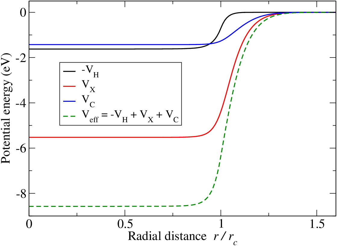
The ground state density is obtained by setting the center of mass variables to zero, i.e. and the bordering of the electron density to . The latter value corresponds to the minimum of the pseudo potential in Eq. (13). Several values of are given in the Table 1 for different nanoparticle sizes. The corresponding ground state densities and potentials are plotted, respectively, in Figs. 2 and 3. We notice that the electron density spreads at the border of the nanoparticle as expected. Moreover, the bordering parameter is proportional to the size of the nanoparticle and therefore the spreading of the electron density is almost the same for nanoparticles of different sizes. The exchange potential is three times larger than the Hartree and the correlation potentials, something that was already observed for thin metal films with DFT calculations [35]. We limit our study to nanoparticles between nm and nm. The lower value is constrained by the fact that for smaller nanoparticles quantum effects play a significant role in the electron dynamics [55]. For the upper limit, we are constrained by our Ansatz for the electron density that only includes the breathing and the dipole modes. Indeed multipolar modes should be also considered for larger nanoparticles [9].
Our model predicts the following plasmon resonance , which was obtained by evaluating the linear dipole frequency (14) at . Due to the spatial inhomogeneity of the electron density, the plasmon resonance increases with the size of the nanoparticle and in the limit of large nanoparticle, i.e. , tends to the bulk Mie frequency [9]. Thus, our model reproduces the expected blue shift of the resonant dipole frequency [56] that cannot be reproduced with a local Mie theory [57].
| [nm] | [at. u.] | [eV] | [eV] | |
| 1 | 248 | 8.46 | 5.05 | 0.37 |
| 1.5 | 836 | 10.95 | 5.10 | 0.27 |
| 2 | 1982 | 13.19 | 5.14 | 0.22 |
| 2.5 | 3870 | 15.24 | 5.15 | 0.19 |
We use a continuous laser field to excite the electron dynamics. The laser field propagates in the direction and is described by the following electric field: . The phase parameter allows us to describe different light polarizations going from linear polarization () to circular left () or right () polarization. We neglect the spatial variations of the electric field because the corresponding wavelength is much larger than the size of the nanoparticles.
In a first simulation, we excite the system with a circular right polarized field of intensity W/cm2, which corresponds to an electric field V/m. In all the simulations we took the laser frequency equal to the resonant dipole frequency of the system, , given in Table 1. We have checked that with such an intensity we are in the linear regime. The dipole responses and are given in Fig. 4. The results were obtained by solving the equations of motion (16)-(18) with a Runge-Kutta method of order . The dynamics is characterized by two regimes. During the first ten femtoseconds, one observes a transient regime in which the dipoles increase in amplitude. The typical timescale for this regime is given by the inverse of the damping parameter . After that, the system reaches a stationary regime, where the dipoles are oscillating with a phase shift of . We point out that, when one switches off the laser field, the dipoles behave as anharmonic damped oscillators, see Eqs. (17)-(18). Therefore, they will be exponentially damped on a time scale given by the inverse of the damping parameter .

Employing Eq. (10), we can directly compute the total orbital magnetic moment along the direction from the dipole responses and . The results are given in Fig. 5 for different polarizations of the incoming laser field, , and 0. We notice that in the case of a linearly polarized electric field, the total orbital magnetic moment remains zero. In this case one can check that both dipoles are oscillating in phase. However, if we use a circular right (black curve) or left (red curve) polarized field, then a net orbital magnetic moment is created in the system. This magnetic moment
increases during the transient regime until it reaches a stable value in the stationary regime. This situation corresponds to the case where the electric dipoles are oscillating with a phase offset
as pictured in Fig. 4. Moreover, one observes an opposite effect for circular left and circular right polarizations. Finally, if we excite the system with an elliptically polarized electric field (here ), then we still obtain a nonzero magnetic moment but smaller than the one obtained with full circular polarization. To summarize, in order to create a nonzero magnetic moment in gold nanoparticles, one has to excite the system at the resonant frequency of the surface plasmon. If one excites the system far from its resonance, then the dipoles will be significantly reduced as well as the magnetic moment. This is simply due to the fact that the dipole dynamics are described by nonlinear damped oscillators.

These observations are typical signatures of the inverse Faraday effect, where a part of the spin angular momentum of the light has been transferred to the electrons. An inverse Faraday effect has been predicted in a large gold nanoparticle [26] ( nm) using a full-wave electrodynamics solver (Lumerical) combined with individual electron motions. There, the authors have shown that the inverse Faraday effect emerges from an ensemble of solenoid-like motions for each electron inside the nanoparticle. In the next section, we propose a different explanation of the origin of the inverse Faraday effect observed in our system.
IV Mechanism of orbital magnetic moment generation
According to Eq. (10), the orbital magnetic moment is defined in terms of the electronic current density . The latter can be expressed as the product of the electron density and the electron mean velocity,
| (19) |
where the time-dependent electron density is defined in Eq. (8). The time dependence of the electronic current density is embedded in the dipole and breathing variables as well as in their time derivatives. It is straightforward to see that in the ground state the electronic current is zero. However, during the dynamics the spatial profile looks rather complicated especially near the surface of the nanoparticle.
In Fig. 6 we plot the current density vector field at a given time using the values of the dipoles obtained in Fig. 4. We only plot the and components of in the plane defined by since the component is exactly zero in this plane. We notice that almost all the vectors point in the same direction. This direction is defined by the instantaneous laser field and is changing in time since we excite the system with a circularly polarized electric field. The current density is strongest at the center of the nanoparticle and decreases rapidly at the border of the nanoparticle. From this plot, it is not easy to understand the origin of the orbital magnetic moment. It would seems that if we sum up all the contributions in the integral of Eq. (10) one obtains zero, but this is not the case. Notably in Fig. 6 the current density vector field is not centered around the origin but around the center of mass of the electrons . The latter enscribes a small circle around the center of the nanoparticle during one pulse oscillation. Mathematically speaking, this explains why the integral in Eq. (10) is not zero but adopts a finite value that depends on both dipole variables, and .
To have a better understanding of the underlying mechanism that is responsible for the generation of an orbital magnetic moment, let us define a time-averaged electron current density: . The time integration has to be done in the stationary regime over a full dipole period .


In Fig. 7 we plot the time-averaged current density corresponding to the same simulation as shown in Fig. 6. The averaged current density vanishes everywhere except at the surface of the nanoparticle. Moreover, the current density is rotating around the axis. This structure emerges from the superposition of many current densities that are all pointing in different directions defined by the instantaneous laser field. On average, they cancel everywhere except at the surface of the nanoparticle, because, as was mentioned before, each current is centered around the oscillating center of mass of the electrons. Thus, even though there are no real rotating surface currents, the system behaves as if that was the case. In the rest of this work, we will use the time average current density to evaluate the magnetic properties of the gold nanoparticles.


In Fig. 7 we have shown that the instantaneous current density can be mapped onto rotating surface currents. But that was only done in a given plane, defined by . In Fig. 8, we represent the time-averaged current density over the whole nanoparticle. We can recognize that the above assertion remains valid for the whole nanoparticle. This picture is particularly relevant to understand the behavior of the orbital magnetic moment shown in Fig. 5. If we change the polarization of the light from circular-right to circular-left, then the current will simply flow in the opposite direction and the induced magnetic moment will change its sign.
Finally, in Fig. 9 we analyze the intensity of the current density versus the radial distance from the axis [] in four different planes defined by , , , and , respectively. The radial profile is obtained by averaging the current density over the cylindrical angle. The current density is peaked around the surface of the nanoparticle, as expected. For instance, for , the peak is observed at . We further note that the current density is maximal in the plane and decreases progressively when one moves along the axis. The value of the electric current density is of the order of A/m2, which seems to be reasonable because it corresponds approximatively to a single electron crossing a surface of nm2 each femtosecond. However, this value depends mainly on the size of the nanoparticle and on the intensity of the laser excitation. This issue will be discussed in the next section.
V Nonlinear regime and size dependence
| [nm] | [A/m | [T] | |
| 1 | 1.85 | 10.4 | 0.019 |
| 1.5 | 3.41 | 65.2 | 0.030 |
| 2 | 4.93 | 228.1 | 0.053 |
| 2.5 | 6.45 | 599.9 | 0.071 |
All the results discussed in the previous sections were obtained for gold nanoparticles with a radius of nm and for laser excitations with an intensity of W/cm2. In this section, we study the influence of the nanoparticle size and of the laser intensities on the magnetic properties of the gold nanoparticles.
In Table 2, denotes the maximal value of the time-averaged current density, obtained at the surface of the nanoparticle for plane . We also provide the total magnetic moment and the magnetic field at the center of the nanoparticles for four different sizes. The magnetic field is calculated with the Biot-Savart law,
| (20) |
The numerical integration of Eq. (20) gives a static magnetic field at the center of the nanoparticle, such that one can use the time-average current density instead of the current density . We give the value of the magnetic field only at the center of the nanoparticle because it reaches it’s largest value at that particular position. The laser intensity remains equal to W/cm2 so that we are in the linear regime. The total magnetic moment and the magnetic field at the center of the nanoparticle are along the direction and can be positive or negative depending on whether the surface currents are rotating clockwise or counter-clockwise.

In Fig. 10 we investigate the size dependence of the different quantities given in Table 2. We observe that both the maximal current density and the magnetic moment per atom increase linearly with the radius of the nanoparticle. A similar trend is observed for the magnetic field at the center of the nanoparticle. The behaviors of the magnetic field and the magnetic moment can be understood from the behavior of the maximal current density by considering the integral over the surface of the nanoparticle in Eqs. (10) and (20). Note that the total magnetic moment scales as because the number of atoms in the nanoparticle scales as . This explains the large increase of the total magnetic moment seen in Table 2. Our model predicts an increase of the magnetic moment and the magnetic field with an increase of the size of the nanoparticle. However, this will not happen indefinitely. The reason, which was already mentioned before, is that for larger nanoparticles ( nm) we have a strong damping due to radiative losses, see Fig. 1. The latter may considerably reduce the amplitude of the dipoles and hence the amplitude of the magnetic moment and the magnetic field.

In Fig. 11 we study the influence of the laser intensity on the maximal current density, the magnetic moment per atom, and the magnetic field, respectively. The system is in the linear regime for the smallest intensity ( W/cm2), but not for the highest laser intensity ( W/cm2).
One observes that all quantities increase with the laser field, simply because
the electrons absorb more energy from the laser, which increases the dipole motion and thus the maximal current density. The total magnetic moment and the magnetic field follow the same trend as the current density. For small intensities, the magnetic moment increases linearly with the laser intensity and hence with , see Fig. 11(b). This again demonstrates that the generation of an orbital magnetic moment in our system is an orbital inverse Faraday effect.
Note that the magnetic field created at the center of the nanoparticle is static during the duration of the laser pulse and can reach considerable values ( T). In the nonlinear regime, the increase of the induced magnetic quantities starts leveling off.
Simulations performed at higher laser intensities (not shown here) reveal a saturation of all such quantities to a maximal value.
The quantities shown in Fig. 11 are probably overestimated for the largest laser intensity, especially when higher-order multipolar plasmon modes (quadrupole, octupole) start to play a significant role in the electron dynamics.
The reason is that our model is based on the assumption that the electron density remains isotropic during all the dynamics. Although this assumption can be justified in the linear regime, it is not necessarily valid in the strongly nonlinear regime. We expect that a more general description of the electron density, taking into account higher-order multipolar modes, will be more accurate in the nonlinear regime. Indeed the latter will break the spherical symmetry of the electron density and thus probably reduce the rotating surface currents. Moreover, other nonlinear effects such as ionization or generation of solitons [58], which cannot be described with our Ansatz, may lead to a different electron dynamics in the nonlinear regime.
VI Discussions and Conclusions
We have used a QHD model to show that, under the action of a circularly polarized laser field, gold nanoparticles can build up a static magnetic moment. We have shown that the induced magnetization per atom is proportional to the radius of the nanoparticle. The corresponding physical mechanism can be understood by analyzing the time-averaged electron current density, which exhibits rotating surface currents. The latter arise from collective effects described by the dipole and the breathing dynamics of the electron cloud. We have shown that this mechanism exhibits all the properties of a classical inverse Faraday effect: (i) the induced magnetization is static and reverses its sign when changing the light polarization from circular right to circular left, (ii) there is no induced magnetic moment for a linear polarization, and (iii) for small laser intensities the induced magnetization scales as the square of the electric field. We emphasize here the importance of the finite size of the system, which constitutes an essential ingredient for the generation of the magnetic moment. We would like to stress that in order to create a magnetic moment in gold nanoparticles, one has to excite the system at the resonant frequency of the surface plasmon. For excitations far off the plasmon resonance the magnetic moment remains close to zero.
In our model, a magnetic moment is created in gold nanoparticles by the collective motion of the electrons that interact with a circularly polarized laser field. This is in contrast with an earlier approach [26], where the authors analyzed that the magnetic moment emerges from an ensemble of independent solenoid-like motions for each electron. The QHD model employed in the present work goes beyond the independent and free-electron approximation by taking into account the main quantum many-body effects, such as the Hartree potential and the exchange and correlation effects. Using the same laser intensity, we predict an electronic current density four orders of magnitudes larger than in Ref. [26]. Although this difference is important, it is most probably due the different approach used in the two models. Indeed, in Ref. [26], the authors have assumed that the charge distribution in the nanoparticle stays uniform during the entire laser pulse and hence they neglect any redistribution of the electric field due to other nonlinear phenomena. On the contrary, in our model, the electric current responsible for the creation of an orbital magnetization is caused by the combination of the dipole motions (surface plasmons) and the inhomogeneity of the electron density at the surface of the nanoparticle (spill-out).
Summarizing, we have shown that surface plasmons support the generation of an orbital angular momentum in gold nanoparticles. This phenomenon corresponds to a transfer of the spin angular momentum of the light to the electronic orbital degree of freedom in the nanoparticle through the plasmonic orbital inverse Faraday effect. As a result, a static magnetic field is created inside the nanoparticle during the laser pulse. In future studies, it would be interesting to study other geometries such has nano-rings, since a resonant inverse Faraday effect was recently predicted in such nanostructures [27, 58]. The computed induced magnetic moments in the nanoparticle are quite large, of about 0.35 /atom for a laser intensity of W/cm2. Our study focused on gold nanoparticles but in principle other materials, such as silver or aluminium, could be investigated as well within the present theory. The decisive point for the magnetic moment generation is that the material supports a strong plasmonic response at the driving laser frequency. The thus-generated magnetic field could be employed as a new approach to achieve ultrafast plasmon-assisted all-optical switching in suitable systems such as core/shell nanoparticles, supported gold discs or gold rings with a magnetic core inside.
Acknowledgements.
We gratefully acknowledge valuable discussions with F. Haas, M. Berritta, A. Dmitriev, and V. Kapaklis. This work has been financially supported by the European Union’s Horizon2020 Research and Innovation Programme under Grant agreement No. 737709 (FEMTOTERABYTE, http://www.physics.gu.se/femtoterabyte), the Knut and Alice Wallenberg Foundation (Contract No. 2015.0060), the Swedish Research Council (VR), and the Swedish National Infrastructure for Computing (SNIC).References
- [1] G. Armelles, A. Cebollada, A. García-Martín, and M. Ujué González, Adv. Opt. Mater. 1, 10 (2013).
- [2] D. Bossini, V. I. Belotelov, A. K. Zvezdin, A. N. Kalish, and A. V. Kimel, ACS Photonics 3, 1385 (2016).
- [3] I. S. Maksymov, Rev. Phys. 1, 36 (2016).
- [4] P. K. Jain, Y. Xiao, R. Walsworth, and A. E. Cohen, Nano Lett. 9, 1644 (2009).
- [5] N. Maccaferri, A. Berger, S. Bonetti, V. Bonanni, M. Kataja, Q. H. Qin, S. van Dijken, Z. Pirzadeh, A. Dmitriev, J. Nogués, J. Åkerman, and P. Vavassori, Phys. Rev. Lett. 111, 167401 (2013).
- [6] E. Melander, E. Östman, J. Keller, J. Schmidt, E. T. Papaioannou, V. Kapaklis, U. B. Arnalds, B. Caballero, A. García-Martín, J. C. Cuevas, and B. Hjörvarsson, Appl. Phys. Lett. 101, 063107 (2012).
- [7] F. Pineider, G. Campo, V. Bonanni, C. de Julián Fernández, G. Mattei, A. Caneschi, D. Gatteschi, and C. Sangregorio, Nano Lett. 13, 4785 (2013).
- [8] E. Petryayeva and U. J. Krull, Anal. Chim. Acta 706, 8 (2011).
- [9] U. Kreibig and M. Vollmer, Optical properties of metal clusters (Springer, Berlin Heidelberg, 1995).
- [10] J. P. van der Ziel, P. S. Pershan, and L. D. Malmstrom, Phys. Rev. Lett. 15, 190 (1965).
- [11] P. S. Pershan, J. P. van der Ziel, and L. D. Malmstrom, Phys. Rev. 143, 574 (1966).
- [12] C. D. Stanciu, F. Hansteen, A. V. Kimel, A. Kirilyuk, A. Tsukamoto, A. Itoh, and Th. Rasing, Phys. Rev. Lett. 99, 047601 (2007).
- [13] S. Alebrand, M. Gottwald, M. Hehn, D. Steil, M. Cinchetti, D. Lacour, E. E. Fullerton, M. Aeschlimann, and S. Mangin, Appl. Phys. Lett. 101, 162408 (2012).
- [14] S. Mangin, M. Gottwald, C.-H. Lambert, D. Steil, V. Uhlir, L. Pang, M. Hehn, S. Alebrand, M. Cinchetti, G. Malinowski, Y. Fainman, M. Aeschlimann, and E. E. Fullerton, Nat. Mater. 13, 286 (2014).
- [15] C.-H. Lambert, S. Mangin, B. S. D. C. S. Varaprasad, Y. K. Takahashi, M. Hehn, M. Cinchetti, G. Malinowski, K. Hono, Y. Fainman, M. Aeschlimann, and E. E. Fullerton, Science 345, 1337 (2014).
- [16] M. S. El Hadri, P. Pirro, C.-H. Lambert, N. Bergeard, S. Petit-Watelot, M. Hehn, G. Malinowski, F. Montaigne, Y. Quessab, R. Medapalli, E. E. Fullerton, and S. Mangin, Appl. Phys. Lett. 108, 092405 (2016).
- [17] R. John, M. Berritta, D. Hinzke, C. Müller, T. Santos, H. Ulrichs, P. Nieves, J. Walowski, R. Mondal, O. Chubykalo-Fesenko, J. McCord, P. M. Oppeneer, U. Nowak, and M. Münzenberg, Sci. Rep. 7, 4114 (2017).
- [18] M. Vomir, M. Albrecht, and J.-Y. Bigot, Appl. Phys. Lett. 111, 242404 (2017).
- [19] R. Hertel, J. Magn. Magn. Mater. 303, L1 (2006).
- [20] M. I. Kurkin, N. B. Bakulina, and R. V. Pisarev, Phys. Rev. B 78, 134430 (2008).
- [21] S. R. Woodford, Phys. Rev. B 79, 212412 (2009).
- [22] D. Popova, A. Bringer, and S. Blügel, Phys. Rev. B 84, 214421 (2011).
- [23] M. Berritta, R. Mondal, K. Carva, and P. M. Oppeneer, Phys. Rev. Lett. 117, 137203 (2016).
- [24] I. D. Tokman and A. V. Shvetsov, Bull. Russ. Acad. Sci.: Physics 73, 28 (2009).
- [25] I. I. Smolyaninov, C. C. Davis, V. N. Smolyaninova, D. Schaefer, J. Elliott, and A. V. Zayats, Phys. Rev. B 71, 035425 (2005).
- [26] A. Nadarajah and M. T. Sheldon, Opt. Express 25, 12753 (2017).
- [27] K. L. Koshelev, V. Y. Kachorovskii, and M. Titov, Phys. Rev. B 92, 235426 (2015).
- [28] S. M. Hamidi, M. Razavinia, and M. M. Tehranchi, Opt. Commun. 338, 240 (2015).
- [29] T.-M. Liu, T. Wang, A. H. Reid, M. Savoini, X. Wu, B. Koene, P. Granitzka, C. E. Graves, D. J. Higley, Z. Chen, G. Razinskas, M. Hantschmann, A. Scherz, J. Stöhr, A. Tsukamoto, B. Hecht, A. V. Kimel, A. Kirilyuk, T. Rasing, and H. A. Dürr, Nano Lett. 15, 6862 (2015).
- [30] A. Dutta, A. V. Kildishev, V. M. Shalaev, A. Boltasseva, and E. E. Marinero, Opt. Mater. Express 7, 4316 (2017).
- [31] M. Kataja, F. Freire-Fernández, J. P. Witteveen, T. K. Hakala, P. Törmä, and S. van Dijken, Appl. Phys. Lett. 112, 072406 (2018).
- [32] G. Manfredi, Fields Inst. Commun. Series 46, 263 (2005).
- [33] S. V. Vladimirov and Y. O. Tyshetskiy, Physics-Uspekhi 54, 1243 (2011).
- [34] C. Ciracì and F. Della Sala, Phys. Rev. B 93, 205405 (2016).
- [35] N. Crouseilles, P.-A. Hervieux, and G. Manfredi, Phys. Rev. B 78, 155412 (2008).
- [36] C. Ciracì, Phys. Rev. B 95, 245434 (2017).
- [37] J. Hurst, F. Haas, G. Manfredi, and P.-A. Hervieux, Phys. Rev. B 89, 161111 (2014).
- [38] G. Toscano, J. Straubel, A. Kwiatkowski, C. Rockstuhl, F. Evers, H. Xu, N. Asger Mortensen, and M. Wubs, Nat. Commun. 6, 7132 (2015).
- [39] J. Hurst, K. Lévêque-Simon, P.-A. Hervieux, G. Manfredi, and F. Haas, Phys. Rev. B 93, 205402 (2016).
- [40] F. Haas, G. Manfredi, P. K. Shukla, and P.-A. Hervieux, Phys. Rev. B 80, 073301 (2009).
- [41] M. Brewczyk, K. Rza̧żewski, and C. W. Clark, Phys. Rev. Lett. 78, 191 (1997).
- [42] C. David and F. J. García de Abajo, J. Phys. Chem. C 115, 19470 (2011).
- [43] S. Raza, S. I. Bozhevolnyi, M. Wubs, and N. Asger Mortensen, J. Phys.: Condens. Matter 27, 183204 (2015).
- [44] A. V. Krasavin, P. Ginzburg, and A. V. Zayats, Laser & Photon. Rev. 12, 1700082 (2018).
- [45] A. D. Becke, Phys. Rev. A 38, 3098 (1988).
- [46] L. Brey, J. Dempsey, N. F. Johnson, and B. I. Halperin, Phys. Rev. B 42, 1240 (1990).
- [47] D. Michta, F. Graziani, and M. Bonitz, Contr. Plasma Phys. 55, 437 (2015).
- [48] M. Battiato, G. Barbalinardo, and P. M. Oppeneer, Phys. Rev. B 89, 014413 (2014).
- [49] The polylogarithm function is defined as , where , , and .
- [50] M. Quinten, Optical Properties of Nanoparticle Systems: Mie and Beyond (Wiley-VCH, Weinheim, 2011).
- [51] G. Weick, R. A. Molina, D. Weinmann, and R. A. Jalabert, Phys. Rev. B 72, 115410 (2005).
- [52] A. Derkachova, K. Kolwas, and I. Demchenko, Plasmonics 11, 941 (2016).
- [53] A. Brandstetter-Kunc, G. Weick, D. Weinmann, and R. A. Jalabert, Phys. Rev. B 91, 035431 (2015).
- [54] X. Li, D. Xiao, and Z. Zhang, New J. Phys. 15, 023011 (2013).
- [55] G. Weick, PhD Thesis, Université Louis Pasteur, Strasbourg. Available at http://www.theses.fr (2006).
- [56] C. Bréchignac, P. Cahuzac, J. Leygnier, and A. Sarfati, Phys. Rev. Lett. 70, 2036 (1993).
- [57] R. Ruppin, Phys. Rev. Lett. 31, 1434 (1973).
- [58] K. L. Koshelev, V. Y. Kachorovskii, M. Titov, and M. S. Shur, Phys. Rev. B 95, 035418 (2017).