Extremely Large Aperture Massive MIMO:
Low Complexity Receiver Architectures

Abolfazl Amiri,
Marko Angjelichinoski, Elisabeth de Carvalho Affiliation: Department of Electronic Systems
Aalborg University, Denmark
Email: {aba,maa,edc}@es.aau.dk Robert W. Heath Jr Affiliation: Department of Electrical and Computer Engineering
The University of Texas at Austin, TX, USA
Email: rheath@utexas.edu

Abstract

This paper focuses on new communication paradigms arising in massive multiple-input-multiple-output systems where the antenna array at the base station is of extremely large dimension (xMaMIMO). Due to the extreme dimension of the array, xMaMIMO is characterized by spatial non-stationary field properties along the array; this calls for a multi-antenna transceiver design that is adapted to the array dimension but also its non-stationary properties. We address implementation aspects of xMaMIMO, with computational efficiency as our primary objective. To reduce the computational burden of centralized schemes, we distribute the processing into smaller, disjoint sub-arrays. Then, we consider several low-complexity data detection algorithms as candidates for uplink communication in crowded xMaMIMO systems. Drawing inspiration from coded random access, one of the main contributions of the paper is the design of low complexity scheme that exploits the non-stationary nature of xMaMIMO systems and where the data processing is decentralized. We evaluate the bit-error-rate performance of the transceivers in crowded xMaMIMO scenarios. The results confirm their practical potential.

Index Terms:

Very large arrays, Massive MIMO, coded random access, non-stationary, 5G

I Introduction

Massive multiple-input-multiple-output (MIMO) is a key technology in cellular communication systems for increasing area spectral efficiency [1], [2]. The highest gains with massive MIMO are achieved when the antenna array dimension is very large [3, 4]. This has motivated the introduction of new types of deployment where arrays with extremely large dimension are deployed as part of a large infrastructure, for example along the walls of buildings in a mega-city, in airports, large shopping malls or along the structure of a stadium [4]. Similarly, large intelligent surfaces have emerged involving large electromagnetic surfaces [5]. Such a massive MIMO system with antenna arrays of extremely large dimension is denoted as xMaMIMO.

With increased antenna array dimensions, spatial non-wide sense stationary properties appear across the array due to electromagnetic propagation attributes as well as the distance between the users and the array that becomes smaller than the Rayleigh distance (see Fig. 1). In such xMaMIMO systems, different channel models and receiver algorithms are needed that account for this non-stationarity.

In this paper, we consider non-stationary properties through the concept of visibility region. A visibility region is associated to one given user and is defined as the portion of the array that one given user sees, i.e. that is able to receive signals from the user. This behaviour of the channel introduces an inherent sparsity to the system model, meaning that the transmitted signal of one user only exists on a small part of the antenna array. Thus, in contrast to ordinary massive MIMO models, user detection can be done by only processing the visibility region of each user. Using this important property of the system, we cut the computation costs of central processing, i.e. processing all antenna elements together, and propose local approaches. Note that the vast majority of the existing works on massive MIMO are based on conventional standard models with stationary characteristics of the channel [7]. In [8], an information theory study on non-wide sense stationary characteristics of massive MIMO channels is available where different parts of the array see different propagation paths. The problem of user assignment in large intelligent surfaces is studied in [9] in an interference-free environment.

To exploit cluster visibility regions, we propose new algorithms for uplink data detection. One of the challenges in xMaMIMO is its practical implementation, especially the enormous computational load that is required. To reduce the computation load of the system, we divide the array into smaller, disjoint units, referred to as subarrays and we distribute the computations among them. Then, we propose two types of uplink receivers. The first receiver is based on distributed linear data fusion (DLDF), where the users are first softly detected per subarray and then linearly fused in a centralized manner to produce the final soft information used to reconstruct the symbols. Next, relying on the non-stationary nature of the xMaMIMO system and drawing inspiration from coded random access, we propose a decentralized receiver of very low complexity where processing is executed locally per subarray with the fusion centre acting only as a forwarding node, relaying messages among the subarrays. One important factor here is the order of local processes and our proposed method copes delicately with it. The simulation results confirm the practical potential of the proposed receivers for xMaMIMO systems especially in crowded applications.

II System Model

We consider an xMaMIMO system. As discussed earlier, such infrastructure can be deployed along walls of buildings in urban sprawls, airports, shopping malls, even stadiums and they are envisioned to provide services to massive crowds.

A possible way to deal with the enormous computational load of the xMaMIMO system is to distribute the computation within separate processing units, referred to as subarrays. Depending on the specific implementation of the system and the actual physical constraints, a subarray can be defined in various ways. For instance, a subarray can correspond to a separate physical component. To see this, consider a large stadium. To provide high quality connectivity, an xMaMIMO system can be deployed along its walls. Depending on the actual deployment burden and cost, the operator might choose to mount individual arrays and connect them into a central processing unit using a cloud radio access network architecture. In such case, the number and the sizes of the subarrays is fixed. Alternatively, the operator might install a single array and provide logical interconnections between different portions of it. Here, the subarrays can be defined flexibly, adapting their size, number and position to the evolving data traffic conditions. We note that our framework is applicable to both cases as well as any combination in-between.

Let $M$ and $K$ denote the number of antennas and simultaneously active users, respectively. We assume narrow-band transmissions; $\mathbf{x}\in\mathbb{C}^{K}$ denotes the vector of complex input symbols, $\mathbf{H}\in\mathbb{C}^{M\times K}$ is the complex channel matrix and $\mathbf{n}\sim\mathcal{CN}(0,\sigma_{n}^{2}\mathbf{I}_{M})$ is the AWGN ( $\mathbf{I}_{M}$ denotes the identity matrix). We model the received baseband signal $\mathbf{y}\in\mathbb{C}^{M}$ across the whole array as follows:

\displaystyle\mathbf{y}=\mathbf{H}\mathbf{x}+\mathbf{n}.

(1)

Let $\mathbf{h}_{k}$ denote the $k$ -th column of $\mathbf{H}$ , corresponding to user $k$ ; in this work, we adopt the following channel model [6]:

\displaystyle\mathbf{h}_{k}=\sqrt{\mathbf{w}_{k}}\odot\bar{\mathbf{h}}_{k},

(2)

with $\odot$ denoting the element wise (Hadamard) products between two equal-size vectors. $\mathbf{w}_{k}$ captures the effect of large scale fading which in turn is a function of the distance of the user from the array, denoted with $\mathbf{d}_{k}$ , and the propagation properties of the environment; here, we employ the following simplified propagation model [11]:

\displaystyle\mathbf{w}_{k}=\beta\mathbf{d}^{\gamma}_{k},

(3)

where $\beta$ is a attenuation coefficient [11] and $\gamma$ is the pathloss exponent. $\bar{\mathbf{h}}_{k}\sim\mathcal{CN}(0,\mathbf{I})$ accounts for fast fading.

We split the xMaMIMO system into $B$ subarrays, each with $M^{(b)}\geq K,b=1,\ldots,B$ antennas such that $\sum_{b=1}^{B}M^{(b)}=M$ ; the received signal per subarrays is denoted by $\mathbf{y}^{(b)}\in\mathbb{C}^{M_{b}}$ and can be written as:

\displaystyle\mathbf{y}^{(b)}=\mathbf{H}^{(b)}\mathbf{x}+\mathbf{n}^{(b)},

(4)

for any $b=1,\ldots,B$ . Without loss of generality, in the rest of the paper we will assume that all active users transmit with equal power ( $E|x|^{2}=1$ ).

III Multiuser Detection Algorithms

In this section, we develop algorithms for multiuser symbol detection in xMaMIMO systems. Throughout, we assume perfect Channel State Information (CSI) at the receiver.

Refer to caption — Fig. 1: An example of extremely large M-MIMO array with spatial non-stationary regions along the array. Each user has a specific visibility region according to the channel conditions.

We distinguish between two different regimes of operation of the system: (i) stationary regime, where we assume that the users’ energy spread across the whole array (in other words, each user “sees” the whole array), and (ii) non-stationary regime, where we assume that the energy of each user is predominately concentrated on a limited number of antennas (see Fig. 1), which is usually significantly smaller than $M$ (i.e., each user “sees” only limited portion of the array). Obviously, the inherent, natural regime of operation of the system would be the non-stationary one in general, since the uplink power of each user will be unevenly distributed along the antenna array. Here, the distinction between the two regimes is done according to the knowledge of the receiver, i.e., when we say stationary regime, we mainly refer to the aspect of receiver agnosticism towards the non-stationary nature of the system.

III-A Stationary regime

III-A1 Centralized Zero-Forcing Receiver

Given the main underlying assumption, i.e., each user “reaches” every antenna of the array, a straightforward way to perform multiuser symbol detection is to process the complete received signal $\mathbf{y}$ . This can be done simply via Zero-Forcing (ZF); specifically, the ZF receiver for user $k$ , denoted by $\mathbf{F}_{ZF,k}$ , can be written as follows:

\displaystyle\mathbf{F}_{ZF,k}[\mathbf{H}]=\frac{\mathbf{h}^{H}_{k}\mathbf{P}^{\bot}_{\mathbf{\bar{H}_{k}}}}{\mathbf{h}^{H}_{k}\mathbf{P}^{\bot}_{\mathbf{\bar{H}_{k}}}\mathbf{h}_{k}},

(5)

with $\mathbf{P}^{\bot}_{\mathbf{\bar{H}_{k}}}=\mathbf{I}-\mathbf{\bar{H}_{k}}(\mathbf{\bar{H}_{k}}^{H}\mathbf{\bar{H}_{k}})^{-1}\mathbf{\bar{H}_{k}}^{H}$ [12]; $\mathbf{\bar{H}_{k}}$ is obtained from $\mathbf{H}$ by removing its $k^{th}$ column $\mathbf{h}_{k}$ . The post-processing SNR of the ZF receiver obtains the following form:

\displaystyle\text{SNR}_{ZF,k}=\rho\,\mathbf{h}^{H}_{k}\mathbf{P}^{\bot}_{\mathbf{\bar{H}_{k}}}\mathbf{h}_{k},

(6)

with $\rho={1}/{\sigma_{n}^{2}}$ . Given the extreme dimension of the aperture and potentially the extremely crowded setup, one should immediately note the computational burden of the centralized scheme. To reduce the computational complexity, we propose two schemes based on subarray processing. In both cases, the underlying idea is simple; instead of processing $\mathbf{y}$ fully, first process $\mathbf{y}^{(b)},b=1,\ldots,B$ and then perform linear soft fusion in a centralized manner.

III-A2 Distributed Linear Data Fusion Receiver

We introduce a simple, distributed linear data fusion (DLDF) method that combines softly the detected signals from each individual subarray. Furthermore, soft information of each user is obtained by

\displaystyle\hat{x}^{(b)}_{k}=\mathbf{F}_{ZF,k}[\mathbf{H}^{(b)}]\mathbf{y}^{(b)}

(7)

For each user $k$ we define the combined DLDF symbol $\hat{x}_{k}$ as follows:

\displaystyle\hat{x}_{k}

\displaystyle=\sum_{b=1}^{B}\alpha^{(b)}_{k}\hat{x}^{(b)}_{k},

(8)

where $\alpha^{(b)}_{k}$ is the weight for user $k$ using from subarray $b$ ; note that $\sum_{b=1}^{B}\alpha^{(b)}_{k}=1$ . It is worth mentioning that (8) is done in the central unit after receiving all the soft information from the subarrays. Also, mean squared error (MSE) of each user on subarrays is defined as:

\displaystyle\text{MSE}^{(b)}_{k}=E|{x}^{(b)}_{k}-\hat{x}^{(b)}_{k}|^{2}

(9)

where $E$ denotes the expectation operation. Here, it is taken with respect to the noise.

As the noise is assumed independent across subarrays, the overall MSE when data fusion is performed is:

\displaystyle\text{MSE}_{k}

\displaystyle=\sum_{b=1}^{B}\alpha^{(b)2}_{k}\text{MSE}^{(b)}_{k},

(10)

The objective is to minimize $\text{MSE}_{k}$ with the constraint $\sum_{b=1}^{B}\alpha^{(b)}_{k}=1$ . Using the Lagrange multiplier method [13] gives us the optimal weights:

\displaystyle\alpha^{(b)2}_{k}=\frac{\frac{1}{\text{MSE}^{(b)}_{k}}}{\sum_{b=1}^{B}\frac{1}{\text{MSE}^{(b)}_{k}}},

(11)

for $b=1,\ldots,B$ . Given that all users use equal transmit power, normalized to $1$ , we have that $\text{SNR}^{(b)}_{k}={1}/{\text{MSE}^{(b)}_{k}}$ , which yields:

\displaystyle\alpha^{(b)}_{k}=\frac{\text{SNR}^{(b)}_{k}}{\sum_{b=1}^{B}\text{SNR}^{(b)}_{k}}

(12)

for $b=1,\ldots,B$ . The complete algorithm is summarized in Algorithm 1.

Result: Estimates of

x_{k},k=1,\ldots,K

Initialize:

\mathbf{H},\>K,\>B,\>M^{(b)},\>\mathcal{K}=\left\{1,\ldots,K\right\}

Stage I: Distributed Linear Data Fusion (DLDF)

1. compute

\hat{x}^{(b)}_{k},k\in\mathcal{K},b=1,\ldots,B

via (7)

2. compute

\alpha_{k}^{(b)},k\in\mathcal{K},b=1,\ldots,B

via (12)

3. compute

\hat{x}_{k},k\in\mathcal{K}

via (8)

4. perform hard decision over

\hat{x}_{k},k\in\mathcal{K}

and terminate

Algorithm 1 Distributed Linear Data Fusion receiver.

III-B Non-stationary regime

In this case, we assume that the users have a limited visibility region of the array, which is illustrated in Fig. 1. Hence, the non-stationary regime of operation can be seen as a special case of the stationary one, implying that we can easily apply any of the receivers described in the previous subsection.

Nevertheless, we introduce a simple method, inspired from the concept of coded random access in slotted aloha IoT systems. They key idea operates as follows: given the non-stationary nature of the array, each user is predominantly present only on very limited number of subarrays, i.e., all of its power is concentrated over limited number of subarrays. As a result, the system becomes inherently sparse, implying that the subarrays where a user is not present should not be processed for that specific user. So, in principle, we can obtain a sparse bipartite graph, representing the connections of the users to the subarrays after which we can apply the principles of successive elimination of connections from the graphs as in coded random access. This further reduces the computational cost but since we are neglecting some portion of the signal energy, $p_{0}$ , and treat it as interference at the remaining arrays, and we do not perform any soft fusion at the central processing unit, it is reasonable to expect that the performance of the method might be slightly degraded in some configuration regions of the system (i.e., specific values of $K$ relative to $B$ and $M_{b},b=1,\ldots,B$ ).

Result:

\mathcal{H}

Initialize:

\mathbf{H},\>K,\>B,\>M_{b},\>p_{0},\>\mathcal{H}=\{0\}^{B\times K},\>\mathcal{B}=\left\{1,\ldots,B\right\}

for $k=1$ to $K$ do

1. reinitialize

p_{k}=0

2. compute total cumulative power

P_{k}

3. compute per subarray power

P_{k}^{(b)},b\in\mathcal{B}

while $p_{k}\leq p_{0}\cdot P_{k}$ do

1. find

b^{*}=\max_{b\in\mathcal{B}}P_{k}^{(b)}

p_{k}=p_{k}+P_{k}^{(b^{*})}

3. set

\mathcal{H}(b^{*},k)=1

\mathcal{B}=\mathcal{B}\setminus{{b}^{*}}

end while

end for

Algorithm 2 Bipartite graph construction from

\mathbf{H}

The most attractive feature of the proposed method is the fact that the bipartite graph can be constructed very simply, exploiting the sheer fact that the receiver has perfect CSI, i.e., it knows $\mathbf{H}$ ; in other words, by observing the $k$ -th column, the receiver can determine which parts of the array the dominant part of the power of user $k$ is allocated. This way, the receiver obtains a binary matrix $\mathcal{H}\in\{0,1\}^{B\times K}$ . We use $\mathcal{H}$ to construct a bipartite graph. Note that, at the beginning of the algorithm 3, the central unit runs Algorithm 2 according to the CSI and then sends the order of the detection to each subarray. This means that each subarray receives a schedule consisting of the list of users that should be detected by that subarray. This is the only centralized broadcasting in this algorithm and the rest of it is decentralized.

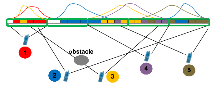
The procedure is described in Algorithm 2. Moreover, an example of xMaMIMO with 5 users is illustrated in Fig. 2 where the energy distribution of each user on antenna arrays is also presented. The equivalent bipartite graph representation of this setup is shown in Fig. 3 (a). The extension of this binary graph to a weighted one, where the weights show the portion of user’s total power, is left for future work.

The bipartite graph constructed this way is characterized by the following quantities: (i) a set $\mathcal{B}$ of $B$ nodes representing subarray units, (ii) a set $\mathcal{K}$ of $K$ user nodes and, (iii) a set $\mathcal{E}$ of edges, i.e. connection between users and subarrays. We use $\mathcal{G}=(\mathcal{B},\mathcal{K},\mathcal{E})$ to denote this graph. We also define the node degrees $S_{b},b\in\mathcal{B}$ and $U_{k},k\in\mathcal{K}$ ; the degrees give the number of edges connected to each of the nodes in $\mathcal{B}$ and $\mathcal{K}$ , respectively. For instance in Fig. 3(a), subarray $b=1$ only receives signal from user $k=1$ and user $k=3$ ; therefore, its degree is $S_{1}=2$ .

Once the graph has been constructed, we apply simple symbol detection strategy inspired from coded random access [10]. Hence, we search for subarrays with the lowest number of users; we detect the symbols of those users and subsequently remove them from the other subarrays. An illustrative example for the procedure is shown in Fig. 3. We assume xMaMIMO system with $K=5$ users and $B=5$ subarrays with graph representation shown in Fig. 3(a). After computing the degrees, we see that $S_{2}=1$ . Thus, we start signal detection in subarray $b=2$ for user $k=2$ . Then, we remove any other edges corresponding to user $k=2$ from the graph. We repeat the procedure for $S_{5}$ and $U_{5}$ in Fig. 3(b). In step (c), we have three nodes with same degree and similar conditions. We randomly choose $S_{3}$ and start a ZF detection within subarray $b=3$ between users $k=3$ and $k=4$ . After recovering both of them, we remove all edges from the graph corresponding to those users. Finally, in part (d) we have a singleton node that can be easily detected. Now, since all the users are detected, the algorithm terminates. The complete algorithm is summarized in Algorithm 3.

Result: Estimates of

x_{k},k=1,\ldots,K

Initialize:

\mathbf{H},\>K,\>B,\>M_{b}

\mathcal{B}=\{1,\ldots,B\},\>\mathcal{K}=\{1,\ldots,K\}

1. compute

\mathcal{H}

via Algorithm 2

while $\mathcal{K}\neq\emptyset$ do

1. compute node degrees

S_{b},b\in\mathcal{B}

U_{k},k\in\mathcal{K}

2. find

b^{*}=\min_{b\in\mathcal{B}}\left\{S_{b}\right\}

if $b^{*}=1$ (only user $k^{*}$ in the subarray with minimal degree) then

1. compute

\hat{x}_{k^{*}}^{(b^{*})}

via (7)

2. broadcast

\hat{x}_{{k}^{\dagger}}

so other subarrays remove it from

\mathbf{y}^{(b)}

for

b\in\mathcal{B}\setminus b^{*}

\mathcal{K}=\mathcal{K}\setminus{k^{*}}

if $b^{*}>1$ (multiple users $\mathcal{K}^{*}\subset\mathcal{K}$ in the subarray with minimal degree) then

while $\mathcal{K}^{*}\neq\emptyset$ do

1. sort the users according to

\text{SNR}_{ZF,k},k\in\mathcal{K}^{*}

in (6)

2. find

k^{\dagger}=\max_{k\in\mathcal{K}}\text{SNR}_{ZF,k}

3. broadcast

\hat{x}_{{k}^{\dagger}}

so all subarrays remove it from

\mathbf{y}^{(b)}

for

b\in\mathcal{B}

\mathcal{K}^{*}=\mathcal{K}^{*}\setminus{{k}^{\dagger}}

end while

\mathcal{K}=\mathcal{K}\setminus{\mathcal{K}^{*}}

end while

Algorithm 3 Low complexity multiuser detection in non-stationary regime

IV Complexity, Convergence and Delay Analyses

In this section we first consider computation complexity comparison between the proposed algorithm and the linear data fusion using ZF detector. Convergence and delay characteristics of the proposed algorithms are discussed next.

IV-A Complexity of DLDF

In DLDF we have three phases for user detection which have the following complexities:

1.

Data detection: Consists of ZF matrix inversion for all users in all of the subarrays with $M_{b}K$ elements, which have a complexity order of $BK(K)^{3}$ .
2.

SNR extraction: This function is also for all users in all of the subarrays containing $BK(M_{b}(K-1))$ .
3.

Soft fusion: The last part with $BK$ matrix multiplications.

IV-B Complexity of Algorithm 3

We study this part with two extreme cases that could happen regarding the nature of non-stationarity.

IV-B1 Worst case

This case occurs when we have all of the users in all of the subarrays or when we have them in only one subarray. Thus, the algorithm sets $\min N_{s}=K$ and performs detection over only one subarray. Moreover SNR extraction is also done for all users in this subarray containing $K(M_{b}(K-1))$ . Therefore, the complexity of this part is at most $K^{4}+K(M_{b}(K-1))$ calculations.

IV-B2 Best case

This case happens when we have users evenly distributed between subarrays meaning that each subarray performs detection over $\frac{K}{B}$ users. Therefore the complexity of the detection part is

\displaystyle B\left[\left(\frac{K}{B}\right)^{3}+\left(\frac{K}{B}-1\right)^{3}+\dots+1\right]<\frac{K^{4}}{B^{3}}.

(13)

Also, for the ordering part we have $\frac{KM_{b}K}{B}$ computations. TABLE I provides the complexity comparison between the aforementioned algorithms.

A rough comparison between the complexities of the Algorithms reveals that the complexity reduction of Algorithm 3 scales with $B$ in the worst case and with $B^{4}$ in the best case. If $B$ is of the order of $10$ , we see that significant computational power can be saved by employing Algorithm 3.

TABLE I: Complexity comparison of the studied methods

Methods	Number of multiplications
ZF-DLDF	$BK(K)^{3}+BK((K-1))+BK$
Algorithm 3	Worst case: $K^{4}+K(M_{b}(K-1))$
	Best case: ${K^{4}}B^{-3}+\frac{KM_{b}K}{B}$

IV-C Convergence Analyses

The analyses for the convergence for Algorithm 3 over graphical model can be found in [10]. Moreover, considering this algorithm as an extension to the model in [10] by enabling continuous signal space, i.e. we recover a part of data at each step even on non-singleton nodes, it will converge even faster due to this claim.

IV-D Delay Characteristics

In order to highlight the trade-off between using our proposed algorithms instead of the centralized methods, we discuss delay properties of the algorithms. Algorithm 3 introduces some delay due to the sequential nature of the algorithm. For example, while a selected subarray $b$ performs the detection of a given symbol, the other subarrays carrying the same symbol should wait for the input from subarray $b$ to perform interference cancellation.

This waiting time vanishes when we have sparse channels since different subarrays become independent as they involve different users. Thus, they can work together in a parallel mode. A deeper analysis of the overall delay is left for future work.

V Simulation Results

In this section we compare the Bit Error Rate (BER) performance of the proposed algorithm and DLDF. We assume a linear xMaMIMO configuration (see Fig. 2) for our simulations setup. We use Monte-Carlo simulations to generate the channel realizations. Some of the fixed variables are: $\beta=1$ , $\gamma=2$ , array length $=100$ m, power threshold for constructing the bipartite graph $p_{0}=0.9$ and we use an 8-PSK input constellation. Moreover, we assume that the user location has a random uniform distribution along the array. Note that user distribution and antenna array length have a direct impact on the large scale fading characteristics and therefore control the bipartite graph structure.

Fundamentally, for a given average user load per subarray, the BER performance is determined by the dimension of the visibility region seen by each user. Here, the users are at the same distance and uniformly distributed along the array, so that the average size of the visibility region is the same per user (except for users at the edges which have a non-significant impact for a large enough number of users). In the simulation, we study the following factors: a) the number of subarrays, b) the total number of users and c) the number of antenna per subarray.

First, we compare the BER of the detection methods for different numbers of subarrays, $B$ , while the number of antennas is fixed, $M=512$ , starting from a number of 2 subarrays (256 antennas per subarray) and ending by a number of 32 subarrays (16 antennas per subarray). We observe:

•

Algorithm 3 performs significantly better than the DLDF.
•

Linear processing: when the number of antennas per subarray is asymptotically large, due to the law of large numbers, the processing decouples across the subarrays (this fact is supported by the rich scattering assumption). Subarray processing becomes equivalent to a centralized linear processing. We observe an almost stable performance level (corresponding to the centralized processing) until a number of antennas per subarray smaller then 32.
•

Algorithm 3: the performance of algorithm 3 is degraded when the number of subarray is small. The reason is that the algorithm lacks degrees of freedom for the SIC mechanism to have its full effect. Performance saturates when the resolution offered by the number of subarrays reflects the non-stationarity patterns, more precisely when each subarray offers a stationary picture of the received signal.

In Fig. 5, we compare the performance of Algorithm 3 and DLDF with respect to the number of users. The total array size is kept fixed. The array is comprised of $B$ subarrays, each with a number of antennas $M_{b}=K$ . Note that the subarrays are not adjacent in this simulation. We make the following observations:

•

Again, algorithm 3 performs significantly better than the DLDF.
•

As the number of antennas grows at the same speed as the number of users, the user load per subarray is maintained so that performance remains approximately constant.
•

We observe an improvement of algorithm 3 as the granularity increases, i.e. the number of subarrays.

VI Conclusions

In a massive MIMO systems with extremely large arrays, users can effectively communicate only with a sub-part of the array called a visibility region. A receiver design should be adapted to this kind of non-stationary patterns with partially overlapping visibility regions. The receiver architectures proposed in this paper are based on subarray processing where part of the computational load is carried out. A central unit coordinates the operations at each subarray and proceeds to data fusion. We proposed a linear data fusion method, as well as a graph-based algorithm inspired from coded random access which uses low complexity and distributed scheme for the data detection. This method converts the propagation environment of the channel into a bipartite graph and detects the users in a novel scheme.

References

[1] F. Boccardi, R. W. Heath, A. Lozano, T. L. Marzetta and P. Popovski, ”Five disruptive technology directions for 5G,” in IEEE Communications Magazine, vol. 52, no. 2, pp. 74-80, Feb. 2014.
[2] E. G. Larsson, O. Edfors, F. Tufvesson and T. L. Marzetta, ”Massive MIMO for next generation wireless systems,” in IEEE Communications Magazine, vol. 52, no. 2, pp. 186-195, Feb. 2014.
[3] X. Gao and F. Tufvesson and O. Edfors, ”Massive MIMO channels - Measurements and models” 2013 Asilomar Conference on Signals, Systems and Computers, pp. 280-284, Nov. 2013.
[4] A.O. Martinez, E. de Carvalho , J. Nielsen, ”Towards very large aperture massive MIMO: A measurement based study”, in 2014 IEEE Globecom Workshops (GC Wkshps), pp. 281-286, Dec 2014.
[5] S. Hu and F. Rusek and O. Edfors , ”Beyond Massive MIMO: The Potential of Positioning With Large Intelligent Surfaces”, IEEE Transactions on Signal Processing, vol. 66, no. 7, pp. 1761-1774, Apr. 2018.
[6] H. Q. Ngo, E. G. Larsson and T. L. Marzetta, ”Energy and Spectral Efficiency of Very Large Multiuser MIMO Systems,” in IEEE Transactions on Communications, vol. 61, no. 4, pp. 1436-1449, Apr. 2013.
[7] T. L. Marzetta, ”Noncooperative Cellular Wireless with Unlimited Numbers of Base Station Antennas,” in IEEE Transactions on Wireless Communications, vol. 9, no. 11, pp. 3590-3600, Nov. 2010.
[8] X. Li, S. Zhou, E. Björnson and J. Wang, ”Capacity Analysis for Spatially Non-Wide Sense Stationary Uplink Massive MIMO Systems,” in IEEE Transactions on Wireless Communications, vol. 14, no. 12, pp. 7044-7056, Dec. 2015.
[9] S. Hu, K. Chitti, F. Rusek and O. Edfors, ”User Assignment with Distributed Large Intelligent Surface (LIS) Systems.” arXiv preprint arXiv:1709.01696, 2017.
[10] G. Liva, ”Graph-based analysis and optimization of contention resolution diversity slotted ALOHA”, IEEE Transactions on Communications, vol. 59, no. 2, pp. 477-487, Nov. 2011.
[11] D. Tse and P.Viswanath,”Fundamentals of Wireless Communication”, Cambridge University Press, New York, NY, USA, 2015.
[12] Tim Brown, Elisabeth De Carvalho and Persefoni Kyritsi, ”Practical guide to MIMO radio channel: With MATLAB examples”, John Wiley & Sons, 2012.
[13] S. Boyd and L. Vandenberghe, ”Convex optimization”, Cambridge university press, 2004.

Extremely Large Aperture Massive MIMO: Low Complexity Receiver Architectures

Abstract

Index Terms:

I Introduction

II System Model

III Multiuser Detection Algorithms

III-A Stationary regime

III-A1 Centralized Zero-Forcing Receiver

III-A2 Distributed Linear Data Fusion Receiver

III-B Non-stationary regime

IV Complexity, Convergence and Delay Analyses

IV-A Complexity of DLDF

IV-B Complexity of Algorithm 3

IV-B1 Worst case

IV-B2 Best case

IV-C Convergence Analyses

IV-D Delay Characteristics

V Simulation Results

VI Conclusions

References

Extremely Large Aperture Massive MIMO:
Low Complexity Receiver Architectures