General drawdown of general tax model in a time-homogeneous Markov framework

Our paper is part of a larger program to improve the control of a reserves/risk process $X$. The rough idea is that when below low levels $a$, the reserves should be replenished at some cost, and when above high levels $b$, the reserves should be invested to yield dividends – see for example [1]. The low levels first considered historically have been those of $X$, but one may equally consider low levels of the drawdown/regret/process reflected at the maximum, defined by

$$D_{t}=\overline{X}_{t}-X_{t},\hskip 10.00002pt\overline{X}_{t}:=\sup_{0\leq s\leq t}X_{s},$$

which turn out to be of interest in several problems in statistics, mathematical finance and risk theory [22, 25, 16, 23, 7, 12, 21, 17, 18, 9, 20, 8]. The book[26] summarizes most of the recent developments on drawdown.

Assume from now on that our underlying process $X$ is time-homogeneous and Markovian. The first passage times of $X$ across a level $x\in\mathbb{R}$ are denoted by

$$\tau_{x}^{+}=\inf\left\{t\geq 0:X_{t}>x\right\}\text{ and }\tau_{x}^{-}=\inf\left\{t\geq 0:X_{t}<x\right\}.$$

For simplicity, we assume $X$ is upward skip-free. Moreover, we assume $X$ is regular in the sense that $\mathbb{P}_{y}(\tau_{x}^{+(-)}<\infty)>0$, for all $x,y\in\mathbb{R}$.

Instrumental in achieving the control of one dimensional risk processes are the distributions of the two-sided smooth and non-smooth first passage times from a bounded interval $[u,v]$. For upward skip-free processes, it turns out easier to study the corresponding Laplace transforms:

	$\displaystyle B^{(q)}(x;u,v)$	$\displaystyle:=\mathbb{E}_{x}\left[e^{-q\tau_{v}^{+}}1_{\left\{\tau_{v}^{+}<\tau_{u}^{-}\right\}}\right],$		(1.1)
	$\displaystyle C^{(q,s)}(x;u,v)$	$\displaystyle:=\mathbb{E}_{x}\left[e^{-q\tau_{u}^{-}-s(u-X_{\tau_{u}^{-}})}1_{\left\{\tau_{u}^{-}<\tau_{v}^{+}\right\}}\right],$		(1.2)

where $q,s\geq 0$, and $u\leq x\leq v$. Indeed, for Lévy processes for example it holds that:

$$B^{(q)}(x;u,v)=\frac{W_{q}(x-u)}{W_{q}(v-u)},$$

where $W_{q}(x)$ is called the scale function [24, 11, 14], and for some non-homogeneous spectrally negative Markov processes [13] a similar formula holds

$$B^{(q)}(x;u,v)=\frac{W_{q}(x;u)}{W_{q}(v;u)},$$

where now the newly defined scale function naturally depends on the two variables $x,u$.

Several control problems for $(X,D)$ are known to reduce to the study of the process $\overline{X}_{t}$ with all its negative excursions excised, which turns out to be a deterministic process, killed at a random time [3, 2]–see Figure 1 below. This supports the parallel fundamental idea of [18] to base the study of $(X,D)$ on the existence of two differential parameters.

A necessary condition for Assumption 1.1 to hold is that

$$\tau_{x}^{+}=0\mbox{ and }X_{\tau_{x}^{+}}=x,\mathbb{P}_{x}-a.s.\mbox{ for all }x\in\mathbb{R}.$$

To understand the joint dynamics of two dimensional process $t\mapsto(X_{t},D_{t})$, it is useful to look at Figure 1, reproduced from [8], which depicts a sample path of $(X,D)$, where $X$ is chosen to be the standard Brownian motion and the exit region is $R=[-6,7]\times[0,10]$.

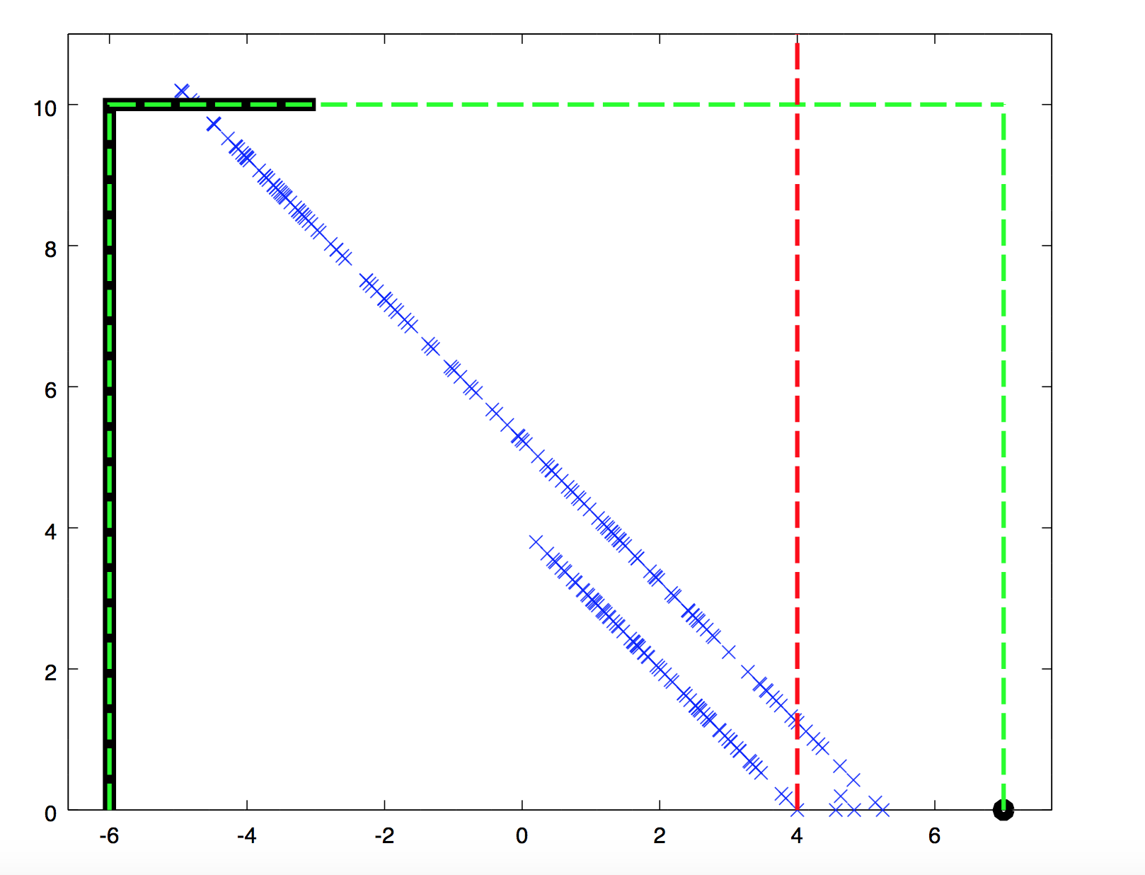
As is clear from the figure and from its definition, the process $(X,D)$ has very particular dynamics on $R$: away from the boundary $\partial_{1}:=\{x\in{\mathbb{R}}\times{\mathbb{R}}_{+}:x_{2}=0\}$ it oscillates on the line segment $L_{\overline{X}_{t}}$ where, for $c\in{\mathbb{R}}$, $L_{c}:=\{x\in{\mathbb{R}}\times{\mathbb{R}}_{+}:x_{1}+x_{2}=c\}$. These oblique lines represent each a negative excursion. On $\partial_{1}$, we observe the evolution of the process $\overline{X}_{t}$ with all its negative excursions excised; as $\overline{X}_{t}$ increases, the line segment $L_{\overline{X}_{t}}$ on which $(X,D)$ oscillates during a negative excursion advances continuously to the right.

To fully specify the process $\overline{X}_{t}$ with its negative excursions excised, we must give a rule for killing a negative excursion; two classic choices are $X_{t}<a$ (ruin stopping) and $D_{t}>d$ (drawdown stopping), which are the left and upper boundaries in Figure 1, respectively. A linear combination of these, translating into an oblique upper boundary, has been studied in [9].

In our paper we consider more general upper boundaries, which include the previous works as particular cases. Following [20], we consider stopping times

$$\tau_{f}=\inf\left\{t\geq 0:X_{t}<f(\overline{X}_{t})\right\}=\inf\{t\geq 0:Y_{t}>0\},$$

where

$$Y_{t}=f(\overline{X}_{t})-X_{t}=D_{t}-\overline{f}(\overline{X}_{t}),\;{t\geq 0}$$

will be called a general drawdown process. Here $\overline{f}(m):=m-f(m)$, and $f$ must be nondecreasing such that

$$f(x)<x\Leftrightarrow\overline{f}(x)>0,\hskip 10.00002ptx\in\mathbb{R}\text{.}$$

Note that we have $Y_{0}=f(X_{0})-X_{0}<0$.

General drawdown times include many important particular subcases which have been extensively studied in the literature:

1. 1.

   If $f(x)=0$, $\tau_{f}=\tau_{0,0}$ is the ruin time.

2. 2.

   If $f(x)=x-d$, $\tau_{f}=\tau_{1,d}$ is the classic drawdown time.

3. 3.

   If $f(x)=\xi x,\xi<1$, when $\tau_{f}=\tau_{\xi,0}$ is the proportional drawdown time.

4. 4.

   If

   $$f(x)=\xi x-d\Leftrightarrow\bar{f}(m)=m-f(m)=(1-\xi)m+d,\;\xi\in{(-\infty,1]},d\geq 0,(1-\xi)>0,$$

   (1.3)

   the corresponding drawdown time is

   $$\tau_{f}=\tau_{\xi,d}=\inf\left\{t\geq 0:X_{t}\leq\xi\overline{X}_{t}-d\right\}=\inf\left\{t\geq 0:\overline{X}_{t}-X_{t}>(1-\xi)\overline{X}_{t}+d\right\}.$$

   (1.4)

   This is called the affine drawdown studied in [9]. It turns out that this extension complicates only slightly the classic drawdown results, while allowing treating simultaneously times cases 2 and 3.

5. 5.

   Nonlinear drawdown times emerged in [16] and were used by Azéma and Yor [10] to provide a solution of the Skorokhod problem of stopping a Brownian motion to obtain a given desired centered marginal measure.

Contents. Below, we extend first the general drawdown results of [20] from spectrally negative Lévy processes to spectrally negative time-homogeneous Markov processes – see Section 2. Then, in Section 3 we allow also for the possibility of general taxation. The method of proof involves a nontrivial use of the “differential exit problems” of [18]. The results in Section 2 are applied in the three particular cases in which the “differential exit parameters” of [18] are analytically computable: spectrally negative Lévy processes and diffusions. A third example, which is illustrated in [18], is of Ornstein-Uhlenbeck-type processes with exponential jumps.

The following pathwise inequalities are central to the construction of tight bounds for the joint law of the triplet $(\tau_{f},\overline{X}_{\tau_{f}},Y_{\tau_{f}})$.

On the other hand, by using the same argument, we have, $\mathbb{P}_{x}$-a.s.,

$$(\tau_{f(x)}^{-}<\tau_{x+\varepsilon}^{+})=(\tau_{f}\leq\tau_{f(x)}^{-}<\tau_{x+\varepsilon}^{+})\subset(\tau_{f}<\tau_{x+\varepsilon}^{+}),$$

(2.4)

and

$$(\tau_{f}<\tau_{x+\varepsilon}^{+})=(\tau_{f(x+\varepsilon)}^{-}\leq\tau_{f}<\tau_{x+\varepsilon}^{+})\subset(\tau_{f(x+\varepsilon)}^{-}<\tau_{x+\varepsilon}^{+}).$$

(2.5)

For any path $\omega\in(\tau_{f(x)}^{-}<\tau_{x+\varepsilon}^{+})$, we know from (2.4) that $\omega\in(\tau_{f}\leq\tau_{f(x)}^{-}<\tau_{x+\varepsilon}^{+})$. This implies $\overline{X}_{\tau_{f}}(\omega)\leq x+\varepsilon$ and $X_{\tau_{f}}(\omega)\geq X_{\tau_{f(x)}^{-}}(\omega)$, which further entails that $Y_{\tau_{f}}(\omega)=f(\overline{X}_{\tau_{f}}(\omega))-X_{\tau_{f}}(\omega)\leq f(x+\varepsilon)-X_{\tau_{f(x)}^{-}}(\omega)$. Therefore, by the above analysis and (2.4),$\hskip 10.00002pt\mathbb{P}_{x}$-a.s.,

$$e^{-q\tau_{f(x)}^{-}-s(f(x+\varepsilon)-X_{\tau_{f(x)}^{-}})}1_{\left\{\tau_{f(x)}^{-}<\tau_{x+\varepsilon}^{+}\right\}}\leq e^{-q\tau_{f}-sY_{\tau_{f}}}1_{\left\{\tau_{f}<\tau_{x+\varepsilon}^{+}\right\}}$$

which naturally leads to (2.2).

Similarly, for any sample path $\omega\in(\tau_{f}<\tau_{x+\varepsilon}^{+})$, we know from (2.5) that $\omega\in(\tau_{f(x+\varepsilon)}^{-}\leq\tau_{f}<\tau_{x+\varepsilon}^{+})$, which implies that $f(x)-X_{\tau_{f(x+\varepsilon)}^{-}}(\omega)\leq Y_{\tau_{f(x+\varepsilon)}^{-}}(\omega)\leq Y_{\tau_{f}}(\omega)$. Here the last inequality is because $Y_{\tau_{f(x+\varepsilon)}^{-}}(\omega)\leq 0\leq Y_{\tau_{f}}(\omega)$ if $\tau_{f(x+\varepsilon)}^{-}<\tau_{f}$, and $Y_{\tau_{f(x+\varepsilon)}^{-}}(\omega)=Y_{\tau_{f}}(\omega)$ if $\tau_{f(x+\varepsilon)}^{-}=\tau_{f}$. Therefore, we obtain,$\hskip 10.00002pt\mathbb{P}_{x}$-a.s.,

$$e^{-q\tau_{f}-sY_{\tau_{f}}}1_{\left\{\tau_{f}<\tau_{x+\varepsilon}^{+}\right\}}\leq e^{-q\tau_{f(x+\varepsilon)}^{-}-s(f(x)-X_{\tau_{f(x+\varepsilon)}^{-}})}1_{\{\tau_{f(x+\varepsilon)}^{-}<\tau_{x+\varepsilon}^{+}\}},$$

which proves (2.3).

 

By Proposition 2.1, we easily obtain the following useful estimates.

Next we present our main results of the general drawdown.

Similarly, let

$$h(x)=\mathbb{E}_{x}\left[e^{-q\tau_{f}-sY_{\tau_{f}}}1_{\{\overline{X}_{\tau_{f}}\leq K\}}\right],\hskip 10.00002ptx<K.$$

By the strong Markov property of $X$ at maxima, for any $X_{0}=x\leq y<K$ and $0<\varepsilon<K-y$, we have

$$h(y)=\mathbb{E}_{y}\left[e^{-q\tau_{f}-sY_{\tau_{f}}}1_{\left\{\tau_{f}<\tau_{y+\varepsilon}^{+}\right\}}\right]+\mathbb{E}_{y}\left[e^{-q\tau_{y+\varepsilon}^{+}}1_{\{\tau_{y+\varepsilon}^{+}<\tau_{f}\}}\right]h(y+\varepsilon).$$

By Corollary 2.1, it follows that

$$\left\{\begin{array}[c]{c}h(y)\leq e^{s(f(y+\varepsilon)-f(y))}C^{(q,s)}(y;f(y+\varepsilon),y+\varepsilon)+B^{(q)}(y;f(y),y+\varepsilon)h(y+\varepsilon),\\ h(y)\geq e^{-s(f(y+\varepsilon)-f(y))}C^{(q,s)}(y;f(y),y+\varepsilon)+B^{(q)}(y;f(y+\varepsilon),y+\varepsilon)h(y+\varepsilon).\end{array}\right.$$

It follows that

$$\left\{\begin{array}[c]{l}h(y+\varepsilon)-h(y)\geq-e^{s(f(y+\varepsilon)-f(y))}C^{(q,s)}(y;f(y+\varepsilon),y+\varepsilon)+\left[1-B^{(q)}(y;f(y),y+\varepsilon)\right]h(y+\varepsilon),\\ h(y+\varepsilon)-h(y)\leq-e^{-s(f(y+\varepsilon)-f(y))}C^{(q,s)}(y;f(y),y+\varepsilon)+\left[1-B^{(q)}(y;f(y+\varepsilon),y+\varepsilon)\right]h(y+\varepsilon).\end{array}\right.$$

By Assumption 1.1, we deduce that

$$h^{\prime}(y)=-c_{f}^{(q,s)}(y)+b_{f}^{(q)}(y)h(y),\hskip 10.00002pty<K,$$

with boundary condition $h(K)=0$. Therefore,

$$h(x)=\int_{x}^{K}e^{-\int_{x}^{y}b_{f}^{(q)}(z)\mathrm{d}z}c_{f}^{(q,s)}(y)\mathrm{d}y,\hskip 10.00002ptx<K.$$

This ends the proof.  

The loss-carry-forward taxation model is first proposed by Albrecher and Hipp [4] under the compound Poisson model. It has been extended to the spectrally negative Lévy model by Albrecher et al. [6], the time-homogeneous diffusion model by Li et al. [19], and the Markov additive model by Albrecher [2].

In this section, we will further incorporate the general taxation proposed by Kyprianou and Zhou [15]. As our underlying model is upward skip-free Markov processes, our results will generalize [6], [15], and [19]. It is worth to mention that the methodologies adopt in these previous works are quite different, while this paper utilizes a unified and also more direct approach.

Consider a loss-carry-forward type tax strategy, where the tax payment is made whenever the surplus process reaches a new running maximum, (e.g., Kyprianou and Zhou [15])

$$\mathrm{d}U_{t}=\mathrm{d}X_{t}-\gamma(\overline{X}_{t})\mathrm{d}\overline{X}_{t},$$

(3.1)

where $\gamma:[0,\infty)\rightarrow[0,\infty)$ is a measurable function. Note that for $\gamma:[0,\infty)\rightarrow(1,\infty)$, it is heavy-perturbation regime; while for $\gamma:[0,\infty)\rightarrow[0,1)$, it is light-perturbation regime; $\gamma(x)=1_{\{x\geq a\}}$ corresponds to a reflection strategy, which sits between the previous two regimes, see, e.g., Kyprianou [14]. In what follows, we only consider the light-perturbation case with a non-decreasing function $\gamma(\cdot)$, and in addition, we assume the following condition holds:

$$\int_{x}^{\infty}(1-\gamma(s))ds=\infty.$$

For $X_{0}=x$, define

$$\overline{\gamma}_{x}(y):=y-\int_{x}^{y}\gamma(z)\mathrm{d}z=x+\int_{x}^{y}(1-\gamma(z))\mathrm{d}z,\hskip 10.00002pty\geq x,$$

which is strictly increasing and continuous with $\overline{\gamma}(x)=x$, and let $\gamma_{x}(y):=y-\overline{\gamma}_{x}(y)$.

The first passage times of $U$ are defined in the same manner, i.e.,

$$\tau_{x}^{U,+}=\inf\left\{t\geq 0:U_{t}>x\right\}\text{ and }\tau_{x}^{U,-}=\inf\left\{t\geq 0:U_{t}<x\right\}.$$

Note that, conditional on $X_{0}=U_{0}=x$, for any $y\geq x$, we have

$$\overline{U}_{t}=\overline{\gamma}_{x}(\overline{X}_{t})\text{ and }\tau_{y}^{U,+}=\tau_{\overline{\gamma}^{-1}(y)}^{+}\text{.}$$

The general drawdown process of the tax model $U$ is denoted by $Y^{U}=(Y^{U}_{t})_{t\geq 0}$ with

$$Y^{U}_{t}=f(\overline{U}_{t})-U_{t},$$

where $\overline{U}_{t}=\sup_{0\leq s\leq t}U_{t}$ and $f$ is an increasing function such that

$$f(x)<x,\hskip 10.00002pt\text{for all }x\in\mathbb{R}\text{.}$$

Hence, $Y^{U}_{0}=f(\overline{U}_{0})-U_{0}<0$. The time of general drawdown is defined by

$$\sigma_{f}=\inf\left\{t\geq 0:Y^{U}_{t}>0\right\}=\inf\left\{t\geq 0:U_{t}<f(\overline{U}_{t})\right\}.$$

Actually, from the general drawdown results for a general model $X$ in Theorem 2.1, by noting the pathwise connection between $X$ and $U$, one can easily find the general drawdown results for a general tax model $U$ associated with the time-homogeneous Markov process $X$.

In the following, we first provide some time correspondences between processes $U$ and $X$. Given $X_{0}=U_{0}=x$, in the light-perturbation case,

• (i)

  $$\tau_{b}^{U,+}=\tau_{\overline{\gamma}_{x}^{-1}(b)}^{+},\hskip 10.00002pta.s.,$$

  (3.2)

  since $\overline{U}_{t}=\overline{X}_{t}-\int_{(0,t]}\gamma(\overline{X}_{u})d\overline{X}_{u}=\overline{\gamma}_{x}(\overline{X}_{t})$; see Equation (10.44) in Kyprianou [14].

• (ii)

  $$\tau_{0}^{U,-}=\tau_{\gamma_{x}},\hskip 10.00002pta.s.,$$

  (3.3)

  since $U_{t}=X_{t}-\gamma_{x}(\overline{X}_{t})$ and $\{U_{t}<0\}=\{X_{t}<\gamma_{x}(\overline{X}_{t})\}$.

• (iii)

  $$\sigma_{f}=\tau_{f^{*}},\hskip 10.00002pta.s.,$$

  (3.4)

  since $\left\{U_{t}<f(\overline{U}_{t})\right\}=\left\{X_{t}<f(\overline{\gamma}_{x}(\overline{X}_{t}))+\gamma_{x}(\overline{X}_{t})\right\}=\left\{X_{t}<f^{*}(\overline{X}_{t})\right\}$, where

  $$f^{*}(z):=f(\overline{\gamma}_{x}(z))+\gamma_{x}(z).$$

  (3.5)

Similarly, noting $\left\{\sigma_{f},Y^{U}_{\sigma_{f}},\overline{U}_{\sigma_{f}}\right\}\stackrel{{\scriptstyle d}}{{=}}\left\{\tau_{f^{*}},Y_{\tau_{f^{*}}},\overline{\gamma}_{x}(\overline{X}_{f^{*}})\right\}$, we have

	$\displaystyle\mathbb{E}_{x}\left[e^{-q\sigma_{f}-sY^{U}_{\sigma_{f}}}1_{\{\overline{U}_{\sigma_{f}}\leq K\}}\right]$	$\displaystyle=\mathbb{E}_{x}\left[e^{-q\tau_{f^{*}}-sY_{\tau_{f^{*}}}}1_{\{\overline{\gamma}_{x}(\overline{X}_{f^{*}})\leq K\}}\right]$
		$\displaystyle=\mathbb{E}_{x}\left[e^{-q\tau_{f^{*}}-sY_{\tau_{f^{*}}}}1_{\{\overline{X}_{f^{*}}\leq\overline{\gamma}_{x}^{-1}(K)\}}\right]$
		$\displaystyle=\int_{x}^{\overline{\gamma}_{x}^{-1}(K)}e^{-\int_{x}^{y}b_{f^{*}}^{(q)}(z)\mathrm{d}z}c_{f^{*}}^{(q,s)}(y)\mathrm{d}y.$

 

In the following proposition, we provide the results relating to the expected present value of tax up to some certain stopping times. We denote $\eta(\cdot)$ as a general tax payment function, which depends on the surplus level at the moment of paying tax.

References

- [1] Ablrecher, H.; Asmussen, S. Ruin probabilities. Volume 14, World Scientific, 2010.
- [2] Albrecher, H.; Avram, F.; Constantinescu, C.; Ivanovs, J. The tax identity for Markov additive risk processes. Methodology and Computing in Applied Probability, 16(1), 245–258, 2014.
- [3] Albrecher, H.; Borst, S.; Boxma, O.; Resing, J. The tax identity in risk theory — a simple proof and an extension. Insurance: Mathematics and Economics, 44(2), 304–306, 2009.
- [4] Albrecher, H.; Hipp, C. Lundberg’s risk process with tax. Blätter der DGVFM, 28(1), 13–28, 2007.
- [5] Albrecher, H.; Ivanovs, J. Power identities for Lévy risk models under taxation and capital injections. Stochastic Systems, 4(1), 157–172, 2014.
- [6] Albrecher, H.; Renaud, J. F.; Zhou, X. A Lévy insurance risk process with tax. Journal of Applied Probability, 45(2), 363-375, 2008.
- [7] Avram, F.; Kyprianou, A.; Pistorius, M. Exit problems for spectrally negative Lévy processes and applications to (Canadized) Russian options. The Annals of Applied Probability, 14(1), 215–238, 2004.
- [8] Avram, F.; Vardar-Acar, C. Exit time of a strong Markov process with negative jumps and its draw-down from a rectangular region. Submitted, 2018.
- [9] Avram, F.; Vu, N.; Zhou, X. On taxed spectrally negative Lévy processes with draw-down stopping. Insurance: Mathematics and Economics, 76, 69–74, 2017.
- [10] Azéma, J.; Yor, M. Une solution simple au problème de Skorokhod. In Séminaire de probabilités XIII, 90–115, 1979.
- [11] Bertoin, J. Lévy processes. Volume 121, Cambridge university press, 1998.
- [12] Carr, P. First-order calculus and option pricing. Journal of Financial Engineering, 1(01), 1450009, 2014.
- [13] Czarna, I.; Pérez, J.; Rolski, T.; Yamazaki, K. Fluctuation theory for level-dependent Lévy risk process. arXiv: 1712.00050, 2017.
- [14] Kyprianou, A. Fluctuations of Lévy Processes with Applications. Introductory Lectures. Springer, 2014.
- [15] Kyprianou, A.; Zhou, X. General tax structures and the Lévy insurance risk model. Journal of Applied Probability, 46(4), 1146–1156, 2009.
- [16] Lehoczky, J. Formulas for stopped diffusion processes with stopping times based on the maximum. The Annals of Probability, 5(4), 601–607, 1977.
- [17] Landriault, D.; Li, B.; Li, S. Analysis of a drawdown-based regime-switching Lévy insurance model. Insurance: Mathematics and Economics, 60, 98–107, 2015.
- [18] Landriault, D.; Li, B.; Zhang, H. A unified approach for drawdown (drawup) of time-homogeneous Markov processes. Journal of Applied Probability, 54(2), 603–626, 2017.
- [19] Li, B.; Tang, Q.; Zhou, X. A time-homogeneous diffusion model with tax. Journal of Applied Probability, 50(1), 195-207, 2013.
- [20] Li, B.; Vu, L.; Zhou, X. Exit problems for general draw-down times of spectrally negative Lévy processes. arXiv:1702.07259, 2017.
- [21] Mijatovic, A.; Pistorius, M. On the drawdown of completely asymmetric Lévy processes. Stochastic Processes and their Applications, 122(11), 3812–3836, 2012.
- [22] Page, E. Continuous inspection schemes. Biometrika, 41(1/2), 100–115, 1954.
- [23] Shepp, L.; Shiryaev, A. The Russian option: reduced regret. The Annals of Applied Probability, 3(3), 631–640, 1993.
- [24] Suprum, V. Problem of destruction and resolvent of a terminating process with independent increments. Ukrainian Mathematical Journal, 28(1), 39–51, 1976.
- [25] Taylor, H. A stopped Brownian motion formula. The Annals of Probability, 3(2), 234–246, 1975.
- [26] Zhang, H. Stochastic Drawdowns. Volume 2, World Scientific, 2018.
- [27] Zhou, J.; Wu, L.; Bai, Y. Occupation times of Lévy-driven Ornstein-Uhlenbeck processes with two-sided exponential jumps and applications. Statistics and Probability Letters, 125, 80–90, 2017.