The Four Point Permutation Test for
Latent Block Structure in Incidence Matrices
Abstract
Transactional data may be represented as a bipartite graph , where denotes agents, denotes objects visible to many agents, and an edge in denotes an interaction between an agent and an object. Unsupervised learning seeks to detect block structures in the adjacency matrix between and , thus grouping together sets of agents with similar object interactions. New results on quasirandom permutations suggest a non-parametric four point test to measure the amount of block structure in , with respect to vertex orderings on and . Take disjoint 4-edge random samples, order these four edges by left endpoint, and count the relative frequencies of the possible orderings of the right endpoint. When these orderings are equiprobable, the edge set corresponds to a quasirandom permutation of symbols. Total variation distance of the relative frequency vector away from the uniform distribution on 24 permutations measures the amount of block structure. Such a test statistic, based on samples, is computable in time on processors. Possibly block structure may be enhanced by precomputing natural orders on and , related to the second eigenvector of graph Laplacians. In practice this takes time, where is the graph diameter. Five open problems are described.
Keywords:
random permutation, graphon, binary contingency table, quasirandom hypergraph,
rank test, clustering, association mining, Fiedler vector, unsupervised
learning, biclustering, permutation patterns
MSC class: 62H20
1 Introduction
1.1 A typical use case - Amazon product reviews
Amazon Reviews data sets are available for many product categories. Sizes of five of these data sets are shown in Table 1, located in Section 5.6. Fix a category, say books, and consider a bipartite graph , where denotes reviewers, denotes books, and an edge corresponds to existence of a review of a specific book by a specific reviewer. Block structure in such a graph corresponds to a clustering of some set of reviewers around some (unstated) type of books. The four point test developed in this paper quantifies the amount of block structure on a scale from 0 to 1. For example, in the original ordering, books received a 0.3 score while digital music received a 0.6, implying that reviewers of digital music are more bound to their music genres than are book reviewers to their type of book.
1.2 Notation for incidence data
Association mining treats an incidence matrix, represented as an undirected bipartite graph with ordered left vertices , degrees ; and ordered right vertices , degrees . There are incidences of form , also written , where
| (1) |
At a finer level of detail [28], the joint degree matrix of is the integer matrix whose entry counts the number of edges whose left endpoint has degree , and whose right endpoint has degree :
| (2) |
Alternatively, we may view the data as:
- 1.
A binary contingency table, i.e. a 0-1 matrix with given row sums and column sums . Here
(3) - 2.
A hypergraph with given vertex degrees and hyperedge weights. Here is in bijection with the left nodes , and
1.3 What is meant by absence of block structure?
Classical studies of association in small contingency tables, summarized in Agresti [1], focus on tests for statistical independence of rows in a small, dense random matrix. For reasons discussed in Appendix A.3, such notions are entirely unsuited to the discovery of block structure in large, sparse binary contingency tables. Instead we follow a non-parametric approach suggested by the quasirandomness literature [22, 24, 25, 27].
Repeat the following experiment many times: pick edges uniformly at random, sort according to left end point, and test whether all orderings of right end points are equally frequent. This approach is too crude to detect statistical dependence between a specific pair of rows in a large matrix, but is able to detect block structure, as we shall see in Section 3.4. Moreover we will not need to consider arbitrarily large ; the choice suffices.
The first tool we shall introduce is a method of converting a sample of edges into an element of , where denotes the set of all permutations of length . All the definitions of this section extend to bipartite multigraphs, in which a sample of edges might include two edges which have the same pair of endpoints.
Definition 1.1.
Sample distinct edges
in a bipartite (multi)graph where and are ordered, and sort them by left end point, so . A permutation induced by the sample means one that is selected uniformly at random from those with the property11 1 If there are no ties in either sorted list, then there is a unique with this property. :
How could this allow us to test for absence of block structure? Suppose edges are picked uniformly at random, and sorted by left endpoint. Repeat this many times. If there is some such that right vertices tend to appear earlier on such a list than those where , then the possible orderings of right endpoints in the sample are not equally likely. In this case lower numbered left vertices would tend to be associated with right vertices . We shall study an explicit example in Section 3.4.
Definition 1.2.
A sequence of random bipartite (multi)graphs , where , , is called asymptotically block-free of order if the distribution of the permutation induced by a uniform random sample of distinct edges converges to the uniform distribution on , as . If this condition holds for all , we call asymptotically block-free.
Remark: Lemma 6.1 shows how such a sequence may be constructed.
In a practical situation, we typically have a single large graph, from which we can draw many samples of size . By partitioning the edges randomly into sets of size , we obtain such samples, each of which induces one of permutations, as in Definition 1.1. A null hypothesis could now be phrased as: each of the possible outcomes in these independent multinomial trials has equal probability . An alternative hypothesis is that these possible outcomes are not equally likely. The goodness of fit test to the multinomial, with degrees of freedom would be a natural choice to test versus .
This procedure is still burdensome: it seems we must repeat for all , and then decide how to combine the results. Fortunately it suffices to consider just the case . In other words, the only hypothesis we need to test is , which means that, for the given orderings of left and right vertices, the graph is block-free of order four.
1.4 Permutations induced by samples of four edges suffice
The main result of our paper is:
Theorem 1.1.
If a sequence of random bipartite (multi)graphs, as in Definition 1.2, is asymptotically block-free of order four, then it is asymptotically block-free of order for all .
The proof, which will be given later, comes from combining a combinatorics result of Král′ & Pikhurko [22] concerning quasirandom permutations, with a construction which maps a bipartite (multi)graph with edges to a permutation on symbols.
2 Patterns in Permutations
We’ll borrow some machinery from the study of permutation patterns. Use the one-line notation for permutations: identify with the sequence . For example,
We start with two definitions:
Definition 2.1.
For any positive integer and any sequence of distinct real numbers , we define the standardization of , denoted , to be the unique permutation such that, for all ,
Definition 2.2.
Let and be two permutations. We say that is contained as a pattern in if is the standardization of some subsequence of . We denote this by , and say that has a -pattern.
For example, the permutation is contained as a pattern in the permutation , since the standardization of the second, third, and final entry is equal to . The set of all permutations equipped with this containment order forms an infinite graded poset. The study of permutations patterns has a rich history: for a survey of results in the area, see Bóna [7].
We’ll apply some recent results concerning pattern counts in random permutations. For any permutations and , define to be the number of times appears as a pattern within . Note that is a function from the set of all permutations to the non-negative integers. A result of Brändén and Claesson [9] shows that every permutation statistic can be expressed as a linear combination of pattern-counting functions.
We now define a class of random variables based on pattern counts. For a positive integer and a permutation , let be the probability that in a random -permutation, any fixed -subset of entries forms a -pattern. It follows by linearity of expectation that if is any permutation of length , for any fixed -subset of entries we have
Bóna [8] showed that, for any permutation , is asymptotically normally distributed as . Note, however, that while the mean of this variable depends only on the length of , the variance depends on the specific choice of pattern. Janson, Nakamura, and Zeilberger [20] extended this result to show that for any two permutations and , the random variables and are jointly asymptotically normally distributed as .
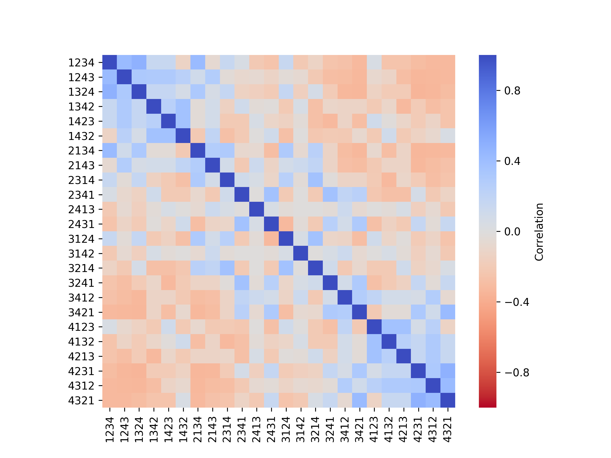
Pattern occurrences are far from independent: for example, the number of -patterns is clearly negatively correlated with the number of occurrences. Figure 1 shows the correlation of all length-4 patterns across the set of all permutations of length 8.
2.1 Permutation Classes and Structure
Permutation patterns provide a framework for analyzing the structure of permutations. The connection between patterns and block structure is most clearly seen in the case of the separable permutations, which we define here after a few preliminary definitions.
For permutations and of length and , define their direct- and skew-sum, denoted and to be -permutations as follows:
These operations are more intuitively understood graphically in terms of the plots of and . The direct sum places the plot of below and to the left of that of , while the skew sum places it above and to the left. See Figure 2.
A permutation is said to be sum- (resp., skew) indecomposable if it cannot be written as the direct (resp., skew) sum of two permutations. A decomposable permutation is one which can be written as either a direct or a skew sum in some way.
A separable permutation is one which can be decomposed as sums of the trivial permutation of length 1. For example, the permutation is separable, since
Equivalently, a separable permutation is one which is recursively decomposable: it can be decomposed into blocks which themselves can be decomposed into blocks, which themselves can be decomposed into blocks, etc. See Figure 3 for the decomposition of the plot of .
The set of separable permutations also has another important characterization: a permutation is separable if and only if it does not contain either of the patterns 2413 or 3142. Thus, a randomly chosen permutation which has this recursive block structure must have no occurrences of these two patterns. In fact, the block structure has an impact on other patterns as well. Using results from Albert, Homberger, and Pantone [2] or from Bassino, et.al. [3], we can calculate the expected number of occurrences in a random separable permutation of length . Let denote the probability that a randomly chosen 4-subset of a randomly chosen separable permutation of length forms a -pattern. Consider a random separable permutation of length , and let be the asymptotic probability that a randomly chosen -subset forms a -pattern. We have:
| (4) |
where
Recall that in the set of all permutations, all patterns are equally likely. Intuitively, this shows that a block structure within a permutation affects the number of occurrences of patterns.
2.2 Non-Overlapping Patterns
We consider a related problem: counting pattern occurrences within a single, large permutation. If we were to count all patterns, we would be counting individual entries many times: a single occurrence of the pattern 12345, for example, would lead to 5 separate occurrences of the pattern 1234. Instead, we’ll count non-overlapping patterns. Let be a permutation of length , let , and let be a family of randomly chosen disjoint subsets of , each of size 4. We consider the multiset of patterns of length 4 located at each of these sets of indices.
It follows by linearity of expectation that if is chosen uniformly at random and is any pattern of length 4, then the expected number of times that appears across the index sets is equal to . Lemma 2.1 provides a tool to simplify distribution of test statistics in later sections.
Lemma 2.1.
Suppose is a uniform random permutation of length , and let be a family of randomly chosen disjoint subsets of , each of size 4. For any , the patterns formed at indices are statistically independent.
Proof.
We can fix all of the indices outside of and permute the entries of these sets in any way. This shows that there are precisely the same number of permutations having any specified pair of patterns at . ∎
The same, however, is not true in the separable case, since permuting these entries may lead to a forbidden pattern.
For example, Figure 4 shows a uniformly randomly chosen separable permutation of length . Figure 5 shows a comparison in the non-overlapping pattern counts between this permutation and those of a permutation chosen uniformly at random from the set of all permutations of the same length.


3 Application: measuring block structure
3.1 4-permutations and Block Structure
We are given a sparse bipartite (multi)graph with edges, with total orders on the left vertices and on the right vertices.
We define a permutation of length based on the graph as follows: sort the sequence of edges according to their left endpoint, and let be the sequence of right endpoints. The values of this sequence are not necessarily distinct, but we can create a distinct sequence by introducing some small random noise: let , where is an i.i.d. sequence distributed uniformly on . Let be the standardization of .
Now, take four elements from at random, and consider their standardization.
The null hypothesis says: each of the possible outcomes is equally likely.
The alternative hypothesis says: some patterns of length 4 are more likely than others.
Here is how we propose to perform the test of versus in time, or indeed time if Steps 2 and 3 of Section 3.3 are distributed among processors.
3.2 Lehmer codes: a convenient tool
In practical computation, the ordering of right endpoints may be represented by the Lehmer code22 2 Suggested by Ryan Kaliszewski, personal communication which maps the sequence to , where
| (5) |
For example has Lehmer code . Next the mapping
| (6) |
is a bijection from to , bearing in mind that .
3.3 Four point test: computational steps
Recall that and are ordered sets of vertices, inducing two partial orders on the set of edges, namely the partial order by left endpoint, and the partial order by right endpoint, respectively.
- 0.
For tie-breaking purposes, select independently, and uniformly at random, total orders and on among the linear extensions of the partial orders induced by those on and , respectively. For example, if and are sets of integers, this can be achieved by jittering each to , where are pairs of independent Uniform random variables, for .
- 1.
Draw samples33 3 In practice, order randomly, then partition it into blocks of length four, discarding any remainder. of size four from , uniformly and without replacement. Thus no edge is sampled more than once.
- 2.
Order each block of size four, say , , by :
(7) so in if all these left vertices are distinct. Compute the standardization associated with the ordering of under , which coincides with the ordering of in , if all these right vertices are distinct. For example if the block of four is
sorting by left vertex gives
and the Lehmer code for is .
- 3.
These samples yield a vector counting the frequencies of each pattern.
Under the null hypothesis , Lemma 2.1 ensures that stores independent multinomial trials.
- 4.
- (a)
Suppose we wish to test the null hypothesis , i.e. the graph is block-free of order four, for the given orderings of left and right vertices. Perform a goodness of fit test of with respect to the multinomial distribution.
The expected value of each under the null hypothesis is . Compare the four point chi-squared statistic (4PT- for short)
(8) to the upper tail of the distribution.
- (b)
Suppose has been rejected, and we seek a scale-free measure of how much block structure the graph has, with respect to the given orderings of left and right vertices. We propose to use the total variation distance, or 4PT-TV, between the empirical probability measure which assigns mass to Lehmer code , and the uniform measure on the 24 Lehmer codes, namely
(9)
- (a)
3.4 Basic example: bipartite graph with two blocks
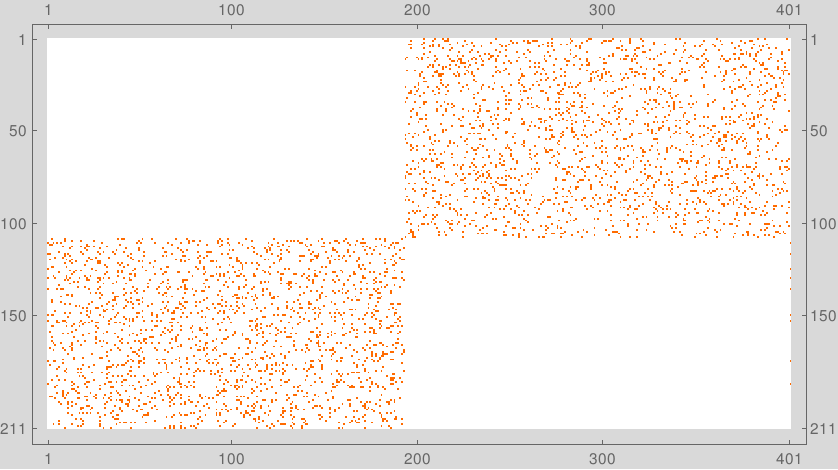
Figure 6 shows an example where all the incidences in the bipartite graph fall either in or in , for some and . Suppose proportion of incidences fall into , and proportion fall into . As in Figure 6, suppose vertices in are listed before those in , and those in are listed before those in . Call this the ordered two block model.
Suppose four incidences , , , are selected uniformly at random, labelled so that
as in (7). Let denote the number of these incidences which belong to the block. Then Binomial. For example, when , the ordering (7) implies that
Hence out of the 24 permutations, the only possible ones when are those in the set
Likewise consists of permutations where 1 is in the first place, consists of permutations where 4 is in the last place, while . From this reasoning, we obtain the simple lemma:
Lemma 3.1.
In the ordered two block model, where a proportion of incidences fall into the block, and proportion fall into the block, the relative frequency of permutation is
| (10) |
where Binomial, and is the set of permutations which are possible under the constraint that the first of belong to .
These relative frequencies are displayed in Figure 7 as a function of . This number of curves is less than 24 because there exist different choices of for which the functions coincide.

The permutations for which (the lowest value) are those in .
4 How vertex ordering affects the four point test
4.1 A pair of superficially similar but structurally different matrices
We shall set up a pair of Bernoulli matrix models, and , each with rows and columns, whose marginal statistics and likelihood ratio statistics (see Section A.3) are almost indistinguishable, but whose structure is entirely different, and then apply the four point test to each. We will also show how changing the vertex ordering of one of them dramatically changes the results of the four point test.

Figures 8 and 9 illustrate, respectively, (1) the structural difference between the two associated bipartite graphs, one of which decomposes completely into two components, like the one shown in Figure 6, and (2) the superficial similarity of their incidence matrices, under suitably randomized vertex orderings.

4.2 Bernoulli matrix model lacking block structure
Here is an elaborate pseudo-random construction based on modular arithmetic. Select positive integers and , such that are coprime. The real number has the properties
Partition the residues modulo into in any way so that
The Bernoulli parameters of are defined as follows. Fix a reference constant . Let be the residue class of modulo . Take
This deterministic scheme ensures that (to within a small discrepancy),
- 1.
There is a pseudo-random set of cells of the incidence table with parameter .
- 2.
There is a disjoint pseudo-random set of cells of the incidence table with parameter ,
- 3.
The remaining of the cells of the incidence table have parameter zero.
Furthermore the proportions of each of these three types of cell are almost the same in every row and column, thanks to the use of residue classes of modulo . Indeed every column total has mean about and every row total has mean about , since the weighted sum of the parameters in 1, 2, 3 is
The main point is that no causally sparser or denser blocks of the incidence matrix will ever appear, no matter how the rows and columns are ordered, because the placements of the zero parameters are essentially different in every row and column. A realization appears on the left in Figure 9.
4.3 Bernoulli matrix model with hidden block structure
We shall now modify the last example to produce a Bernoulli matrix model , with block structure, whose Bernoulli parameters are chosen so that the number of index pairs for which is about , the number for which is about , and the rest are zero, just as for the previous case. Recall .
Let denote a random sample of rows, and let denote a random sample of columns. The random choices of and effectively screen the block structure from visual detection, when is sufficiently small. The Bernoulli parameters of are defined as follows.
This resembles the example of Section 3.4, in that a proportion out of the expected total of incidences appear in the block, and a proportion in the block. See Figure 6. Here too every column total has mean and every row total has mean , although the variances are slightly different to those of Section 4.2. In simulations of the models 4.2 and 4.3, the resulting incidence matrices are statistically indistinguishable to the naked eye for ; see Figure 9.

4.4 Four point test applied to concrete instances
The pseudo-random model of Section 4.2, and the hidden block model of Section 4.3 were instantiated with , , and . and presented in the left and right panels of Figure 9, with 3116 and 3065 incidences, respectively. Block structure is imperceptible on the right panel, because the index sets and were selected randomly.
The four point test was applied three times to each matrix. The pseudo-random matrix scores44 4 Random sampling of 4-tuples of edges causes significant random variation in scores. were well within the -th percentile of the distribution. Similar scores were observed for the model with hidden block structure; the frequencies of different permutations are shown in Figure 10.
Finally the vertex ordering was changed for the model with hidden block structure, to make vertices in precede those in , and vertices in precede those in . Such a re-ordering could be inferred from a graph partition algorithm, such as the one55 5 FindGraphPartition [29] that produced the right pair of globs in Figure 8. Afterwards three applications of the four point test produced scores , far in the tail of the distribution, and Figure 11 shows the highly imbalanced permutation frequencies.
4.5 Practical conclusions from the case study
The case study emphasises that, when block structure is present, the four point test will reveal it only when the vertices are ordered in a way to tilt the frequencies of the permutations in . Consecutive applications of the test to the same matrix will produce answers with a statistical variability which reflects the random sampling of 4-subsets of the edges.

5 Natural vertex order computation in a bipartite graph
5.1 Choosing right and left vertex orders
We have seen in Section 4 that the ordering of left and right vertices strongly affects the output of the four point test. In this section we describe one computationally efficient method to select a natural order for the left vertices and for the right vertices, which tends to highlight block structure and to boost the Four Point Statistic. See Figure 12 for a preview. This is not the only possible method: see Section 7.3.
5.2 Symmetric linear operators
Extending the notation of Section 1.2, introduce diagonal matrices
Rescale the incidence matrix to give the matrix:
Introduce two rescaled symmetrized Laplacian operators:
| (11) |
where denotes the identity matrix. Define vectors
The following well known facts are easily checked by matrix multiplications.
Lemma 5.1.
- 1.
Both and have norm by (1), and are related by:
(12) - 2.
is a positive unnormalized eigenvector of with eigenvalue 0, i.e.
- 3.
is a positive unnormalized eigenvector of with eigenvalue 0, i.e.
5.3 Positive symmetric linear operators
We shall now shift attention away from Laplacians, towards the positive symmetric operators and . We already know that is the unique eigenvector of eigenvalue 1 for , and likewise for . Introduce a new symmetric linear operator on which composes left multiplication by with projection orthogonal to , namely
Since and , we may write this operator as a rank one perturbation of :
The corresponding operator on is
Here are some facts about them, without proof.
Lemma 5.2.
Let denote the rank of , i.e. of , and suppose the associated bipartite graph is connected. Each of the operators and has the same set of positive eigenvalues , which belong to the set . All other eigenvalues of and are zero. Moreover if denotes the eigenvector of associated with , then is an unnormalized eigenvector of associated with , and
Remark: and are known as Fiedler Vectors for the induced graphs on the left and right vertex sets, respectively.
Without loss of generality, suppose ; otherwise work instead with . Hence we put emphasis on , and derive results for from Lemma 5.2.
5.4 Power method
Proposition 5.1 (POWER METHOD).
Take a random vector whose components are independent normal random variables. Project orthogonal to , and rescale to norm 1 to obtain . Iterate for :
| (13) |
Let denote the angle such that . The event has probability 1, and in that case
| (14) |
This implies that, with probability 1, exists and is equal to or to . Provided , the convergence occurs at an exponential rate.
Proof.
This iterative scheme is the power method decribed in Golub & Van Loan [17, Theorem 8.2.1] for the computation of the eigenvector with top eigenvalue of the symmetric linear operator . The cited theorem proves the bound on . ∎
Implementation issues:
- 1.
Since an approximation suffices, we propose to fix some and to stop the iteration (13) at the first for which
For a given spectrum, (14) implies that matrix multiplies will suffice, each of which is work. We observe in practice that if the local structure of remains statistically similar as increases, the number of iterations before stopping does not vary as increases, implying that total work is . A crude upper bound for graph diameter can be obtained by selecting a left vertex uniformly at random, and taking to be twice the number of steps of breadth first search needed to cover the graph entirely. In the absence of an estimate for , we observed that in sparse graphs iterations were sufficient for convergence when . For more on the relation between graph spectrum and graph diameter, see Chung [13, Ch. 3]. The heuristic claim is that work suffices for computing an adequate natural order.
- 2.
Probabilistic arguments show that the random variable in the upper bound (14) is .
- 3.
In experiments, the ratio is typically less than , making the convergence faster than that implied by (14).
- 4.
We have phrased the iteration (13) in terms of the symmetric operator in order to appeal to the literature on the symmetric eigenvalue problem. In computational implementation the matrix is typically given by two jagged arrays, one giving a look-up by row, and the other giving a look-up by column. The iteration (13) can be implemented under the rescaling :
where is the all ones vector. The normalization step need not be performed in the norm. It can, for example, be performed in the norm instead.
5.5 Definition of natural order
Definition 5.1.
The left vertex set is in natural order if vertices are in decreasing or increasing order of the corresponding components of the eigenvector , described in Lemma 5.2. Likewise components of supply a natural order for the right vertex set .
In this definition we do not insist that or be computed precisely. Indeed an approximation, constructed as in Proposition 5.1, suffices.
See Figure 12 for an illustration of an incidence matrix transformed into natural order of left and right vertices.
5.6 Scaling behavior in natural order and four point test computations

The natural order and four point test computations have been implemented both in a Mathematica prototype and in a performant Java 10 package called QuantifyBipartiteBlockStructure.
We simulated some -regular random hypergraphs on vertices, where the vertices in hyperedge were not picked uniformly, but were a weighted sample using weight for vertex , which tends to force incidences away from the diagonal. For , we simulated two instances of such random hypergraphs for parameter choices , , . Empty columns were discarded. Figure 12 shows one of the largest matrices, both before and after the natural order computation.
The four point total variation score (9) was always in the range for the raw matrix, and in the range for the naturally ordered matrix, regardless of scale. varied as much between two matrices of the same size as it did between two matrices of different sizes. This suggests the possibility of proving limit results for values of as under suitable assumptions about the matrix generation mechanism.
The four point chi-squared statistic (8) appears to scale in proportion to in these examples. Karl Rohe [26] wrote an implementation which reveals that the significance level of the statistic is incorrect if all edges of the graph are used both (1) to derive an approximate Fiedler vector, and (2) to perform the Four Point Test. This weakness can be avoided by partitioning the edge set randomly into two subsets, one of which is used for the former, and the other for the latter.
| Review Set | # edges | # left | # right | TV | giant | TV-NO | 4PT | N.O. |
|---|---|---|---|---|---|---|---|---|
| Dig. Music | 0.836M | 0.478M | 0.266M | 0.596 | 0.703M | 0.507 | 0.484s | 7.86s |
| Android | 2.64M | 1.32M | 61.3K | 0.487 | 2.63M | 0.350 | 1.47s | 18.9s |
| Movies/TV | 4.607M | 2.089M | 0.201M | 0.418 | 4.573M | 0.321 | 2.86s | 57.8s |
| Electronics | 7.824M | 4.20M | 0.476M | 0.492 | 7.73M | 0.397 | 3.44s | 76.8s |
| Books | 22.5M | 8.03M | 2.33M | 0.308 | 22.3M | 0.349 | 14.6s | 226s |
5.7 Large natural order and four point test computations
We performed four point test and natural ordering computations on five sets of Amazon Reviews data66 6 jmcauley.ucsd.edu/data/amazon, as shown in Table 1. In all cases left vertices were reviewers, and right vertices were products of a specific type. Reading the data took longer than performing the four point test, whose time scaled linearly in the number of edges, as expected; see Figure 13. It is noteworthy that execution times for ratural ordering, which typically required about 25 iterations of the power method, also scaled linearly in the number of edges.
Only for Amazon reviews of books did the natural ordering improve the score in the four point total variation statistic (9). For the other four product categories, the original order yields a higher score. The high scores suggest that, for example, music tracks fall into music genres, and reviewers of one genre do not tend to review other genres. This effect is least for books: some reviewers may rate multiple types of literature.

6 Correspondence between permutations and bipartite graphs
The methods of this section lead to a proof of Theorem 1.1.
6.1 Random permutation generates bipartite graph: fixed vertex degrees
This section is inspired by the half-edge construction due to Wormald, and the configuration model in Bollobás [6, Section II.4]. A totally ordered left vertex set and a totally ordered right vertex set are given. Fix a left vertex degree vector , and right vertex degree vector in advance, where both vectors sum to . It is required that has degree , and has degree . It is convenient to introduce the partial sums
with , .
Construct two sequences and of vertex labels, both of length , where when , and when . Thus contains symbols referring to , then symbols referring to , and so on:
while contains symbols referring to , then symbols referring to , and so on. We call and left and right half-edge vectors, respectively.
Definition 6.1.
Given left and right half-edge vectors and , respectively, of length , the bipartite multigraph induced by a permutation is the graph whose edge set consists of the pairs
| (15) |
We estimate in Section A.6 the expected number of duplicate edges in . Blanchet & Stauffer [4] give necessary and sufficient conditions, also proved in Janson [19], for the asymptotic probability of obtaining a simple graph to be positive.
The following lemma is nearly a tautology, given the construction (15).
Lemma 6.1.
Suppose for each , and are left and right half-edge vectors of the same length , where and are the sets of distinct labels occurring in the respective vectors. Take to be bipartite (multi)graph on induced, as in (15), by a uniform random permutation . If , , and . then is asymptotically block-free.
Proof.
Fix . For any such that , select edges uniformly at random, say
where for brevity we have dropped the index from the notation. The left endpoints are already in increasing order. Since the permutation is uniformly random, the right endpoints are ordered uniformly at random. Thus the every , the sequence is asymptotically block-free of order . ∎
6.2 Inversion of the half edge construction
We shall now describe a way to invert Definition 6.1, so as to be able to produce a permutation of symbols from a bipartite graph with edges. This will be used in the proof of Theorem 1.1.
Let us elaborate on the construction of total orders on edges, introduced in Section 3.3. Fix an arbitrary total order on the edges, , with the property that, for all ,
| (16) |
In other words, the order on edges is consistent with the order on left vertices. Next generate i.i.d. Uniform random variables , which will be used as tie breakers in the following way. Extend the right half-edges above, i.e.
to a series of pairs
| (17) |
This yields another total order on the edges, namely lexicographic ordering using first the ordering on the , then the ordering on the . In other words,
| (18) |
if either , or else and .
Definition 6.2.
From the constructions above, the following Inversion Lemma is a tautology.
6.3 Permutation terminology: Property
This terminology is reproduced from [22]. Let consist of permutations on . We view each as a bijection , and we say that the length of is . For and with , let be the probability that a random -point subset of induces a permutation isomorphic to (that is, iff where consists of ). A sequence of permutations is said to have Property if their lengths tend to and for every . It is easy to see that implies .
6.4 Proof of Theorem 1.1
Take a sequence of random bipartite (multi)graphs, where , , and , which is asymptotically block-free of order 4.
Apply Definition 6.2 to convert each graph into a random permutation of symbols. From asymptotically block-freeness of order 4, and the auxiliary randomization (17), it follows that Property holds for the sequence , in the sense of Section 6.3. Theorem 1 of Král′ & Pikhurko [22] shows that Property holds for all . Together with Lemma 6.2, this implies is asymptotically block-free of order , for all , as desired.
7 Open problems
In this new area of research, many topics remain to be explored.
7.1 Directed non-bipartite graphs
7.2 Vertex exchangeability and edge exchangeability
Caron & Fox [12] present constructions of random bipartite graphs where the left vertices are exchangeable, and the right vertices are exchangeable. A general case is described by Borgs, Chayes, Cohn and Holden [10]. Cai, Campbell & Broderick [11] and Crane & Dempsey [14] have defined the notion of an edge-exchangeable graph sequence. What happens when one applies the four point test to vertex-exchangeable or edge-exchangeable graph sequences?
7.3 Minimum degree instead of natural order
The natural order defined in Section 5 is neither the only, nor the cheapest, approach to ordering rows and columns of a sparse matrix in order to expose something resembling block structure. For example, Duff et al [16] describe the minimum degree algorithm. This starts with all rows declared active, and terminates when no active rows remain. Active degree of column means the number of incidences of column with active rows. Iterate as follows:
- 1.
Select some column uniformly at random from those of minimum non-zero active degree, and place it next in the column ordering.
- 2.
Active rows incident to are placed next in the row ordering, and are then declared inactive.
- 3.
Update active degrees of columns by subtracting counts of incidences with newly inactive rows.
Column labels left over when active rows are exhausted are placed in arbitrary order, after the others. We would like to know whether applying minimum degree to some kinds of sparse matrices leads to higher or lower 4PT-TV scores than applying natural order.
7.4 Discrepancy measures in bipartite graphs
Given vertex sets and in a directed bipartite graph , let count the set of edges between and :
The total degree of vertices in , and in , respectively, is
Motivated by the notion of discrepancy, which gives one of the equivalent definitions of a quasirandom permutation [22], define the discrepancy in the bipartite graph to be the random variable
The open problem is to give computable bounds on the discrepancy of a sequence of random bipartite graphs which are asymptotically block-free in the sense of Definition 1.2. Possibly such bounds may be derived from concentration inequalities such as are found in Janson [18, Theorem 8].
7.5 Relation to quasirandom hypergraphs
Quasirandom hypergraphs are those which have the properties one would expect to find in “truly” random hypergraphs, in which a -edge contains vertices selected uniformly without replacement, and all -edges are statistically independent. Shapira & Yuster [27], Lenz and Mubayi [24], [25], and other authors cited therein, study quasirandomness in sequences of dense -uniform hypergraphs, meaning that, for some , the number of hyperedges with vertices inside any is
The study of quasirandom structures lies at the core of recent proofs of Szemerédi’s Theorem (see [5]) obtained by Gowers, and by Rödl et al. We would like to clarify how this theory of dense quasirandom hypergraphs interacts with the approach to sparse hypergraphs (viewed in terms of bipartite graphs and quasirandom permutations) that we have taken here.
Appendix A Appendix: likelihood ratio statistic for sparse binary contingency tables
A.1 Purpose
This section is intended to assuage the concerns of statisticians for whom tests of association in binary contingency table necessarily involve the likelihood ratio statistic. Koehler [23] considers the problem of testing for independence of rows and columns in a sequence of expanding two-dimensional contingency tables, where the -th table in the sequence has entries distributed among rows and columns. By contrast, traditional contingency table analysis considers a table of fixed dimensions as sample size increases; see Agresti [1].
We will see that the likelihood ratio statistic detects association between row degree and column degree in a binary contingency table, and its variance detects non-uniform incidence rates, but it does not detect block structure in sparse tables, as the Section 4 examples will show.
A.2 Likelihood ratio statistic in the Bernoulli matrix model
For simplicity consider first the Bernoulli matrix model of a binary contingency table, where incidence is Bernoulli, for some constants with values in . Let denote the set of index pairs for which . Define a log odds ratio
| (19) |
and a normalizing constant
| (20) |
The null hypothesis states that the are independent. The standardized version of the likelihood ratio statistic for testing is
| (21) |
This is an affine function of the vector of log likelihoods for the , as we see from the following elementary Lemma:
Lemma A.1.
Suppose Bernoulli() with . Take
where is the negative log likelihood, and is the Shannon entropy of . Then , and .
For convenience in normal approximation, the log likelihood is scaled so , .
Proposition A.1 (ASYMPTOTIC NORMALITY).
Consider a sequence of Bernoulli matrix models as , with Bernoulli, and index sets . Suppose the log odds ratio as in (19), divided by the normalizing constant (20), has the property that, as ,
| (22) |
Then the random variables in (21) satisfy Lindeberg’s condition:
| (23) |
Hence the rescaled likelihood ratio statistic in (21) converges in distribution to standard normal by Lindeberg’s central limit theorem.
Remark: Compare the assumption (22), where cell frequencies tend to zero, and indeed may be , with Koehler’s [23], wherein all expected cell frequencies are bounded below by a strictly positive constant as .
Proof.
The right side of (21) is a sum of independent random variables, and this sum has mean zero and variance 1. The final assertion about the central limit theorem follows from Kallenberg [21, Theorem 5.12], once we have verified Lindeberg’s condition (23).
For brevity, drop the superfix from the notation, and study a fixed . Let
Since Bernoulli, and , it follows that
Suppose is fixed. Choose sufficiently large that
For such , we have , and hence
Thus (23) is established. ∎
A.3 Examples to show log likelihood fails to detect blocks
Recall the models of Sections 4.2 and 4.3. They were designed as Bernoulli matrix models in which the Bernoulli parameters , , and 0 appear with similar frequencies, but with different structural organization. Let us study the likelihood ratio statistic for the two models.
There are two cases to consider, depending on whether the matrices and of Bernoulli parameters for the two models are known or unknown.
Parameters known: Consider the ingredients (19), (20), (21) from which the likelihood ratio statistic is derived. These ingredients are essentially the same in models of Sections 4.2 and 4.3, the only difference being in the ordering of labels, which is irrelevant when summing. Model 4.3 has block structure while model 4.2 does not. Knowledge of the parameter matrix reveals block structure, but the likelihood ratio statistic itself does not reveal block structure.
Parameters unknown: Given a pair of incidence matrices and , generated according to models 4.2 and 4.3 respectively, the statistician will observe that, for both matrices, the column totals look like samples from Binomial, while row totals look like samples from Binomial, where the unknown parameter could be estimated as or . The statistician will then compute the likelihood ratio statistic , as in (21), based on the model for all . Some cancellation occurs, and
This has mean zero, by choice of , and the question comes down to testing for excessive variance. For example, one could test whether
exceeds the quantile of , for a size test. The test results for models 4.2 and 4.3 will be similar; rejection of the hypothesis that all entries are i.i.d. Bernoulli is likely in both cases. The fact that model 4.3 has block structure, whereas model 4.2 does not, is not discovered by this test.
A.4 Regular bipartite subgraphs
The special case of a -regular bipartite graph is the one where every left vertex has degree , every right vertex has degree , and thus .
Consider a sparse case where are large, , and the set of distinct values of the and is . It makes sense to view bipartite graph as a collection of regular bipartite graphs , where consists of left vertices of degree , consists of left vertices of degree , and consists of edges with , . Thus
This is equivalent to organizing the 0-1 matrix into blocks, according to row sum and column sum. Fix a row weight and column degree . The total number of incidences in the block is as in (2). These totals may be expressed in a contingency table of the form:
A.5 Association of left and right vertex degrees
Suppose the are unknown. For a cell with , , we could estimate
| (24) |
Let count rows of weight , and let count columns of degree . Recall that counts the edges in the bipartite graph whose left endpoint has degree , right endpoint degree , as in (2). Proposition A.2 is an elementary consequence of the definitions (19), (20), (21).
Proposition A.2.
Application: Consider the null hypothesis that is a Bernoulli matrix whose parameters follows the model (24), versus the alternative that entries in cells with higher row total tend to be found in cells with higher column total. The graph theoretic interpretation of is that, for a typical edge, left degree and right degree are positively associated.
Under the likelihood ratio statistic (25) is approximately normal by Proposition A.1, but under the quantity tends to be positive when are large, which carries lower weight , but negative when are small, which carries higher weight. In any case, dependency of left degree and right degree will produce bias. Hence a two-sided test of size rejects in favor of if lies outside the range of the and quantiles of the standard normal distribution.
In summary the likelihood ratio statistic fails to detect block structure, but is capable of testing association between right and left vertex degrees in a sparse bipartite graph.
Example: Generate an incidence matrix whose rows are indexed by integers generated uniformly at random in some large window , and whose columns are indexed by rational primes exceeding . Incidence if the -th prime divides the -th integer. Discard empty rows. Only 1, 2 or 3 factors in the range are possible. If an integer has 3 factors, the largest is less than . Hence there is an association between left vertex degree (row) and right vertex degree (column).
A.6 Estimating number of repeated edges
In this section, we shall estimate the number of repeated edges for a sequence of bipartite multigraphs, constructed according to (15).
In the notation of (1), let and denote the degrees of a left vertex and a right vertex, respectively, selected uniformly at random. Their first and second moments are:
| (26) |
Denote by
| (27) |
the expected number of instances of the edge in the model (15). We may associate with any pair of count vectors as in (1) the left (resp. right) degree coefficients of variation:
and the maximum incidence rate
Proposition A.3.
Construct, according to (15), a sequence of random bipartite (multi)graphs, where , , , based upon degree sequences (1) whose left and right degree coefficients of variation converge to and , respectively, and whose maximum incidence rates converge to zero. Then the expected number of duplicate edges converges to
| (28) |
while the expected number of edges with three or more instances converges to zero.
Remark: The Poisson approximation technique used in the proof could no doubt be extended to show that the variance of the number of duplicate edges also converges to (28).
Proof.
If the number of edges were Poisson, then
and admits the same approximation. These approximations also hold for the multinomial, as we have here, when the maximum incidence rate converges to zero. Let
denote the number of edge positions which are occupied twice or more. The first moment is approximated to second order in by
in the notation of (26), which converges to (28). As for the error term,
which converges to zero. This shows that the number of edge positions which are occupied twice or more converges to (28), while the number of edges appearing three or more times converges to zero. ∎
Acknowledgments: The authors thank Michael Capalbo, John Conroy, Joseph McCloskey, Richard Lehouq, and Karl Rohe for helpful insights into the literature, and insightful comments.
References
- [1] Alan Agresti. Categorical Data Analysis, 3rd Ed., John Wiley, 2013
- [2] M. H. Albert, C. Homberger, J. Pantone. Equipopularity Classes in the Separable Permutations, Electronic Journal of Combinatorics 22 (2), 2015
- [3] F. Bassino, M. Bouvel, V. Féray, L. Gerin, A. Pierrot. The Brownian Limit of Separable Permutations
- [4] J. Blanchet & A. Stauffer. Characterizing optimal sampling of binary contingency tables via the configuration model, Random Structures & Algorithms 42, 159-184, 2013.
- [5] B. Bollobás. Modern Graph Theory, Springer Grad. Texts. Math., 1998
- [6] B. Bollobás. Random Graphs, 2nd Ed., Cambridge Univ. Press, 2001
- [7] M. Bóna. Handbook of Enumerative Combinatorics, CRC Press, 2015
- [8] Miklós Bóna. The copies of any permutation pattern are asymptotically normal. arXiv:0712.2792
- [9] Petter Brändén, Anders Claesson. Mesh patterns and the expansion of permutation statistics as sums of permutation patterns. Electron. J. Combin. 18 no. 2, 2011
- [10] C. Borgs, J. T. Chayes, H. Cohn and N. Holden. Sparse exchangeable graphs and their limits via graphon processes, arXiv 1601.07134, 2017.
- [11] Diana Cai, Trevor Campbell, Tamara Broderick. Edge-exchangeable graphs and sparsity, 30th Conf. Neural Inf. Proc. Systems (NIPS), 2016
- [12] F. Caron & E. Fox. Sparse graphs using exchangeable random measures, J. R. Statist. Soc. B 79, 1 - 44, 2017
- [13] Fan R. K. Chung. Spectral Graph Theory, American Math. Soc., 1997
- [14] Harry Crane & Walter Dempsey. Edge exchangeable models for network data, arXiv:1603.04571, 2016
- [15] R. W. R. Darling. Efficient Constructions of Heavy-tailed Random Bipartite Graphs. In preparation, 2018.
- [16] I. S. Duff, A. M. Erisman, J. K. Reid. Direct methods for sparse matrices, 2nd Ed.. Oxford UP, 2017.
- [17] Gene H. Golub & Charles F. Van Loan. Matrix Computations, 3rd Ed., Johns Hopkins University Press, 1996
- [18] Svante Janson. On concentration of probability. Contemporary Combinatorics 10, no. 3 (2002): 1-9.
- [19] Svante Janson. The probability that a random multigraph is simple. II, J. Appl. Prob. Spec. Vol 51A, 123-137, 2014
- [20] Svante Janson, Brian Nakamura, Doron Zeilberger On the asymptotic statistics of the number of occurrences of multiple permutation patterns. J. Comb. 6 no. 1-2, (2015)
- [21] Olav Kallenberg. Foundations of Modern Probability, 2nd Ed. Springer, 2002
- [22] Daniel Král′ & Oleg Pikhurko. Quasirandom permutations are characterized by 4-point densities, Geometric & Functional Analysis, Springer, ISSN 1016-443X, 2013
- [23] Kenneth J. Koehler. Goodness-of-Fit tests for log-linear models in sparse contingency tables, JASA 81, 483-583, 1986
- [24] John Lenz & Dhruv Mubayi. Eigenvalues and linear quasirandom hypergraphs, Forum of Mathematics, Sigma 3, e2, 2015.
- [25] John Lenz & Dhruv Mubayi. The poset of hypergraph quasirandomness, Random Structures and Algorithms, 46, 762-800, 2015
- [26] Karl Rohe. Personal communication. April 25, 2019.
- [27] Asaf Shapira & Raphael Yuster. The quasirandomness of hypergraph cut properties, Random Structures & Algorithms, 40, 105-131, 2012
- [28] Isabelle Stanton & Ali Pinar. Constructing and Sampling Graphs with a Prescribed Joint Degree Distribution, ACM Journal of Experimental Algorithmics, Vol. 17, No. 3, Article 3.5, 2012
- [29] Wolfram Research, Inc. Mathematica, Version 10.2, Champaign, IL, 2017