Parametric Feedback Cooling of Rigid Body Nanodumbbells in Levitated Optomechanics

Optically levitated mesoscopic particles [1] are known to be ultrasensitive detectors of force, torque, and charge [2, 3, 4, 5] and provide a range of possible applications such as detection of gravitational waves, fractional charges in bulk matter, and the Casimir torque [6, 7, 8, 9, 10]. One of the next sought-after goals in levitated optomechanics is for a nanoparticle to reach its quantum mechanical ground state. A nanoparticle in the quantum regime allows exploration of fundamental physics phenomena studying the boundary between the classical and quantum worlds, both mechanically and thermodynamically [11, 12, 13, 14, 15, 16, 17]. Other micromechanical systems in optomechanics such as microchip resonators offer similar applications [18] and have been able to attain low occupation numbers, even below $n=1$ [19, 20] due to their GHz resonance frequencies and strong coupling to light. However, these systems often require cryogenic cooling or phononic band gaps to suppress decoherence and improve quality factors since they are directly coupled to their environment [21]. Optically levitated nanoparticles are isolated from rigid structures, eliminating this source of decoherence, and can achieve quality factors $Q>10^{9}$ [22].

Much progress has been made in cooling the translational degrees of freedom (DOF) [23, 24, 25, 26, 27, 28] with a lowest reported occupation number $n=21$ [29]. Preventing further reduction in the occupation number is the efficiency with which the position can be detected [24, 25]. Shot noise on the detector from the trapping laser hinders the efficiency of position detection, and therefore decreases the effectiveness of the feedback cooling mechanism. Increasing the detection efficiency of the scattered light from the nanoparticle would allow more accurate position detection and is necessary to reach the quantum realm [30, 31].

An alternative path to the ground state and a tool for torque sensing [8, 32] is accessing control over the rotational DOF [33, 34, 35, 32, 36, 37, 38]. Whereas translational mode frequencies are typically in the kHz range, librational mode frequencies can be in the MHz range, possibly offering a more accessible ground state [3]. Cooling the nanoparticle through coupling of the translational and rotational modes has been explored both theoretically and experimentally [39, 22, 38]. Cooling of the librational modes directly has also been proposed using active feedback schemes [33]. However, these models often assume libration as the sole rotational motion. Describing the rotational dynamics in terms of libration exclusively is a good approximation for particle shapes such as nanorods because of the small moment of inertia about its symmetry axis, but this approximation will break down for particles like dumbbells with more nearly equal moments of inertia.

In this paper, we seek to investigate the intrinsic coupling between the rotational DOF by considering the classical rigid body dynamics of an optically levitated nanodumbbell with and without parametric feedback cooling. As shown below, for symmetric top-like particles, the spin of the nanoparticle about its symmetry axis, at an angular freqency of $\omega_{3}$, couples the two librational coordinates. This coupling results in two precessional modes amounting to a combination of libration and precession about the polarization axis. In the small angle limit, the equations of motion are of the same form as a charged particle in a two-dimensional harmonic oscillator plus a magnetic field. Previous investigations have dismissed the coupling that leads to precession [32, 40, 41, 42, 33, 22, 37, 43, 3], while recently, the existence of precession motion has been observed for anisotropic nanoparticles [44]. For symmetric top-like particles, $\omega_{3}$ is a conserved quantity, a feature which has important implications when considering ground state cooling of the librational motion. Surprisngly, due to the coupling of the librational coordinates, parametric feedback cooling using a linearized beam is only able to cool one of the two precessional modes. Cooling the remaining mode requires a strong frequency difference in the librational coordinates.

This paper is organized as follows. Section II introduces the classical kinetic and potential energy associated with rotations and provides a simplified model describing the motions. In Sec. III the signals of two common experimental methods to measure the orientation are calculated utilizing an incident Gaussian laser beam. Section IV investigates the effects of parametric feedback cooling with linear and elliptical polarization. Simulations of power spectral densities of the measured orientation before and after cooling are also presented. Section V addresses the effects of laser shot noise and gas collisions.

The system under consideration is a nanodumbbell optically trapped in a laser field. The particle’s center of mass is fixed at the origin so that only rotations are considered. The nanodumbbell is composed of two spheres each with mass $M_{s}$ and radius $R$. The spheres are aligned along the $z^{\prime\prime\prime}$-axis and touching at the origin, where the triple prime indicates the particle frame coordinate system (see Fig. 1). It is a symmetric top with principal moments of inertia $I_{x}=I_{y}=\frac{14}{5}M_{s}R^{2}$ and $I_{z}=\frac{4}{5}M_{s}R^{2}$. An amorphous silica nanodumbbell with mass $2M_{s}=1.029\times 10^{-17}$ kg, radius $R=85$ nm, $I_{x}=1.041\times 10^{-31}~\text{kg}\cdot\text{m}^{2}$, $I_{z}=2.974\times 10^{-32}~\text{kg}\cdot\text{m}^{2}$, index of refraction $n=1.458$, and density $\rho=2000~\text{kg}/\text{m}^{3}$ [37] is used for the calculations. The laser beam is linearly polarized along the lab frame $x$-direction and propagating in the $z$-direction with a wavelength $\lambda=1550$ nm $\gg R$, power 500 mW, and is focused by a $\text{NA}=0.45$ objective. Because the size of the nanoparticle is much smaller than the wavelength of light, the nanodumbbell is treated as a point dipole with $\vec{E}_{inc}=E_{0}\hat{x}$, the electric field polarizing the dumbbell, having no spatial dependence. Throughout this paper, the calculations are purely classical, and in what follows, exclude heating from gas collisions and photon scattering. Discussions of the effects due to heating and other noise may be found in Secs. IV and V.

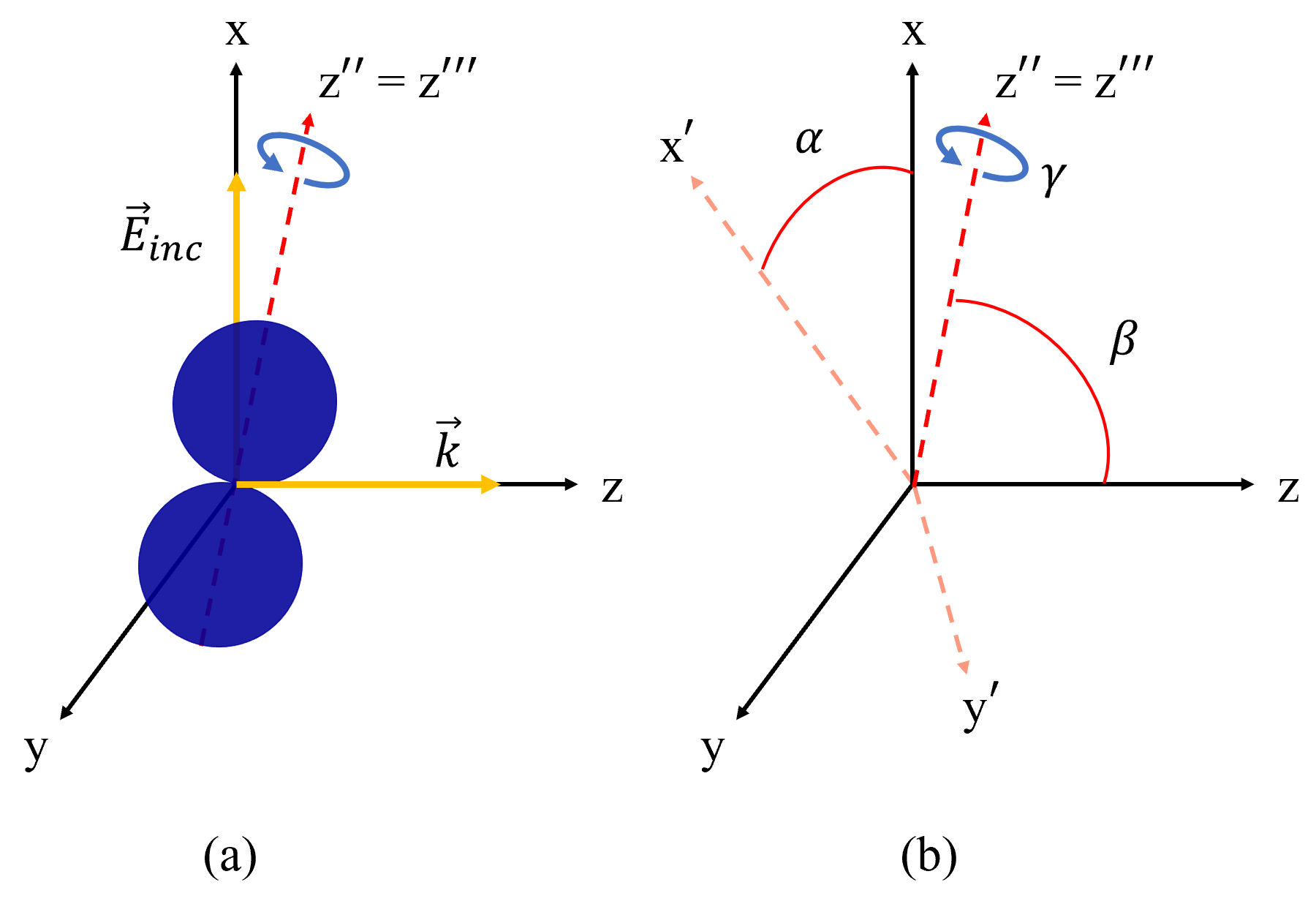
The rotational dynamics are governed by the classical equations of motion described by the Euler angles ($\alpha,\beta,\gamma$) [45, 46] in the $z$-$y^{\prime}$-$z^{\prime\prime}$ convention. To transform from the lab $(x,y,z)$ frame to the particle $(x^{\prime\prime\prime},y^{\prime\prime\prime},z^{\prime\prime\prime})$ body frame three rotation transformations are made. First, a rotation about the lab frame $z$-axis through an angle $\alpha$ is performed, $(x,y,z)\rightarrow(x^{\prime},y,^{\prime}z^{\prime}=z)$. Then, a rotation about the $y^{\prime}$-axis is made through an angle $\beta$, $(x^{\prime},y^{\prime},z^{\prime})\rightarrow(x^{\prime\prime},y^{\prime\prime}=y^{\prime},z^{\prime\prime})$. Finally, a rotation about the $z^{\prime\prime}$-axis is made through an angle $\gamma$, $(x^{\prime\prime},y^{\prime\prime},z^{\prime\prime})\rightarrow(x^{\prime\prime\prime},y^{\prime\prime\prime},z^{\prime\prime\prime}=z^{\prime\prime})$. See Appendix A for further details of the convention used in this paper.

The kinetic and potential energy are

where

is the nanodumbbell polarization vector in the lab frame and $\overset{\text{\tiny$\leftrightarrow$}}{R}$ is the rotation matrix. The $\alpha_{j}$ ($j=x,y,z$) [47, 48] are the polarizabilities for an ellipse in the particle frame ($\alpha_{x}=\alpha_{y}$) and are not to be confused with the coordinate $\alpha$. Constant terms in Eqs. (2) and (3) have been omitted as they do not affect the particle’s rotational dynamics. The $\omega_{i}$ ($i=1,2,3$) and the full equations of motion may be found in Appendix A. It should be noted that as a consequence of the nanodumbbell’s symmetry, the angular momentum about the nanoparticle’s symmetry axis, $I_{z}\omega_{3}$, is a constant of the motion. In this configuration, each Euler angle has an intuitive definition for small amplitude oscillations; $\alpha$ defines libration in the $x$-$y$ plane, $\beta$ defines libration in the $x$-$z$ plane, and $\gamma$ corresponds to angles of rotation about the $z^{\prime\prime\prime}$-axis.

The attractive potential, Eq. (2), causes the particle to oscillate about the polarization axis in two joint motions (see Fig. 2(a)). The two motions are most easily seen under a small angle approximation. It is energetically favorable for the particle’s long axis ($z^{\prime\prime\prime}$-axis) to align with the electric field and is therefore localized near the lab frame $x$-axis. This corresponds to $\alpha$ nearing towards zero or $\pi$, and $\beta$ near $\pi/2$. Allowing the two coordinates to make small oscillations about the $x$-axis, $\alpha\rightarrow 0+\xi$ , $\beta\rightarrow\frac{\pi}{2}-\eta$, with $\xi,\eta$ small, the equations of motion to first order become

where $\omega^{2}=\frac{1}{2}(\alpha_{z}-\alpha_{x})E_{0}^{2}/I_{x}$ and $\omega_{c}=\left(I_{z}/I_{x}\right)\omega_{3}$. The first term on the right hand side of Eqs. (4) and (5) amounts to libration about the polarization axis due to the trapping potential which has been seen before in [33, 40]. The second term containing $\omega_{c}$ couples the four DOF and is responsible for precession about the $x$-axis. The precession is a consequence of the non-zero angular momentum about the symmetry axis, $I_{z}\omega_{3}$. Precession has recently been seen for anisotropic particles in an elliptically polarized beam [44], but with $\alpha$ precessing around the lab frame $z$-axis with $\beta$ roughly fixed. As in the case for thin nanorods, the motion reduces to pure libration in the limit $I_{z}\rightarrow 0$. The equation of motion for $\gamma$ is not directly affected by the potential and largely evolves with time as $\gamma(t)\approx\omega_{3}t$ in the small angle approximation (see Appendix A Eq. (A12)).

The transformation of the $z^{\prime\prime\prime}$-axis into the lab frame, $\hat{r}_{z^{\prime\prime\prime}}=\overset{\text{\tiny$\leftrightarrow$}}{R}^{\dagger}\hat{z}^{\prime\prime\prime}$, determines the location of the tip in the ($x$, $y$, $z$) coordinate system,

where in the last step the small angle approximation was made. It is seen that $\xi$ and $\eta$ play the role of the $y$ and $z$ coordinates defining the location of the tip. By introducing a vector that specifies the projection of the $z^{\prime\prime\prime}$-axis on the $y$-$z$ plane, $\vec{\rho}_{z^{\prime\prime\prime}}=<0,\xi,\eta>$, it is possible to combine Eqs. (4), (5),

where $\vec{\omega}_{c}=\omega_{c}\hat{x}=\left(I_{z}/I_{x}\right)\omega_{3}\hat{x}$. The last term in Eq. (7) has the familiar form of the force on a charged particle in a magnetic field. The two joint motions now become clear as a combination of harmonic oscillations in a static pseudo-magnetic field. Thus, as long as $\omega_{c}$ is non-zero, the full dynamics of the nanoparticle must be described as a combination of libration and precession, as opposed to just libration. For a nanodumbbell at room temperature, $T=300$ K, the average value of $\omega_{c}\sim\sqrt{k_{B}TI_{z}}/I_{x}\sim 10$ kHz, where $k_{B}$ is the Boltzmann constant. While $\omega\sim 100~\text{kHz}-1~\text{MHz}\gg\omega_{c}$, the coupling that results due to the $\sim$10 kHz frequency is a resolvable feature in the power spectral density and is a non-negligible effect when considering parametric feedback cooling, as will be discussed in Sec. IV.

The librational frequency $\omega$ scales with the radius as $\omega^{2}\sim 1/R^{2}$ suggesting that a particle of smaller size is beneficial for ground state cooling. However, the polarizability and moment of inertia scale as $\alpha_{j}\sim R^{3}$, $I_{j}\sim R^{5}$ implying that the particle will be less confined and more unstable in the optical trap as the size decreases. In effect, a smaller radius will be more likely to escape the trap and will produce a broader power spectral density. Further, $\omega_{c}\sim 1/R^{5/2}$ showing that as the size of the particle decreases the precessional phenomenon is more pronounced.

Equations (4) and (5) admit two normal modes,

with $\omega_{\pm}=\frac{1}{2}\left(\Omega\pm\omega_{c}\right)$, $\Omega=\sqrt{4\omega^{2}+\omega_{c}^{2}}$, and the $A_{\pm}$, $\delta_{\pm}$ determined by initial conditions. Each mode circles the polarization axis at a particular frequency with the (+) mode advancing clockwise and the ($-$) mode counterclockwise. The superposition of the two modes results in the libration and precession mentioned above. Thus, as will be discussed in Sec. IV.3, the power spectral density of $\xi$ or $\eta$ should exhibit two peaks at $\omega_{\pm}$.

Since the coordinates $\alpha$ and $\beta$ completely describe the location of the nanodumbbell’s tip projected on the lab frame axes, it is possible to track the rotational evolution about the polarization axis while simulating the full equations of motion. Figure 2(a) plots the $z^{\prime\prime\prime}$-axis projection on the lab frame $z$-$y$ plane (i.e. $Z/2R=\cos(\beta)$, $Y/2R=\sin(\beta)\sin(\alpha)$ is plotted versus time. Note that in the small angle limit $Z/2R\approx\eta$, $Y/2R\approx\xi$). The particle’s tip undergoes fast oscillations enveloped in a slower precession motion about the $x$-axis, qualitatively consistent with the dynamics seen in the small angle approximation.

It is possible to determine the orientation of the nanoparticle with respect to $\alpha$ and $\beta$ through different types of measurements. A common method of measuring $\alpha$ libration [36, 37, 35, 38] is to first send the forward scattered light from the nanoparticle and the laser beam through a 45^∘ polarized beamsplitter (PBS). The light exits the PBS in two different directions with orthogonal polarizations. A measurement is obtained by reading the signal of each polarization state on a photodetector and taking the difference between the two signals. To determine what is measured in this procedure, consider a Gaussian laser beam incident on the dumbbell,

The Gaussian beam is defined with $\omega_{0}$ the beam waist, $\omega(z)=\omega_{0}\sqrt{1+(z/z_{R})^{2}}$ with $z_{R}=\pi\omega^{2}_{0}/\lambda$ the Rayleigh range, $\rho^{2}=x^{2}+y^{2}$, $k=2\pi/\lambda$, $R(z)=z[1+(z_{R}/z)^{2}]$, and $\psi(z)=\arctan(z/z_{R})$. The scattered light is determined by the electric and magnetic fields for a dipole in the far field [49]

where $\vec{r}$ is in the direction of observation, $c$ the speed of light, and $Z_{0}$ the impedance of free space. After exiting a collimating lens [50], the light is split by a 45^∘ PBS. The transverse components of the electric field exiting the PBS are

where $E_{x,y}$ are the $x$ and $y$ components of the total electric field following the collimating lens and $\hat{e}_{\pm}$ designate the two split polarization states after the PBS. The magnetic field undergoes a similar transformation. A measurement is performed by taking the difference between the two signals measured at their respective detectors

where $\vec{S}_{\pm}=\frac{1}{2}Re[\vec{E}_{\pm}\times\vec{H}^{*}_{\pm}]$ is the Poynting vector. Performing the integration gives a homodyne term that is proportional to the $y$-component of the polarizability from Eq. (3)

Considering that $\alpha\rightarrow 0+\xi$ and $\beta\rightarrow\frac{\pi}{2}-\eta$,

which is the angle describing the extent to which the nanoparticle’s long axis has deviated from the polarization axis in the $x$-$y$ plane. Following the same procedure above, after the collimating lens a split detection measurement is performed (which is often used to track the transverse translational motion [23, 24, 25, 26, 27, 28]) and the homodyne term is examined

which is the angle describing the extent to which the nanoparticle’s long axis has deviated from the polarization axis in the $x$-$z$ plane. Thus, both angles that will be required for parametric feedback cooling in the next section can be detected. Note that it is not possible to measure $\gamma$ directly using these methods since it is not contained within the polarization vector in Eq. (3).

Whereas the detection of translational motion relies on the $\pi/2$ Gouy phase shift from $\psi(z)$ in Eq. (10) [51], for a nanoparticle centered at the origin, the Gouy phase shift hinders detection of rotational motion. The homodyne terms in the Poynting vector evaluated far from the nanoparticle are left purely imaginary and require the imaginary part of the polarizability for orientational detection. The imaginary part of the polarizability is usually smaller than the real part [52, 48] for the types of particles used in levitated optomechanics and is two orders of magnitude smaller for a $R=85$ nm amorphous silica dumbbell in a $\lambda=1550$ nm laser field.

However, the signal may become real, and therefore larger in magnitude, if the particle is not centered at the origin, but pushed away from the focus by the laser beam in the axial direction. In Appendix B the size of the displacement in the $z$-direction is estimated by considering the radiation pressure on a nanodumbbell in the point dipole limit. Relative to the Rayleigh range, $z_{R}$, the displacement $z_{d}$ is

where $\overline{\alpha}$ is a unitless parameter defined in the polarizability as $\alpha_{0}=4\pi\epsilon_{0}R^{3}\overline{\alpha}$. For $\overline{\alpha}=0.59$, $\lambda=1550$ nm, $\text{NA}=0.45$, $R=85$ nm, $z_{d}/z_{R}\sim 0.14$. This ratio becomes important for measurements as $e^{iz_{d}/z_{R}}\sim(1+iz_{d}/z_{R})$ is a prefactor in the polarizability matrix when considering $\psi(z)$ in Eq. (10), effectively reducing the measured signal by this ratio.

Parametric feedback cooling utilizes a laser beam to trap a particle and cool its motion simultaneously through modulation of the laser power at twice the particle’s oscillation frequency [24]. To obtain a signal at twice the oscillation frequency, the coordinate to be cooled is multiplied by its time derivative $q\dot{q}$, for an arbitrary coordinate $q$.

The analyses here assume perfect and instantaneous measurements of $q\dot{q}$, which cannot be achieved in practice. Shot noise heating due to photon scattering and the effects of gas collisions are also not included to simplify the analysis. While the heating mechanisms do determine the lowest energy attainable for a fixed cooling power, the dynamical effects of gas collisions do not become important for pressures $\sim 10^{-3}$ Torr or lower and photon shot noise does not become important until the heating rate is near the cooling rate. See Sec. V for further discussion of these effects and the inclusion of noise. The results that follow thus provide a fundamental limit to cooling, irrespective of the limitations set by quantum mechanics or practical experimental parameters such as orientation detection efficiency.

It is also worth mentioning that since the equations of motion for $\gamma$ are unaffected by the trapping potential, with the dynamics determined largely by the conserved $\omega_{3}$, parametric feedback cooling only directly affects the $\alpha,\dot{\alpha}$ and $\beta,\dot{\beta}$ DOF. For this reason, the focus will be on the motions associated with $\alpha$ and $\beta$ ($\xi$ and $\eta$), as it is not possible to cool the nanoparticle’s spin about its symmetry axis using parametric feedback cooling.

The above analysis has shown that it is theoretically possible to cool the librational motion through parametric feedback cooling within a classical approximation that does not include sources of noise or heating. However, real experiments will encounter unavoidable shot noise, gas collisions, measurement uncertainty, and quantum limits.

The effects of a non-zero measurement uncertainty has been addressed in [33] showing that inefficient feedback sets a lower bound on the occupation number after cooling for a fixed cooling power. This noise source becomes important for a nanoparticle in a low occupation state $n\sim 50$ ($T\sim 1$ mK). The spin about the symmetry axis of a nanodumbbell limits the energy of the particle’s accessible DOF in the 1-100 K range after parametric feedback cooling with linear polarization (Fig. 3(c)), leaving imperfect feedback to be a negligable effect. For elliptical polarization, librational cooling is expected to be affected similarly to that found in [33] with a lower bound on the occupation number. A full quantum treatment, to be performed in the future, will test this hypothesis.

One may think it possible that gas collisions could induce an asymmetry between the librational coordinates which would allow further cooling. To test this hypothesis the effects of shot noise and gas collisions in our simulations were included for linearly polarized light. Laser shot noise was included using the methods of [33]. Gas collisions were considered as the Langevin type, $\dot{\pi_{i}}=-\Gamma_{i}\pi_{i}+\zeta(t)$, with $\pi_{i}=(\dot{\alpha}$, $\dot{\beta}$, $\dot{\gamma}$), $\Gamma_{i}=\tau_{i}/I_{i}\Omega_{i}$ the damping rate ($\Gamma_{\alpha}=\Gamma_{\beta}$) [37], and $\zeta(t)$ stochastic noise. Simulations were performed for three different pressures $P=$760, $10^{-3}$, and $10^{-7}$ Torr.

For $P=$760 Torr, the nanoparticle is unable to be cooled. The final energies conform to a Maxwell-Boltzmann distribution as it thermalizes with the surrounding gas at 300 K. Here, increasing the cooling strength $\chi$, with hope to overcome energy exchange with the gas, heats the particle as its motion is more Brownian than periodic.

For $P=10^{-3}$, and $10^{-7}$ Torr, the main results of Secs. II and IV.1 hold, with final energy distributions and PSD’s similar to that of Fig. 3(c) and Fig. 5(a), respectively. The simulations reveal that gas collisions and photon scattering do not change the general conclusions of this paper in the classical limit. The effects of laser shot noise and gas collisions while cooling using elliptically polarized light are expected to limit the lowest occupation number attainable for a fixed cooling rate and will be studied in a future report.

We have theoretically studied the rotational dynamics of an optically trapped nanodumbell with and without parametric feedback cooling. A relatively simple model describing the motions in a small angle approximation has also been provided. The nanoparticle oscillates about the polarization axis as a superposition of two modes resulting in a combination of libration and precession motions. The librational motion is due to the laser field’s potential while precession arises from the non-zero spin of the nanoparticle about its symmetry axis. The equations of motion describing the location of the tip of the nanoparticle in the small angle approximation are seen to have the same form as a charged particle in a harmonic oscillator potential and a static magnetic field.

The effect of parametric feedback cooling using a linearly polarized beam is to remove one of the two modes, resulting in pure precession. In this geometry, it is not possible to extract energy from more than two degrees of freedom and not possible to cool to the quantum regime even when information about both librational modes is available. Evidence of these dynamics may be found in the power spectral density with two peaks converging toward normal mode frequencies during the cooling process, with the smaller of the two peaks’ magnitude reducing to zero.

Using a potential energy that sets different frequencies of libration allows cooling to much lower energies when information about both librational modes are available, theoretically approaching the quantum regime in this classical analysis. The setup for cooling may be acheived experimentally by using elliptical polarization or using two perpendicular laser beams incident on the nanoparticle and feeding back both coordinate frequencies. If a single librational coordinate frequency is used in the feedback, the particle will ultimately heat. The rate of cooling is largely determined by the cooling strength and the separation between the two librational frequencies. In this case, the power spectral density will show two peaks converging toward the two normal mode frequencies with both magnitudes decreasing to zero over time.

After submission of this manuscript, Ref. [54] was published proposing a method for cooling the librational motion of an ellipsoidal nanodiamond utilizing the intrinsic magnetic dipole moment of the NV center. This method is only useful for nanodiamonds, but may have potential to cool into the quantum regime. However, Ref. [54] did not include the rotation about the symmetry axis. Therefore, it is difficult to ascertain whether the symmetry discussed in Sec. IV would be relevant. In particular, it is uncertain whether this method would allow cooling of the rotation about the symmetry axis and/or cooling of more than one librational mode.

References

- [1] N. Vamivakas, M. Bhattacharya, and P. Barker, Opt. Photon. News 27, 42 (2016).
- [2] G. Ranjit, M. Cunningham, K. Casey, and A. A. Geraci, Physical Review A 93 (2016), 10.1103/physreva.93.053801.
- [3] T. M. Hoang, Y. Ma, J. Ahn, J. Bang, F. Robicheaux, Z.-Q. Yin, and T. Li, Phys. Rev. Lett. 117, 123604 (2016).
- [4] T. J. Kippenberg and K. J. Vahala, Science 321, 1172 (2008), http://science.sciencemag.org/content/321/5893/1172.full.pdf .
- [5] D. Hempston, J. Vovrosh, M. Toroš, G. Winstone, M. Rashid, and H. Ulbricht, Applied Physics Letters 111, 133111 (2017), https://doi.org/10.1063/1.4993555 .
- [6] M. Aspelmeyer, T. J. Kippenberg, and F. Marquardt, Rev. Mod. Phys. 86, 1391 (2014).
- [7] L. P. Neukirch and A. N. Vamivakas, Contemporary Physics 56, 48 (2015), https://doi.org/10.1080/00107514.2014.969492 .
- [8] Z. Xu and T. Li, Phys. Rev. A 96, 033843 (2017).
- [9] A. Arvanitaki and A. A. Geraci, Phys. Rev. Lett. 110, 071105 (2013).
- [10] D. C. Moore, A. D. Rider, and G. Gratta, Phys. Rev. Lett. 113, 251801 (2014).
- [11] O. Romero-Isart, A. C. Pflanzer, F. Blaser, R. Kaltenbaek, N. Kiesel, M. Aspelmeyer, and J. I. Cirac, Phys. Rev. Lett. 107, 020405 (2011a).
- [12] O. Romero-Isart, A. C. Pflanzer, M. L. Juan, R. Quidant, N. Kiesel, M. Aspelmeyer, and J. I. Cirac, Phys. Rev. A 83, 013803 (2011b).
- [13] O. Romero-Isart, M. L. Juan, R. Quidant, and J. I. Cirac, New Journal of Physics 12, 033015 (2010).
- [14] Z.-q. Yin, T. Li, X. Zhang, and L. M. Duan, Phys. Rev. A 88, 033614 (2013).
- [15] J. Millen and A. Xuereb, New Journal of Physics 18, 011002 (2016).
- [16] J. Millen, T. Deesuwan, P. Barker, and J. Anders, Nature Nanotechnology 9, 425 (2014).
- [17] D. Kleckner, I. Pikovski, E. Jeffrey, L. Ament, E. Eliel, J. van den Brink, and D. Bouwmeester, New Journal of Physics 10, 095020 (2008).
- [18] P. H. Kim, C. Doolin, B. D. Hauer, A. J. R. MacDonald, M. R. Freeman, P. E. Barclay, and J. P. Davis, Applied Physics Letters 102, 053102 (2013), https://doi.org/10.1063/1.4789442 .
- [19] J. Chan, T. P. M. Alegre, A. H. Safavi-Naeini, J. T. Hill, A. Krause, S. Gröblacher, M. Aspelmeyer, and O. Painter, Nature 478, 89 (2011).
- [20] A. H. Safavi-Naeini, J. Chan, J. T. Hill, T. P. M. Alegre, A. Krause, and O. Painter, Phys. Rev. Lett. 108, 033602 (2012).
- [21] J. Gomis-Bresco, D. Navarro-Urrios, M. Oudich, S. El-Jallal, A. Griol, D. Puerto, E. Chavez, Y. Pennec, B. Djafari-Rouhani, F. Alzina, A. Martínez, and C. M. S. Torres, Nature Communications 5, 4452 (2014).
- [22] S. Liu, T. Li, and Z. qi Yin, J. Opt. Soc. Am. B 34, C8 (2017).
- [23] M. Frimmer, J. Gieseler, and L. Novotny, Phys. Rev. Lett. 117, 163601 (2016).
- [24] J. Gieseler, B. Deutsch, R. Quidant, and L. Novotny, Phys. Rev. Lett. 109, 103603 (2012).
- [25] J. Vovrosh, M. Rashid, D. Hempston, J. Bateman, M. Paternostro, and H. Ulbricht, J. Opt. Soc. Am. B 34, 1421 (2017).
- [26] T. Li, S. Kheifets, and M. G. Raizen, Nature Physics 7, 527 (2011).
- [27] P. F. B. Nathanaël P. Bullier, Antonio Pontin, “Millikelvin cooling of the center-of-mass motion of a levitated nanoparticle,” (2017).
- [28] N. Kiesel, F. Blaser, U. Delić, D. Grass, R. Kaltenbaek, and M. Aspelmeyer, Proceedings of the National Academy of Sciences 110, 14180 (2013), http://www.pnas.org/content/110/35/14180.full.pdf .
- [29] V. Jain, F. Tebbenjohanns, and L. Novotny, in Frontiers in Optics 2016 (Optical Society of America, 2016) p. FF5B.2.
- [30] V. Jain, Levitated optomechanics at the photon recoil limit, Ph.D. thesis, ETH Zurich (2017).
- [31] C. Zhong, T. Li, and F. Robicheaux, ArXiv e-prints (2017), arXiv:1708.01203 [quant-ph] .
- [32] S. Kuhn, B. A. Stickler, A. Kosloff, F. Patolsky, K. Hornberger, M. Arndt, and J. Millen, Nature Communications 8, 1670 (2017a).
- [33] C. Zhong and F. Robicheaux, Phys. Rev. A 95, 053421 (2017).
- [34] T. Li, J. Ahn, Z. Xu, and J. Bang, in Conference on Lasers and Electro-Optics (Optical Society of America, 2018) p. JF3B.3.
- [35] S. Kuhn, A. Kosloff, B. A. Stickler, F. Patolsky, K. Hornberger, M. Arndt, and J. Millen, Optica 4, 356 (2017b).
- [36] R. Reimann, M. Doderer, E. Hebestreit, R. Diehl, M. Frimmer, D. Windey, F. Tebbenjohanns, and L. Novotny, Phys. Rev. Lett. 121, 033602 (2018).
- [37] J. Ahn, Z. Xu, J. Bang, Y.-H. Deng, T. M. Hoang, Q. Han, R.-M. Ma, and T. Li, Phys. Rev. Lett. 121, 033603 (2018).
- [38] Y. Arita, M. Mazilu, and K. Dholakia, Nature Communications 4, 2374 (2013).
- [39] B. A. Stickler, S. Nimmrichter, L. Martinetz, S. Kuhn, M. Arndt, and K. Hornberger, Phys. Rev. A 94, 033818 (2016a).
- [40] B. A. Stickler, B. Papendell, S. Kuhn, J. Millen, M. Arndt, and K. Hornberger, ArXiv e-prints (2018), arXiv:1803.01778 [quant-ph] .
- [41] B. A. Stickler, B. Schrinski, and K. Hornberger, Phys. Rev. Lett. 121, 040401 (2018).
- [42] B. A. Stickler, B. Papendell, and K. Hornberger, Phys. Rev. A 94, 033828 (2016b).
- [43] C. Zhong and F. Robicheaux, Phys. Rev. A 94, 052109 (2016).
- [44] M. Rashid, M. Toroš, A. Setter, and H. Ulbricht, ArXiv e-prints (2018), arXiv:1805.08042 [quant-ph] .
- [45] J. J. Sakurai, Modern quantum mechanics, edited by S. F. Tuan (Addison-Wesley, 2011).
- [46] J. B. M. Stephen T. Thornton, Classical Dynamics of Particles and Systems, 5th Edition, edited by J. B. MARION (Cengage Learning, 2003) pp. 361 – 415.
- [47] C. F. Bohren and D. R. Huffman, “Particles small compared with the wavelength,” in Absorption and Scattering of Light by Small Particles, edited by C. F. Bohren and D. R. Huffman (Wiley-Blackwell, 2007) Chap. 5, pp. 130–157, https://onlinelibrary.wiley.com/doi/pdf/10.1002/9783527618156.ch5 .
- [48] J. Trojek, L. Chvátal, and P. Zemánek, J. Opt. Soc. Am. A 29, 1224 (2012).
- [49] J. D. Jackson, Classical electrodynamics, 3rd ed. (Wiley, New York, NY, 1999).
- [50] L. Novotny and B. Hecht, Principles of Nano-Optics (Cambridge University Press, 2006).
- [51] A. T. M. A. Rahman, A. C. Frangeskou, P. F. Barker, and G. W. Morley, Review of Scientific Instruments 89, 023109 (2018), https://doi.org/10.1063/1.5008396 .
- [52] K. Dholakia and P. Zemánek, Rev. Mod. Phys. 82, 1767 (2010).
- [53] W. H. Press, S. A. Teukolsky, W. T. Vetterling, and B. P. Flannery, Numerical Recipes 3rd Edition: The Art of Scientific Computing, 3rd ed. (Cambridge University Press, New York, NY, USA, 2007).
- [54] L. Ge and N. Zhao, Phys. Rev. A 98, 043415 (2018).