Dynamical structure factor in the non-Abelian phase of the Kitaev honeycomb model in the presence of quenched disorder
Abstract
Kitaev’s model of spins interacting on a honeycomb lattice describes a quantum spin-liquid, where an emergent static gauge field is coupled to Majorana fermions. In the presence of an external magnetic field and for a range of interaction strengths, the system behaves as a gapped, non-Abelian quantum spin-liquid. In this phase, the vortex excitations of the emergent gauge field have Majorana zero modes bound to them. Motivated by recent experimental progress in measuring and characterizing real materials that could exhibit spin-liquid behavior, we analytically calculate the dynamical spin structure factor in the non-Abelian phase of the Kitaev’s honeycomb model. In particular, we treat the case of quenched disorder in the vortex configurations. Our calculations reveal a peak in the low-energy dynamical structure factor that is a signature of the spin-liquid behavior. We map the effective Hamiltonian to that of a chiral p-wave superconductor by using the Jordan-Wigner transformation. Subsequently, we analytically calculate the wave functions of the Majorana zero modes, the energy splitting for finite separation of the vortices and finally, the dynamical structure factor in presence of quenched disorder.
I Introduction
Quantum information processing using creation and manipulation of topological excitations in low-dimensional systems have been the focus of intense investigations lately. These topological excitations can be used to encode logical information in the form of qubits. These topological qubits have robust coherence properties since they are immune to noise arising from local perturbations Kitaev2003; Kitaev2006; Nayak2008; Terhal2015. One of the most promising candidates for topological qubits is using Majorana zero modes (MZM-s) Kitaev2001; Terhal2012; Landau2016; Roy20172. Four MZM-s can be used to encode a qubit Bravyi2006. The non-Abelian braiding statistics of the MZM-s, together with magic state distillation, can be used to perform all the single and two-qubit gates required for universal quantum computing Bravyi2005; Kitaev2006; Bravyi2006; Leijnse2012. There are several proposals to experimentally realize these MZM-s Fu2008; Alicea2010; Akhmerov2011. One of the most promising directions is to realize experimentally Kitaev’s toy model of a 1D, spinless, p-wave superconductor Kitaev2001. Recently, remarkable progress has been made in experimental realizations of this model Delft2012; Copenhagen2016; Delft2017. Alternately, MZM-s were already proposed to exist in 2D chiral p-wave superconductors Read2000; Alicea2012.
This work concerns the MZM-s that were predicted to arise in Kitaev’s exactly solvable honeycomb model Kitaev2006. The model describes spins interacting on a honeycomb lattice, where the nature of the interaction depends on the direction of the link on the lattice. Due to the interaction, the spin degrees of freedom fractionalize into Majorana fermions, interacting with an emergent static gauge field Senthil2000. Depending on the choice of the interaction strength, the system is either in a gapped, toric code phase with Abelian anyons or in a gapless phase. Addition of an external magnetic field while being in the gapless phase opens a gap in the spectrum Kitaev2006; Burnell2011. It is then that vortex defects of the static gauge field trap MZM-s, which have the desired non-Abelian exchange statistics and can, in principle, be used for quantum information processing. As will be shown below, the model in this phase can be mapped to the chiral p-wave superconductor which then naturally gives rise to the MZM-s Burnell2011; Roy2017; Hur2017.
Apart from hosting MZM-s that are generally interesting for the purpose of quantum computing, the honeycomb model describes a quantum spin liquid (QSL). The latter is a phase of matter that is highly frustrated and has no ordered ground state even at zero temperature. In the last decade, there has been a lot of theoretical and experimental effort to characterize different materials with interactions similar to that of Kitaev’s honeycomb model and finding a QSL phase of matter (Lee2008; Jackeli2009; Leon2010; Witczak-Krempa2014; Rau2014; Winter2017; Zhou2017; Savary2017; Hermanns2018; Ducatman2018; Hickey2018). There is experimental evidence that certain materials, among them for example -RuCl3, are dominated by the interaction of the Kitaev honeycomb model Khaliullin2005; Jackeli2009; Plumb2014. These materials show QSL behavior above certain temperatures. However, if cooled sufficiently, all these candidates tend to magnetically order due to additional non-Kitaev interactions. Recently, an NMR measurement of H3LiIr2O3 showed no sign of magnetic ordering at all (Kitagawa2018) while a large set of low energy states was observed in the specific heat and the NMR measurement results. This indicates spin liquid behavior in H3LiIr2O3 that still lacks a good model describing the findings. As a reaction to this experiment, different proposals are under discussion to explain the results(Slagel2018; Kimchi2018; Knolle2018). One promising approach is to consider disorder in the model’s interaction strengths, analyzing the “bond-disordered Kitaev model” (Knolle2018).
In this work, we treat a different problem where we analyze the non-Abelian phase of Kitaev’s honeycomb model in the presence of quenched disorder of vortex configurations. Since the gauge field and its vortices are static quantities in Kitaev’s model, we expect this situation to be well-described by an average over quenched disordered configuration of vortices. To characterize such a system, the dynamical structure factor is indispensable, which can potentially be measured with neutron scattering. We provide analytic results of the low energy dynamical spin structure factor. We find that in the presence of vortices, the dynamical structure factor has an additional peak centered at the energy (also called the flux gap, which is the energy added by an excitation of the gauge field due to the presence of two additional vortices) with an unusual decay behavior proportional to , where is the frequency and defines a scale that depends on the applied magnetic field strength. This peak and the decay is a signature of the vortices present in the sample. Moreover, we provide analytical results for the energy-splitting due to hybridization of MZM-s and the wave functions, which agree well with previous numerical findingsNussinov2008; Cheng2009; Lahtinen2011; Knolle2014; Knolle2014; Gohlke2017.
The paper is organized as follows. In Sec. II, we describe Kitaev’s honeycomb model in a magnetic field in terms of Majorana fermions by using a Jordan-Wigner transformation. Subsequently, we provide a continuum description of the system. In Sec. III, we calculate the wave functions of the MZM-s in the continuum model. In Sec. IV, we present results for the splitting of the ground state energy due to a finite overlap of the wave function of two MZM-s. In Sec. V, we calculate the low energy contribution to the dynamical structure factor in presence of two vortices. Finally, in Sec. VI we consider a quenched disordered distribution of vortices and calculate the dynamical structure factor. In Sec VII., we summarize our findings.
II Description of the Model Hamiltonian

We consider spins on a honeycomb lattice, in the presence of an external magnetic field. The total system Hamiltonian is given by . The lattice consists of two sublattices as indicated by the black and white sites in Fig. 1. Every site is labeled by the index , where label the position of a z-link [see the labels of the links in Fig. 1 (a)] while or indicates if the site sits on the black or the white sublattice. The Hamiltonian reads
| (1) |
where the sum over x-links runs over contributions where and are connected by a link with label x in Fig. 1 (a) (and equivalent for y and z). At this point, the arrows in the figure are irrelevant, but they will be important further below. In the absence of a magnetic field, the system can either be in a phase with a gapped spectrum or in a phase with gapless spectrum, depending on the choice of couplings. Following Ref. [Kitaev2006], we analyze the system at its isotropic point that corresponds to the gapless phase. Applying an additional magnetic field to the system breaks the time-reversal invariance. This perturbation opens a gap in the spectrum and then, the vortex excitations trap MZM-s. The additional contribution to the Hamiltonian due to the magnetic field is given by
| (2) |
with . The sum over denotes a sum over three neighboring sites for which we have to satisfy the following rules when assigning to the sites. To understand these rules, note that the three neighboring sites partly encircle a plaquette as shown in Fig. 1(a). The label and thus the operator always belongs to the site that has an x-link pointing away from this partly encircled plaquette. The same applies for the operator with a y-link and the operator with a z-link. An example configuration is shown in Fig. 1(a). Next, we show how the Hamiltonian of the system can be mapped onto that of non-interacting fermions. To this end, we use the Jordan-Wigner transformNussinov2008
| (3) | ||||
| (4) |
where the product symbol denotes a product over all sites along the Jordan-Wigner string (JWS) from its beginning to , along the path shown in Fig. 2. Moreover, we introduce the Majorana operators

| (5) |
The original spin Hamiltonian maps to a Hamiltonian that is quadratic in the Majorana operators with only nearest neighbor interactions. In addition, the magnetic perturbation provides a coupling between next-to-nearest neighbors. The Hamiltonians are given by
| (6) |
where the terms in are identical to the terms in Eq. (II) with the important difference that the direction of the arrows in Fig. 1 (b) are now relevant as it defines the ordering of the product of Majorana operators. In particular, the operator has to be to the right of if there is an arrow starting at the site and terminating at . The terms in comprise the next to nearest neighbor links labeled by x⟂, y⟂ and z⟂ (perpendicular to the original links) as shown in Fig. 1 (b). Note that all hopping terms are among the -Majoranas while the -Majoranas only appear in form of the ; here denotes a site on the white, on the black sub-lattice, and labels the z-link at position between the sites and . Every term in Eq. (II) that has a vertical component along a z-link is multiplied by the of the corresponding link. Since , all -s have eigenvalues . Furthermore, all -s commute with the Hamiltonian and, thus, they are conserved. Denoting the plaquette by the index of the vertical link to the left of the plaquette, we find that for each plaquette, there is a conserved quantity with eigenvalues . If , the plaquette carries a vortex, which is an excitation of the gauge field. Since the -s are conserved, it follows that the gauge field has no dynamics Kitaev2006; Gohlke2017. The position and number of vortices are the physical properties that define the sector of the Hamiltonian when choosing the configuration of the gauge field 11 1 Note that in the original Kitaev paper Kitaev2006 a degree of freedom was attached to ever link. In our model, only the z-links have this gauge degree. The reason is that using the Jordan-Wigner transform contains already a choice of gauge that is equivalent to choosing the gauge field along the x- and y-links to be 1.. All choices that do not change these properties are gauge equivalent(Kitaev2006; Alicea2012). It turns out that each vortex hosts a localized MZM. In the following, we quantify the spatial distribution of these zero modes and their physical implications.
First, we embed the system into real space by choosing a unit-cell as shown in Fig. 1 (c) with vectors and and the lattice constant . The position of the black site in each unit cells is given by the vector . The ground state of the system is vortex free Kitaev2006. The simplest choice of gauge for the vortex free sector is to choose for all . Since this choice is translation invariant, we analyze the resulting Hamiltonian in Fourier space. The Hamiltonian is given by
| (7) |
with
| (8) |
where is the total number of unit-cells and the length of the system. The matrix elements read
| (9) |
The off-diagonal elements in the Hamiltonian originate from while the diagonal elements are due to the magnetic field. The function vanishes at the Dirac points . Close to these points the spectrum is linear. Expanding around leads to .
The magnetic contribution to the Hamiltonian gives rise to a gap in the spectrum of size . As we are interested in the low energy properties of the system, we linearize the Hamiltonian in the vicinity of the Dirac points and apply a continuum approximation. For this purpose we introduce the new complex field operators . The new fermions satisfy the relation (valid in the limit )
where the factor is the square root of the area of the unit cell. The vector without the subscript indicates that it describes a point in the continuum instead of the lattice sites . In this picture, the annihilation operator corresponds to the contribution of the Dirac cone at while the creation operator corresponds to the opposite Dirac cone at . The new operators obey the canonical fermionic relations
| (11) |
In the following, we make use of a 4D Bogoliubov-de Gennes representation and introduce the spinor . The first two entries contain the hole (annihilation) operators and the last two entries the particle (creation) operators 22 2 Note that in our case particles correspond to the first Dirac point while holes correspond to the other Dirac point. Note that the operator obeys the symmetry
| (12) |
here swaps the / degrees of freedom while the matrix acts on the particle-hole degrees of freedom. In the continuum limit, the Hamiltonian reads

| (13) |
with the Bogoliubov-de Gennes Hamiltonian
| (14) |
here, we have introduced the velocity
of the Majorana modes. The Hamiltonian in Eq. (14) is block diagonal in the particle-hole degrees of freedom33 3 Note, that in the upper block the spin-up like state corresponds to a Majorana operator attached to a white site in the lattice and the spin-down like state to a Majorana operator corresponding to a black site, while in the lower block this choice is reversed., which is expressed by the identity operator . This property originates from the fact that we ignored fast oscillating terms proportional to .
III Calculation of the zero-mode wave function
The aim of this section is to derive an analytical expression for the wave function of the bound zero modes of a sufficiently isolated vortex. The vortex is described by setting all except for the on the z-bonds along a horizontal line that starts at the vortex position and ends at infinity as shown in Fig. 3. This can be expressed as a Hamiltonian describing a system with a single vortex. The potential term adds a vortex to at the origin. As the system obeys translation invariance, the resulting zero mode is general and can later be shifted to any position in the sample. In the continuum approximation, the potential changes only along a horizontal line and can be implemented by changing the boundary conditions of the solution along this line: in particular, we require the wave function to change sign when crossing the line. Further below, we show that this line manifests itself as a branch cut.
For the calculation of the zero mode, we need to solve the equation
| (15) |
The Hamiltonain is block diagonal in the space of the two Dirac cones and can be solved separately for each block. Thus, the problem reduces to solving the equation
| (16) |
where we have introduced , which will turn out to be the inverse decay length of the zero mode. Due to the radial symmetry, it is simpler to solve this problem in polar coordinates. Transforming Eq. (16) yields
| (17) |
where is the angle with respect to the positive -axis. This choice implements a branch cut on the positive -axis so that the ansatz
| (18) |
with satisfies the boundary conditions and changes sign when crossing the branch cut. Inserting the ansatz into Eq. (17) leads to the two equations
| (19) |
The first equation tells us, that the zero mode is radial symmetric. From the second equation, we find the explicit radial wave function
| (20) |
Note that our result is qualitatively different from the wave function that would describe the MZM in a chiral p-wave superconductor Read2000; Alicea2012 even though after Jordan-Wigner transform, both Hamiltonians are the same modulo irrelevant constants. The wave function in the case of a p-wave superconductor with the same Hamiltonian has only an exponential decay without the power-law dependence. The difference is due to the fact that in the superconducting case, one searches for a solution which is periodic in and thus, half-integer -s. This leads to an edge mode around the defect which is not at zero energy. The zero-mode then arises by introducing a half-a-flux quantum magnetic vortex in the defect, which then give rise to a zero-energy mode. In the case of the honeycomb model, the vortex defect of the gauge field is sufficient to give rise to the zero energy mode by itself. The key point here is that the charge degree of freedom of electrons couples to electromagnetic fields. This gives rise to qualitatively different physics compared to that arising from interacting spins, even though the Hamiltonians in the two cases appear to be similar.
The lower block of Eq. (15), corresponding to the opposite Dirac cone, has the same solution for the wave function. To satisfy the symmetry, Eq. (12), of the spinor the full zero mode has to combine both Dirac points. Additionally, we require the absolute value of the black and white components of the wave function to be continuous when passing through the vortex along the line of the branch cut. Using these criteria leads to the normalized spinor for a zero mode bound to a vortex at the origin, reading
| (21) |
where . The wave function decays exponentially due to the decay length introduced by the magnetic field in addition to an algebraic decay . The latter corresponds to the conventional decay of a radial symmetric wave.
From Eq. (II), we can read off the transformation behavior of the wave function when we shift the Hamiltonian by a vector , representing the position of a vortex not at the origin. The hole components are multiplied by a phase factor , while the particle components need to be multiplied by . This leads to the general MZM wave function bound to a vortex at position given by
| (22) |
where is the angle defined with respect to an axis parallel to the -axis that runs through the vortex core at . From this we find the zero mode operator
| (23) |
with and . Note that is manifestly Hermitian and therefore, represents a MZM. In Fig. 4 we compare the numerical exact wave function, obtained by numerically diagonalizing Eq. (II), to our analytic expression. The agreement is rather good even for moderate distances from the vortex core.
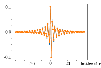
IV Computation of the energy splitting in the presence of two vortices

Above, we calculated the wave function of the zero mode bound to a single vortex in the Kitaev honeycomb model. If there are two vortices, each of these carries a zero mode. Provided that the vortices are separated sufficiently, this leads to a two-fold degenerate ground state. However, if the vortices approach each other, the zero modes hybridize to give rise to a conventional fermionic mode and, as a result, the ground state is no longer degenerate. The aim of this section is to calculate the energy difference between the ground state and the first excited state that arises due the hybridization between two MZM-s.
We split the Hamiltonian , describing the system and the two vortices, into the Hamiltonian for a system without vortices and the two potential terms and , which each add a vortex. We project the eigenvalue equation into the low energy sub-space of the two zero modes. To second order, the energy splitting is given by
| (24) |
where are the MZM wave functions for a vortex at position as given by Eq. (22). Our main task is to determine the matrix element . For the evaluation of the latter we can use the fact that we are dealing with zero modes with the properties and conclude
| (25) |
In Sec. III, we implemented the potential that adds a vortex by changing the boundary condition of the unperturbed system for the wave function. However, here it is more convenient to have an explicit expression for the vortex potentials and . The potentials needs to switch the sign for all hopping interactions along the branch cut of the corresponding vortex. For the calculation of the energy splitting, we introduce the geometry as shown in Fig. 5. We choose the branch cut of the vortex further right on the -axis to point to positive infinity. Thus the angle around the vortex with respect to an axis that runs through the vortex parallel to the -axis is defined as . For the vortex further left on the -axis, we choose the branch cut to point in the opposite direction so that the angle with respect to an axis that runs through this vortex parallel to the -axis is defined as . This choice keeps the two potentials locally separated and avoids that and have terms in common. A simple way to find the explicit form of the potentials and is to consider twice the negative -interaction terms along the branch cut of the second quantized Hamiltonian. By applying the continuum approximation and using the Bogoliubov-de Gennes representation to
| (26) |
we can read of the potential . Here we defined as the set of z-links on the branch cut that belongs to the vortex with branch cut 1. The potential assumes the form
| (27) |
where we ignored the fast oscillating terms . Here, is the -component and the -component of the vortex position . In this continuum approximation, the potential has finite weight only on the branch cut, which is ensured by the -function in -direction and the -distribution in -direction. The -distribution is multiplied by a factor of , which is the width of the unit-cell in -direction. By acting with the potential on the wave function of the MZM, it adds a minus sign to the black components of the wave function, while leaving the white components untouched. This implements the desired sign change of the wave function across the branch cut, as the white components sit above while the black components sit below the branch cut.
Proceeding similarly, we can obtain the potential . However, for the following calculation we choose to evaluate the matrix element , which contributes only on the branch cut 1 (see Fig. 5). This leads to the ambiguity that both, the choice and , represent the wave function on the branch cut. However, if we consider the real lattice, we need to take into account again that sites on the black sub-lattice always sit below the branch cut while sites on the white sub-lattice always sit above the branch cut. To implement this fact in the continuum model, we have to set for the spinor components of the white sub-lattice and for the spinor components of the black sub-lattice. Evaluating the matrix element, we find
| (28) |
where . This term has a direction dependence by the factor that implements the properties of the honeycomb lattice in the continuum model. Beyond that, we expect the splitting to be isotropic because we treat the isotropic Kitaev model. Therefore, the result of the integral needs to be independent of the angle . We checked analytically that the integral, except of the factor , indeed does not depend on the angle , as long as the distance between the vortices is fixed. Thus, we can choose for simplicity and define to find
| (29) |
where we assumed large distances between the vortices with and replaced , valid in regions where the integrand has relevant contributions. With this, the energy splitting reads
| (30) |
The splitting has the same decay properties as the Majorana wave functions. The only angular dependency comes in by the sixfold symmetric factor . Note that there are no vortex positions on the lattice where the prefactor is exactly zero. However, for large distances between the vortices almost any vector can be approximated and the splitting oscillates depending on the direction of of the vortex separation.
V Calculation of the dynamical spin-spin structure factor
In Sec. III and Sec. IV, we have calculated the MZM wave functions and the splitting of the ground state energy due to finite overlap of two such MZM-s. In this section, we treat the case of a large number () of MZM-s and analytically calculate the dynamical structure factor for energies below the gap using the energy splitting and MZM wave functions obtained above. We consider the case where the temperature is below the gap with but still large compared to the scale of the average hybridization splitting of two Majorana modes with [see Eq. (30)], where is the typical distance between vortices. In this limit the system is in an equal mix of the almost-degenerate ground states. This low energy eigenspace is spanned by the states , satisfying with energies . Here, is a number, where each bit represents the occupation of an eigenmode in the low energy space. The structure factor is then given by
| (31) |
where and reads
| (32) |
Here are the Pauli matrices in the Heisenberg picture. The spin-spin correlation in the Kitaev honeycomb model is ultra short ranged and only nearest neighbor and on-site correlators that correlate spins from the same type, i.e. , add finite contributions Kitaev2006; Tikhonov2011; Knolle2015. Therefore, we have only if or if and represent nearest neighbors. As we are working with the isotropic model (), the structure factor is the same for all three types of interactions and directions. Therefore, we only calculate the -structure factor and suppress the interaction labels from now on. For the -structure factor, only sites separated by a z-link and on-site terms contribute to Eq. (V). Thus, we can replace for the z-link contribution and for the on-site contribution resulting in
| (33) |
where is the y-component of the momentum vector . Applying the Jordan-Wigner transformation leads to the expression
| (34) |
if and
| (35) |
if . In these expressions, the operators are the Majorana operators introduced in Sec. II. The Hamiltonian that appears in the time evolution of the transformed matrix elements is the Hamiltonian with two additional vortices in the plaquettes directly adjacent to the link between sites and Knolle2015. It satisfies the equation with eigenmodes and energy . The label represents a bit string like the label , with , where each bit represents the occupation of a mode. The energy of the mode hosted by the two extra vortices in is close to the energy of the gap, because the vortices are separated only by one plaquette and thus the energy splitting is maximal. Therefore, the extra vortices are not relevant for the low energy structure factor, except for an energy shift that is caused by the raise in excitations of the gauge field from to vortices. This energy shift is called the flux gap , which is the difference in the ground state energies of the Hamiltonian and (at the isotropic point , see Ref. Kitaev2006).
It is useful to write down the Lehman representation of the dynamical structure factor reading (for , otherwise it is multiplied by )
| (36) |
We assume a dilute gas of vortices with a low vortex density satisfying . This implies that for the creation of a fermionic eigenmode it is a good approximation to take only two MZM-s localized close to each other into account. The operators that create single eigenmodes are given by the superposition of two MZM-s and bound to vortices at position and with . The pairing of the zero modes and has to be done in a way that the sum of the distance between all chosen pairs of vortices in the sample is minimized. The choice of the plus or minus sign has to be taken so that the operator annihilates the ground state , which depends in general on the sign of the energy splitting in Eq. (30) without the absolute value. Note that the final structure factor will not depend on these signs. The subgap states are thus given by , where is the th bit of . As the creation and annihilation operators and are localized objects, they do not differ significantly for and , especially as differs only locally from , too. Therefore we can assume that the eigenstates of are created by the same operators as the one for with , where is the th bit of .
Only matrix elements between states and that differ in the occupation of a single bound mode have a finite contribution to Eq. (V). This stems from the fact that the Majorana operators change the fermion parity by one. In other words, only matrix elements labeled by and that differ by a single bit contribute. Labeling the position of this bit by , one of the sums over and in Eq. (V) can be reduce to a sum over . The other sum results in a simple multiplication by the prefactor , because there are different states that differ by the same single bit of and . All these states add the same contribution to Eq. (V). This leads to
| (37) |
where is the energy of mode and is a single mode term that we introduce as
| (38) |
For the calculation of this term, it is convenient to apply the continuum approximation, so that we can use the Majorana operators from Eq. (III) to express the fermionic modes . By additionally expressing the Majorana operators with Eq. (II) by the Dirac fermions , we can proceed with the calculation by using the canonical commutation relations between the Dirac fermions. If we first take only the on-site contributions into account, we find in the continuum approximation
| (39) |
where the continuous vector points to the position of the unit cell containing the site . In the continuum approximation, the label is kept only for the purpose of indicating that represents the on-site contribution. The function is the decaying prefactor of the spinor given in Eq. (22) and is the overlap between the vacua of the different flux sectors with approximately at the isotropic point of the Kitaev honeycomb model Knolle2015. The angles and are the angles corresponding to the vortices, which are defined with respect to an axis that runs through the vortex parallel to the -axis as shown in Fig. 5. The on-site contribution consists of terms that depend only on the wave function of a single MZM. In contrast, the nearest neighbor contribution to the dynamical structure factor is complex with imaginary and real part
| (40) |
As for the on-site contribution, the label is kept only to indicate that it is an off-site contribution, while the vector describes the position of the unit cell containing the sites and . The real part of the structure factor is diagonal in the wave functions and contains only single MZM terms. The imaginary part is off-diagonal and proportional to the overlap between the wave functions of the two MZM-s that from the complex fermionic eigenmode. Inserting these results into Eq. (V) and using that , the dynamical structure factor reads
| (41) |
The formulas given by Eq. (39) and Eq. (V), together with Eq. (V), provide, up to spatial integration, an analytic expression for the sub-gap dynamical structure factor . In frequency space, it consists of isolated -peaks distributed around the flux gap energy , because this is the energy that needs to be excited to switch the flux sectors from vortices to vortices. The exact position of these peaks in frequency space depends on the distribution of vortices and their distances to each other. In real systems however, the vortices will be distributed randomly. Therefore, we consider a quenched disorder average of the structure factor over the positions of the vortices in the next section.
VI Structure factor in the presence of quenched disorder
We consider vortices which we divide into pairs (), where and point to the vortex positions. The reason for this notation is explained below. We assume the positions of the vortices in the sample to be distributed randomly and thus apply a quenched disorder average over these positions. We treat these as random variables without dynamics caused by the Hamiltonian of the system. The average structure factor reads
| (42) |
where is the probability that a given vortex configuration is realized. Such a quenched disorder average smears out the -peaks and introduces a natural broadening that we quantify in the following.
As the fermionic eigenmodes in the sub gap region depend on the distance between the vortices, we need to pair up the correct vortex bound states depending on the configuration . With the vortex density so low that at most two vortices are close to each other, we can approximately minimize the sum of the distances between all chosen pairs by pairing up a vortex at position with its closest neighbor at to form the eigenmodes . This implies that the distribution factorizes with , where is a two-body probability distribution. It is defined by
| (43) |
and returns the probability of having a vortex at an arbitrary position with its closest neighbor at distance from the point . It is normalized to . The typical vortex spacing can be expressed by and is thus large for small vortex densities. We assume the latter to be so small that , which assures that our assumption to take only two vortices close to each other into account is consistent. We checked numerically that Eq. (43) corresponds indeed to the correct distribution of finding the closest point to another point in a 2D sample of randomly but uniformly distributed points.
Each term in Eq. (V) depends only on two vortex positions. Thus, we need to perform only two 2D non-trivial integrals. After averaging, each eigenmode labeled by in Eq. (V) adds the same value to the final result, so that solving only one of the two-body integrals explicitly is sufficient. Therefore, we use for all expressions in the following. As the average distance between the vortices proportional to is large compared to the lattice constant, we are interested in the structure factor at small . Due to the ultra short ranged correlators, there is only little structure in -space Knolle2015 and therefore we restrict our calculations on for simplicity. Evaluated at , the structure factor can be measured in electron spin resonance. Its leading contribution is given by the on-site term because is not relevant at due the prefactor and is always sub dominant. The latter stems from the fact that the factor is always exponentially smaller than one of the diagonal terms or . It remains to solve the integral
| (44) |
As appears only in differences with the vortex positions , the final result will be independent of the correlators position and thus we set for each integral. It is useful to introduce the relative vortex distance and a center of mass coordinate . The -distributions as well as the probability density are independent of the center of mass coordinate. Therefore, it is best to perform the center of mass integral first. The second term in the on-site contribution of Eq. (39) proportional to oscillates fast on the scale for the center of mass integral while changes only slowly. Therefore, the oscillating term averages out and only the isotropic44 4 In this case, isotropic means modulo the directional dependence of the energy splitting first term in Eq. (39) remains. Note that if there are no oscillations that can average out the contribution. However, this is only relevant for a single direction in a 2D system and thus the contribution to the final result is still small. Inserting the wave functions, the remaining integral in relative and center of mass coordinates reads
| (45) |
In the second step, we performed the center of mass integral which is independent of the -distributions and the probability density . In the remaining integral, the -distributions contribute for vortex separations that satisfy . From this, we find the angle integral from in the continuum limit to result in the factor
| (46) |
where the radial symmetric is the energy splitting between vortices without the direction depended oscillations, see Appendix A. The remaining integral
| (47) |
can be solved numerically and leads to a peak in the dynamical structure factor at , see Fig. 6. This peak is the signature of the zero modes inducing the -fold degenerate ground state.
To provide analytical results describing the peak, we note that the factor introduces a cutoff at
| (48) |
which is the approximate solution of the equation valid for with
| (49) |
The height of the peak can easily be found by evaluating Eq. (47) at . We find
| (50) |
with being the Gamma function. To find an analytic expression for the shoulder of the peak and its decay behavior we use that for the decay the integrand is dominated at . We expand the factor under the square root in around up to first order and replace the remaining variables by the dominating . Here, we find
| (51) |
The results show that the shoulder of the peak has an unusual decay proportional to . This interesting feature and the position of the peak centered around are signatures for the presence of MZM-s in the system. We compare the analytic results to the numerical results in Fig. 6.
The decay of the structure factor depends on the five important parameters and . The material parameter depends on the lattice spacing and the energy per bond and is therefore constant for a given material. The parameter can be tuned by the magnetic field while contains the information about the density of vortices present. The parameter depends on the choice of and . Our results are obtained for the isotropic point and therefore, we have a constant .

VII Conclusion
In the present work, we have analyzed the properties of the non-Abelian phase of Kitaev’s honeycomb model in the presence of an external magnetic field. First, we derived the continuum Hamiltonian describing the system. Using this Hamiltonian, we analytically computed the wave functions of the MZM-s attached to vortex defects. These wave functions decay proportional to the inverse square root of the distance to the vortex position additionally to an exponential decay. The inverse decay length is determined by the ratio of the strength of the magnetic field and the spin-spin interaction. Furthermore, we obtained an analytic expression for the energy splitting that arises when two vortices approach each other which results in hybridization of the zero modes. We find that the energy splitting also decays as a function of distance between the vortices with a power law dependence, in addition to the exponential decay. On top of this decay, we found an oscillating prefactor of the splitting that depends not only on the distance between the vortices but also on the direction. Using these results, we calculated a quenched disorder average of the low energy dynamical structure factor in presence of vortices. This quantity is relevant for experiments attempting to realize this model and has an unique signature of the presence of bound MZM-s. It adds a peak to the structure factor at the position of the flux gap which is a direct result of the approximate ground state degeneracy due the MZM-s. Moreover, this peak shows an unconventional decay behavior proportional to that could be used to characterize the Kitaev interactions in a material. As the existence of the additional peak at only depends on the ground state degeneracy, it will be stable against perturbations to the Kitaev Hamiltonian as long as the system hosts MZM-s. However, it remains for future work to show if the characteristic decay of the peak we derived in this work persists in the presence of small perturbations to the Kitaev Hamiltonian.
VIII Acknowledgments
D.O. and F.H. acknowledge support from the Deutsche Forschungsgemeinschaft (DFG) under Grant No. HA 7084/2-1. A.R. acknowledges the support of the Alexander von Humboldt foundation. The authors thank David DiVincenzo and Barbara Terhal for helpful discussions.
Appendix A Derivation of Angle Integral
In this appendix, we derive the expression of Eq. (46). We want to solve the angle integral
| (52) |
where we only considered one of the -distributions. This is possible, because one of the -distributions only contributes for positive while the other has the same contribution for negative . The angle is the angle between and . We have to evaluate the -distribution for the argument
| (53) |
For large , the -factor oscillates times between and for . We substitute on every monotonous part of the -factor and find
| (54) |
The factor is almost constant on a each part and for different all values are visited uniformly. Therefore, we can approximately replace by the average and obtain
| (55) |
In this step, we used the fact that every of the terms in the sum has the same contribution. Note that in this derivation, we ignored that there is a divergence if , so that . This divergence leads to a peak in Eq. (A) at . However, we find that the area under the peak is , which vanishes for large .
References
- (1) A. Y. Kitaev, Fault-tolerant quantum computation by anyons, Ann. Phys. 303 (1), 2 (2003).
- (2) A. Kitaev, Anyons in an exactly solved model and beyond, Ann. Phys. 321 (1), 2 (2006).
- (3) C. Nayak, S. H. Simon, A. Stern, M. Freedman, and S. Das Sarma, Non-Abelian anyons and topological quantum computation, Rev. Mod. Phys. 80, 1083 (2008).
- (4) B. M. Terhal, Quantum error correction for quantum memories, Rev. Mod. Phys. 87, 307 (2015).
- (5) A. Y. Kitaev, Unpaired Majorana fermions in quantum wires, Phys.-Uspekhi 44 (10S), 131 (2001).
- (6) B. M. Terhal, F. Hassler, and D. P. DiVincenzo, From Majorana fermions to topological order, Phys. Rev. Lett. 108, 260504 (2012).
- (7) L. A. Landau, S. Plugge, E. Sela, A. Altland, S. M. Albrecht, and R. Egger, Towards realistic implementations of a Majorana surface code, Phys. Rev. Lett. 116, 050501 (2016).
- (8) A. Roy, B. M. Terhal, and F. Hassler, Quantum phase transitions of the Majorana toric code in the presence of finite cooper-pair tunneling, Phys. Rev. Lett. 119, 180508 (2017).
- (9) S. Bravyi, Universal quantum computation with the fractional quantum Hall state, Phys. Rev. A 73, 042313 (2006).
- (10) S. Bravyi and A. Kitaev, Universal quantum computation with ideal Clifford gates and noisy ancillas, Phys. Rev. A 71, 022316 (2005).
- (11) M. Leijnse and K. Flensberg, Introduction to topological superconductivity and Majorana fermions, Semicond. Sci. Technol. 27 (12), 124003 (2012).
- (12) L. Fu and C. L. Kane, Superconducting proximity effect and Majorana fermions at the surface of a topological insulator, Phys. Rev. Lett. 100, 096407 (2008).
- (13) J. Alicea, Majorana fermions in a tunable semiconductor device, Phys. Rev. B 81, 125318 (2010).
- (14) A. R. Akhmerov, J. P. Dahlhaus, F. Hassler, M. Wimmer, and C. W. J. Beenakker, Quantized conductance at the Majorana phase transition in a disordered superconducting wire, Phys. Rev. Lett. 106, 057001 (2011).
- (15) V. Mourik, K. Zuo, S. M. Frolov, S. R. Plissard, E. P. A. M. Bakkers, and L. P. Kouwenhoven, Signatures of Majorana fermions in hybrid superconductor-semiconductor nanowire devices, Science 336 (6084), 1003 (2012).
- (16) M. T. Deng, S. Vaitiekenas, E. B. Hansen, J. Danon, M. Leijnse, K. Flensberg, J. Nygård, P. Krogstrup, and C. M. Marcus, Majorana bound state in a coupled quantum-dot hybrid-nanowire system, Science 354 (6319), 1557 (2016).
- (17) H. Zhang, Ö. Gül, S. Conesa-Boj, M. P. Nowak, M. Wimmer, K. Zuo, V. Mourik, F. K. de Vries, J. van Veen, M. W. A. de Moor, J. D. S. Bommer, D. J. van Woerkom, D. Car, S. R. Plissard, E. P. A. M. Bakkers, M. Quintero-Pérez, M. C. Cassidy, S. Koelling, S. Goswami, K. Watanabe, T. Taniguchi, and L. P. Kouwenhoven, Ballistic superconductivity in semiconductor nanowires, Nat. Commun. 8, 16025 EP (2017).
- (18) N. Read and D. Green, Paired states of fermions in two dimensions with breaking of parity and time-reversal symmetries and the fractional quantum Hall effect, Phys. Rev. B 61, 10267 (2000).
- (19) J. Alicea, New directions in the pursuit of Majorana fermions in solid state systems, Rep. Prog. Phys. 75 (7), 076501 (2012).
- (20) T. Senthil and M. P. A. Fisher, gauge theory of electron fractionalization in strongly correlated systems, Phys. Rev. B 62, 7850 (2000).
- (21) F. J. Burnell and C. Nayak, SU(2) slave fermion solution of the Kitaev honeycomb lattice model, Phys. Rev. B 84, 125125 (2011).
- (22) A. Roy and D. P. DiVincenzo, Topological Quantum Computing (2017).
- (23) K. Le Hur, A. Soret, and F. Yang, Majorana spin liquids, topology, and superconductivity in ladders, Phys. Rev. B 96, 205109 (2017).
- (24) P. A. Lee, An end to the drought of quantum spin liquids, Science 321 (5894), 1306 (2008).
- (25) G. Jackeli and G. Khaliullin, Mott insulators in the strong spin-orbit coupling limit: From Heisenberg to a quantum compass and Kitaev models, Phys. Rev. Lett. 102, 017205 (2009).
- (26) L. Balents, Spin liquids in frustrated magnets, Nature 464, 199 EP (2010).
- (27) W. Witczak-Krempa, G. Chen, Y. B. Kim, and L. Balents, Correlated quantum phenomena in the strong spin-orbit regime, Annu. Rev. Condens. Matter Phys. 5 (1), 57 (2014).
- (28) J. G. Rau, E. K.-H. Lee, and H.-Y. Kee, Generic spin model for the honeycomb iridates beyond the Kitaev limit, Phys. Rev. Lett. 112, 077204 (2014).
- (29) S. M. Winter, A. A. Tsirlin, M. Daghofer, J. van den Brink, Y. Singh, P. Gegenwart, and R. ValentÃ, Models and materials for generalized Kitaev magnetism, J. Phys. Condens. Matter 29 (49), 493002 (2017).
- (30) Y. Zhou, K. Kanoda, and T.-K. Ng, Quantum spin liquid states, Rev. Mod. Phys. 89, 025003 (2017).
- (31) L. Savary and L. Balents, Quantum spin liquids: a review, Rep. Prog. Phys. 80 (1), 016502 (2017).
- (32) M. Hermanns, I. Kimchi, and J. Knolle, Physics of the Kitaev model: Fractionalization, dynamic correlations, and material connections, Annu. Rev. Condens. Matter Phys. 9 (1), 17 (2018).
- (33) S. Ducatman, I. Rousochatzakis, and N. B. Perkins, Magnetic structure and excitation spectrum of the hyperhoneycomb Kitaev magnet , Phys. Rev. B 97, 125125 (2018).
- (34) C. Hickey and S. Trebst, Gapless visons and emergent U(1) spin liquid in the Kitaev honeycomb model: Complete phase diagram in tilted magnetic fields, ArXiv e-prints (2018).
- (35) G. Khaliullin, Orbital order and fluctuations in Mott insulators, Prog. Theor. Phys. 160, 155 (2005).
- (36) K. W. Plumb, J. P. Clancy, L. J. Sandilands, V. V. Shankar, Y. F. Hu, K. S. Burch, H.-Y. Kee, and Y.-J. Kim, : A spin-orbit assisted Mott insulator on a honeycomb lattice, Phys. Rev. B 90, 041112 (2014).
- (37) K. Kitagawa, T. Takayama, Y. Matsumoto, A. Kato, R. Takano, Y. Kishimoto, S. Bette, R. Dinnebier, G. Jackeli, and H. Takagi, A spin–orbital-entangled quantum liquid on a honeycomb lattice, Nature 554, 341 (2018).
- (38) K. Slagle, W. Choi, L. E. Chern, and Y. B. Kim, Theory of a quantum spin liquid in the hydrogen-intercalated honeycomb iridate , Phys. Rev. B 97, 115159 (2018).
- (39) I. Kimchi, J. P. Sheckelton, T. M. McQueen, and P. A. Lee, Heat capacity from local moments in frustrated disordered quantum spin systems: scaling and data collapse, ArXiv e-prints (2018).
- (40) J. Knolle, R. Moessner, and N. B. Perkins, Bond disordered spin liquid and the honeycomb iridate abundant low energy density of states from random Majorana hopping, ArXiv e-prints (2018).
- (41) H.-D. Chen and Z. Nussinov, Exact results of the Kitaev model on a hexagonal lattice: spin states, string and brane correlators, and anyonic excitations, J. Phys. A 41 (7), 075001 (2008).
- (42) M. Cheng, R. M. Lutchyn, V. Galitski, and S. Das Sarma, Splitting of Majorana-fermion modes due to intervortex tunneling in a superconductor, Phys. Rev. Lett. 103, 107001 (2009).
- (43) V. Lahtinen, Interacting non-Abelian anyons as Majorana fermions in the honeycomb lattice model, New J. Phys. 13 (7), 075009 (2011).
- (44) J. Knolle, D. L. Kovrizhin, J. T. Chalker, and R. Moessner, Dynamics of a two-dimensional quantum spin liquid: Signatures of emergent Majorana fermions and fluxes, Phys. Rev. Lett. 112, 207203 (2014).
- (45) M. Gohlke, R. Verresen, R. Moessner, and F. Pollmann, Dynamics of the Kitaev-Heisenberg model, Phys. Rev. Lett. 119, 157203 (2017).
- (46) Note that in the original Kitaev paper Kitaev2006 a degree of freedom was attached to ever link. In our model, only the z-links have this gauge degree. The reason is that using the Jordan-Wigner transform contains already a choice of gauge that is equivalent to choosing the gauge field along the x- and y-links to be 1.
- (47) Note that in our case particles correspond to the first Dirac point while holes correspond to the other Dirac point.
- (48) Note, that in the upper block the spin-up like state corresponds to a Majorana operator attached to a white site in the lattice and the spin-down like state to a Majorana operator corresponding to a black site, while in the lower block this choice is reversed.
- (49) K. S. Tikhonov, M. V. Feigel’man, and A. Y. Kitaev, Power-law spin correlations in a perturbed spin model on a honeycomb lattice, Phys. Rev. Lett. 106, 067203 (2011).
- (50) J. Knolle, D. L. Kovrizhin, J. T. Chalker, and R. Moessner, Dynamics of fractionalization in quantum spin liquids, Phys. Rev. B 92, 115127 (2015).
- (51) In this case, isotropic means modulo the directional dependence of the energy splitting.