Validation of a PETSc based software implementing a 4DVAR Data Assimilation algorithm: a case study related with an Oceanic Model based on Shallow Water equation

The considered software intends to solve the problem defined on a suitable domain decomposition

of time-space domain $\Delta\times\Omega$ as described in Definition 1 (all the needed notations can be founded in [2]).

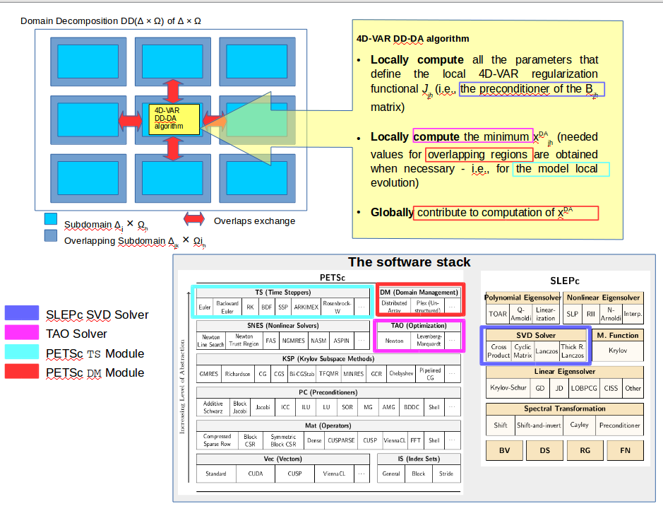
The 4D-VAR DD-DA problem solution is computed performing the following steps on each subdomains $\Delta_{j}\times\Omega_{h}$ (the so called 4D-VAR DD-DA algorithm):

• •

  Locally compute all the parameters that define the local 4D-VAR regularization functional ${J}_{jh}$

• •

  Locally compute the minimum ${\mathbf{x}}_{jh}^{DA}$ (needed values for overlapping regions are obtained when necessary - i.e., for the model local evolution)

• •

  Globally contribute to computation of ${\mathbf{x}}_{jh}^{DA}$

In order to compute the minimum of all the functionals $J_{jh}$, the DD-DA algorithm has to face with some issues. In more details, we have to address:

• •

  the linearization of the operator $\mathcal{M}_{t-\Delta t\to t}$, let us say $\mathbf{M}_{t-\Delta t}$, used for the evaluations of $J_{jh}$ required by the minimisation algorithm;

• •

  the evaluation of the adjoint operator of $\mathbf{M}_{t-\Delta t}$, let us say ${\bf M}_{t-\Delta t}^{\star}$, used for the evaluation of $\nabla J_{jh}$ required by the minimisation algorithm;

Both the points above should require the computation of the discretization of the Jacobian of $\mathcal{M}_{t-\Delta t\rightarrow t}$

Following some details about software implementation in PETSc (Portable, Extensible Toolkit for Scientific Computation)[7] environment. To implement the entire algorithm we plan to use:

1. 1.

   the PETSc time steppers TS module for solving time-dependent (nonlinear) PDEs, including the computation of adjoint;

2. 2.

   the PETSc DM module wich is a powerfull tool for the managment of all mesh data related with domain decomposition;

3. 3.

   The TAO software library [8] for the computation of (2). The Toolkit for Advanced Optimization (TAO) is aimed at the solution of large-scale optimization problems on high-performance architectures. TAO is suitable for both single-processor and massively-parallel architectures. The current version of TAO has algorithms for unconstrained and bound-constrained optimization.

4. 4.

   The SLEPc software library [9] for the computation of spectral decomposition usefull to compute a preconditioner of the error covariance matrices (i.e., see approach used in [2]). The Scalable Library for Eigenvalue Problem Computations (SLEPc) is a software library for the solution of large scale sparse eigenvalue problems on parallel computers. It can also be used for computing a partial SVD of a large, sparse, rectangular matrix, and to solve nonlinear eigenvalue problems.

All the abobe mentioned software are integrated or based on PETSc (see figure 1 for a representation of the Software stack and algorithm implementation).

To represent the Jacobian of ${\mathcal{M}}_{t-\Delta t\rightarrow t}$ in PETSc we decided to follow a “matrix-free approach”: we used a MATHSHELL type for PETSc Mat object to represent $\nabla\mathbf{M}_{t-\Delta t\rightarrow t}$ just defining its way of operating

The case study is based on the Shallow Water Equations (SWEs) on the sphere. The SWE have been used extensively as a simple model of the atmosphere or ocean circulation since they contain the essential wave propagation mechanisms found in general circulation models [1]. The SWEs in spherical coordinates are:

Here $f$ is the Coriolis parameter given by $f=2\Omega\sin{\theta}$, where $\Omega$ is the angular speed of the rotation of the Earth, $h$ is the height of the homogeneous atmosphere (or of the free ocean surface), $u$ and $v$ are the zonal and meridional wind (or the ocean velocity) components, respectively, $\theta$ and $\lambda$ are the latitudinal and longitudinal directions, respectively, $a$ is the radius of the earth and $g$ is the gravitational constant.

We express the system of equations (5)-(7) using a compact form, i.e.:

where

and

We discretize (8) just in space using an un-staggered Turkel-Zwas scheme [5, 6], and we obtain:

where

and

If we define $\mathbf{M}_{\Delta t}^{0,M_{steps}}\left(\cdot\right)$ as follows:

we note that the symbol $\mathbf{M}_{\Delta t}^{0,M_{steps}}\left(\cdot\right)$ represents the model $\mathcal{M}^{t-\Delta t\rightarrow t}_{disc}\left(\cdot\right)$ “applied” $M_{steps}$ times.

We also note that the numerical model is defined by the following parameters:

• •

  $\Delta t$ discretization step in time domain,

• •

  $\Delta\lambda$, $\Delta\theta$ discretization step in space domain,

• •

  $\alpha$ parameter of the Turkel-Zwas schema,

• •

  $p$, $q$ parameters of the Turkel-Zwas schema.

To verify the correct operation of the software module which implements the model, we tested the computed values of $\mathbf{M}_{\Delta t}^{0,M_{steps}=30}\left(x_{0}\right)$, when $\left|DD(\Delta\times\Omega)\right|=1$ (i.e., when domain $\Delta\times\Omega$ is not decomposed), where:

1. 1.

   $\Delta t=50.0,100.0,150.0,200.0$,

2. 2.

   $\alpha=\frac{1}{3}$,

3. 3.

   $p=4$ and $q=2$,

4. 4.

   $x_{0}$ is a syntetic vector containing all the considered fields: the see-level field $h$ is generated by a Gaussian stochastic process; both velocity fields $v$ and $u$ are set to zero,

5. 5.

   $\Delta\lambda$ e $\Delta\theta$ defined on the basis of discretization grid used by data available at repository Ocean Synthesis/Reanalysis Directory of Hamburg University (see [3]).

We note that the values for parameters at above mentioned points 1, 2 and 3 were chosen on the basis of the considerations and results described in [4].

In figure 2-(a) $x_{0}$ is represented. In figure 2-(b)-(d) are represented respectively $\mathbf{M}_{\Delta t}^{0,M_{steps}=30}\left(x_{0}\right)$ where $\Delta t=50.0,100.0,150.0,200.0$. We used different values for $\Delta t$ with the aim to empirically determine the “best value” for $\Delta t$. The considered values for $\Delta t$ were chosen taking into account the considerations about CFL condition for Turkel-Zwas methods described in [4].

To give a measure of how $\mathbf{M}_{\Delta t}^{0,M_{steps}=30}\left(x_{0}\right)$ differs from $x_{0}$ depending from $\Delta t$, in table 1 we show

for the considered values of $\Delta t$.

To verify the correct operation of the software module which implements the DA process we tested the computed values of $x^{\Delta t}_{DA}$, when $\left|DD(\Delta\times\Omega)\right|=1$ (i.e., when domain $\Delta\times\Omega$ is not decomposed), starting:

• •

  from the ${\bf R}_{k}={\bf R}$ ($\forall k=0,\dots,nt_{obs}-1$) diagonal matrix representing the covariance matrix of the errors on all the observations vectors

• •

  from the $H$ diagonal matrix representing the observational operator and

• •

  from the backgroud $x^{\Delta t}_{b}$ and

• •

  from the set of $nt_{obs}$ observations vectors $\left\{{}_{\Delta t}x^{n}_{obs}\right\}_{n=1,\ldots,nt_{obs}}$,

• •

  and by using, as preconditioner $\tilde{B^{\Delta t}}_{nSVs}$ of covariance matrix $B^{\Delta t}$, its Truncated SVD (the first $nSVs$ singular values $\left(S_{i}\right)_{i=0,\ldots,nSVs-1}$ of $B^{\Delta t}$ are considered),

where

1. 1.

   $x^{\Delta t}_{b}=\mathbf{M}_{\Delta t}^{0,M_{steps}=30-nt_{obs}+1}\left(x_{0}\right)$,

2. 2.

   Problem 1 For each $n=1,\ldots,nt_{obs}$, ${}_{\Delta t}x^{n}_{obs}$ $\displaystyle=$ $\displaystyle\frac{1}{10^{2}}\left[10^{2}*\mathbf{M}_{\Delta t}^{0,M_{steps}=30-nt_{obs}+n}\left(x_{0}\right)\right],$ (each elements of ${}_{\Delta t}x^{n}_{obs}$ were obtained by rounding, on the third significant digit, the respective elements of $\mathbf{M}_{\Delta t}^{0,M_{steps}=30-nt_{obs}+n}\left(x_{0}\right)$). $H$ is the identity matrix. Problem 2 For each $n=1,\ldots,nt_{obs}$, if $i$ is a multiple of $STEP=5$ $\displaystyle\left({}_{\Delta t}x^{n}_{obs}\right)_{i}$ $\displaystyle=$ $\displaystyle\left(\mathbf{M}_{\Delta t}^{0,M_{steps}=30-nt_{obs}+n}\left(x_{0}\right)\right)_{i}+0.01*randn,$ $\displaystyle diag(H)_{i}$ $\displaystyle=$ $\displaystyle 1,$ else $\displaystyle\left({}_{\Delta t}x^{n}_{obs}\right)_{i}$ $\displaystyle=$ $\displaystyle 0,$ $\displaystyle diag(H)_{i}$ $\displaystyle=$ $\displaystyle 0,$ (${}_{\Delta t}x^{n}_{obs}$ are sparse vectors whose lenght is $3*nlat*nlon$ and whose non-zero elements (the $20\%$ of the total) were obtained by adding a scaled number $0.01*randn$ from normal distribution to the respective elements of $\mathbf{M}_{\Delta t}^{0,M_{steps}=30-nt_{obs}+n}\left(x_{0}\right)$). Problem 3 For each $n=1,\ldots,nt_{obs}$, ${}_{\Delta t}x^{n}_{obs}$ $\displaystyle=$ $\displaystyle\frac{1}{10^{1}}\left[10^{1}*\mathbf{M}_{\Delta t}^{0,M_{steps}=30-nt_{obs}+n}\left(x_{0}\right)\right],$ (each elements of ${}_{\Delta t}x^{n}_{obs}$ were obtained by rounding, on the second significant digit, the respective elements of $\mathbf{M}_{\Delta t}^{0,M_{steps}=30-nt_{obs}+n}\left(x_{0}\right)$). $H$ is the identity matrix. Problem 4 For each $n=1,\ldots,nt_{obs}$, if $i$ is a multiple of $STEP=5$ $\displaystyle\left({}_{\Delta t}x^{n}_{obs}\right)_{i}$ $\displaystyle=$ $\displaystyle\left(\mathbf{M}_{\Delta t}^{0,M_{steps}=30-nt_{obs}+n}\left(x_{0}\right)\right)_{i}+0.01*O\left(\left(\mathbf{M}_{\Delta t}^{0,M_{steps}=30-nt_{obs}+n}\left(x_{0}\right)\right)_{i}\right)*randn,$ $\displaystyle diag(H)_{i}$ $\displaystyle=$ $\displaystyle 1,$ else $\displaystyle\left({}_{\Delta t}x^{n}_{obs}\right)_{i}$ $\displaystyle=$ $\displaystyle 0,$ $\displaystyle diag(H)_{i}$ $\displaystyle=$ $\displaystyle 0,$ (${}_{\Delta t}x^{n}_{obs}$ are sparse vectors whose lenght is $3*nlat*nlon$ and whose non-zero elements (the $20\%$ of the total) were obtained by adding, to the respective elements of $\mathbf{M}_{\Delta t}^{0,M_{steps}=30-nt_{obs}+n}\left(x_{0}\right)$, a number from normal distribution scaled by a factor related with order of magnitude of each elements $O\left(\left(\mathbf{M}_{\Delta t}^{0,M_{steps}=30-nt_{obs}+n}\left(x_{0}\right)\right)_{i}\right)$).

3. 3.

   $nt_{obs}=1,2,4,6,8,10$,

4. 4.

   $nSVs=4,6,8,10,12$.

5. 5.

   $\left({\bf R}^{-1}\right)_{i}=\left\{\begin{array}[]{cl}\frac{1}{1e+6}&\mbox{if\ }i=0,\ldots,nlat*nlon-1\\ 1&\mbox{if\ }i=nlat*nlon,\ldots,3*nlat*nlon\\ \end{array}\right.$.

6. 6.

   $B^{\Delta t}=\left(x^{\Delta t}_{err}\right)\left(x^{\Delta t}_{err}\right)^{T}$, where

   $$\left(x^{\Delta t}_{err}\right)_{i}=\left(x^{\Delta t}_{b}\right)_{i}-\nu^{\Delta t}$$

   and where

   $$\nu^{\Delta t}=\frac{\sum_{j=0,ldots,3*nlat*nlon-1}{\left(x^{\Delta t}_{b}\right)_{j}}}{3*nlat*nlon}$$

Figure 3 shows how the background $x^{\Delta t}_{b}$ (the red circle in the image) and observations ${}_{\Delta t}x^{n}_{obs}$ (the blue circle in the image) were chosen/built from $x^{\Delta t}_{m}=\mathbf{M}_{\Delta t}^{0,M_{steps}=m}{\left(x_{0}\right)}$ data: in particular, for each values of $nt_{obs}=1,2,4,6,8,10$, the image intends to show which subset of $\left\{x^{\Delta t}_{m}\right\}_{m=0,\ldots,30}$ is considered to generate background and observations. In particular, the procedure used to build the input data for DA problem performs the following steps:

1. 1.

   “application” of the model $\mathbf{M}_{\Delta t}^{0,M_{steps}=m}\left(\cdot\right)$ to the starting point $x_{0}$ to obtain the vector $x^{\Delta t}_{m}$ where $m=30-nt_{obs}+1$;

2. 2.

   from the vector $x^{\Delta t}_{m}$ computed at above point 1 we obtain both the background vector $x^{\Delta t}_{b}$ and, by using one of the definitions for Problem 1 or Problem 2, the first observation vector ${}_{\Delta t}x^{1}_{obs}$;

3. 3.

   further “application” of the model to compute the set of vectors $\left\{x^{\Delta t}_{m}\right\}_{m=30-nt_{obs}+2,\ldots,30}$ from which obtain, by using one of the definitions for Problem 1 or Problem 2, the remaining $nt_{obs}-1$ observation vectors ${}_{\Delta t}x^{i}_{obs},i=2,..,nt_{obs}$.

Then, the “assimilation window” $AW^{nt_{obs}}_{\Delta t}$ in time domain, when the value of ${\Delta t}$ is fixed, is the intervall defined as:

Three sets of tests are performed: the first set intends to evaluate how different values for $nt_{obs}$ and $nSVs$ influence the behavior of DA software module; the second and third sets of tests intend to give elements to evaluate how Data Assimilation used during model application (i.e., $\mathbf{M}_{\Delta t}^{0,M_{steps}=m}\left(x^{\Delta t}_{DA}\right)$) improve the quality of the model computed values without DA (i.e., $\mathbf{M}_{\Delta t}^{0,M_{steps}=m}\left(x^{\Delta t}_{b}\right)$) with respect to observations ¹¹ 1 We note that the symbols $\mathbf{M}^{0,M_{steps}=n}\left(x^{\Delta t}_{b}\right)$ and $\mathbf{M}_{\Delta t}^{0,M_{steps}=n}\left(x^{\Delta t}_{DA}\right)$ represent the model “applied” $n$ times to the background $x^{\Delta t}_{b}$ and to the solution of DA problem $x^{\Delta t}_{DA}$ respectively.

Tests Set 1 In order to evaluate how different values for $nt_{obs}$ and $nSVs$ influence the behavior of DA software module, in tables 3 (for Problem 1), 4 (for Problem 2), 5 (for Problem 3) and 6 (for Problem 4) the values of $err^{\Delta t}_{b}$ and $err^{\Delta t}_{DA}$ are showed for the above listed values of $nt_{obs}$ and $nSVs$ and for the four considered problems where

	$\displaystyle err^{\Delta t}_{b}$	$\displaystyle=$	$\displaystyle\left\|Hx^{\Delta t}_{b}-_{\Delta t}x^{n=1}_{obs}\right\|_{2}/\left\|{}_{\Delta t}x^{n=1}_{obs}\right\|_{2}$		(22)
	$\displaystyle err^{\Delta t}_{DA}$	$\displaystyle=$	$\displaystyle\left\|Hx^{\Delta t}_{DA}-_{\Delta t}x^{n=1}_{obs}\right\|_{2}/\left\|{}_{\Delta t}x^{n=1}_{obs}\right\|_{2}$		(23)

and where $\Delta t=50.0,100.0,150.0,200.0$. We note that values of $err^{\Delta t}_{DA}$ are not reported when the algorithm failed (i.e., when the Truncated SVD computation failed). The table 2 show, as examples, the values of $\left(S_{i}\right)_{i=0,\ldots,nSVs-1}$ when $nt_{obs}=2$ and $\Delta t=50.0,100.0,150.0,200.0$.

	$\left(S_{i}\right)_{i=0,\ldots,nSVs-1}$
	$\Delta t$
$i$	50.0	100.0	150.0	200.0
00	1.489436e+05	1.489436e+05	1.489436e+05	1.489436e+05
01	5.922436e-12	5.918084e-12	1.421180e-11	1.518229e-07
02	1.098639e-18	3.745277e-12	1.058226e-11	3.045052e-11
03	2.717045e-22	2.956363e-12	5.891872e-12	2.154711e-11
04	7.077415e-23	2.450420e-12	5.477584e-12	1.815192e-11
05	1.984375e-23	2.034103e-12	4.955457e-12	1.770864e-11
06	1.308422e-25	1.248364e-12	4.426257e-12	1.447040e-11
07	6.804022e-26	9.572109e-13	4.043577e-12	1.247191e-11
08	6.736329e-26	9.029654e-13	3.518900e-12	1.176448e-11
09	6.642977e-26	7.345570e-13	2.587594e-12	1.014551e-11
10	6.614099e-26	7.164269e-13	2.226629e-12	9.308843e-12
11	5.977310e-28	5.974983e-13	1.710227e-12	5.925403e-12

We also note that:

1. 1.

   the smaller values for $nSVs$ is (i.e., where $nSVs=4$), more the DA software module is able to effectively compute the solution of the DA problem;

2. 2.

   the larger values for $nSVs$ is, more accurate is the solution of the DA problem computed by DA software module (if it is successful).

This behavior could be explained considering that:

1. 1.

   the smaller the value of $nSVs$ is, better conditioned is the matrix $\tilde{B}_{nSVs}$, but also

2. 2.

   the larger values for $nSVs$ is, “closer” the matrices $\tilde{B}_{nSVs}$ and $B$ are.

		$nt_{obs}$
$\Delta t=50.0$		$1$	$2$	$4$	$6$	$8$	$10$
$err^{\Delta t}_{b}$		5.923000468033734e-03	5.918233049175874e-03	5.909744367520904e-03	5.901306860071136e-03	5.893094645517731e-03	5.884752741767643e-03
$err^{\Delta t}_{DA}$	$nSVs$
	$4$	5.923000468033728e-03	5.918233049175878e-03	5.909744367520882e-03	5.901306860071130e-03	5.893094645517735e-03	5.884752741767650e-03
	$6$	5.923000468033734e-03	5.918233049175892e-03	$-$	$-$	5.893094645517728e-03	5.884752741767642e-03
	$8$	5.923000468033734e-03	5.918233049175873e-03	5.909744367520906e-03	5.901306860071137e-03	5.893094645517726e-03	5.884752724034771e-03
	$10$	5.923000468033739e-03	5.918233049175869e-03	5.909744367520902e-03	5.901306860071123e-03	5.893094612088676e-03	5.884752741767648e-03
	$12$	$-$	5.918233049175874e-03	5.909744377775199e-03	5.901306706186256e-03	$-$	$-$

		$nt_{obs}$
$\Delta t=100.0$		$1$	$2$	$4$	$6$	$8$	$10$
$err^{\Delta t}_{b}$		6.084454299095919e-03	6.073321261976583e-03	6.052230870989613e-03	6.028625075904369e-03	6.006605050609536e-03	5.984624179759802e-03
$err^{\Delta t}_{DA}$	$nSVs$
	$4$	6.084454299095923e-03	6.073321261976588e-03	6.052230870989617e-03	6.028625075904372e-03	6.006605050609541e-03	5.984624179759798e-03
	$6$	6.084454299095920e-03	6.073321261976588e-03	6.052230870989613e-03	$-$	6.006605050609541e-03	5.984624179759808e-03
	$8$	6.084454298277842e-03	6.073321261976589e-03	6.052230870989612e-03	6.028625162320382e-03	6.006594251561000e-03	5.984624177098236e-03
	$10$	6.084454340791144e-03	$-$	6.052230870989642e-03	6.028625075904334e-03	$-$	$-$
	$12$	6.084454255839374e-03	6.073321261494072e-03	6.052230870989607e-03	6.028625075885917e-03	$-$	$-$

		$nt_{obs}$
$\Delta t=150.0$		$1$	$2$	$4$	$6$	$8$	$10$
$err^{\Delta t}_{b}$		6.280754455601023e-03	6.263201134463331e-03	6.225669222102765e-03	6.184831399882742e-03	6.143615055490961e-03	6.102356895266559e-03
$err^{\Delta t}_{DA}$	$nSVs$
	$4$	6.280754455601023e-03	6.263201134463330e-03	6.225669222102762e-03	6.184831399882739e-03	6.143615055490959e-03	6.102356895266554e-03
	$6$	6.280754455601023e-03	6.263201134463330e-03	6.225669222102764e-03	6.184831399882742e-03	$-$	6.102356895266563e-03
	$8$	6.280754455601023e-03	6.263201064275920e-03	$-$	6.184831399882738e-03	6.143615055490968e-03	6.102356895266562e-03
	$10$	6.280754446106453e-03	6.263201055314105e-03	6.225669243979252e-03	$-$	6.143615055490962e-03	6.102356790788719e-03
	$12$	6.280754387072876e-03	6.263201117930033e-03	6.225668830117284e-03	$-$	6.143615138972201e-03	6.102356811770067e-03

		$nt_{obs}$
$\Delta t=200.0$		$1$	$2$	$4$	$6$	$8$	$10$
$err^{\Delta t}_{b}$		6.462142195081026e-03	6.437375271097644e-03	6.392026891087157e-03	6.340783651666366e-03	6.292150917739605e-03	6.244798377227290e-03
$err^{\Delta t}_{DA}$	$nSVs$
	$4$	6.462142195081031e-03	6.437375271097648e-03	6.392026891087095e-03	6.340783651666372e-03	6.292150917739616e-03	6.244798377227289e-03
	$6$	6.462142195081022e-03	$-$	6.392026891087161e-03	6.340783652553978e-03	6.292150917739606e-03	6.244798377227294e-03
	$8$	$-$	6.437375271097721e-03	6.392026891087158e-03	6.340783669355231e-03	6.292150917739599e-03	6.244798377227293e-03
	$10$	$-$	6.437375294652374e-03	$-$	$-$	6.292150917739615e-03	$-$
	$12$	$-$	6.437375306111083e-03	6.392026896528792e-03	6.340783515516571e-03	$-$	$-$

		$nt_{obs}$
$\Delta t=50.0$		$1$	$2$	$4$	$6$	$8$	$10$
$err^{\Delta t}_{b}$		3.453467033333584e-02	3.496046426389585e-02	3.461814248792758e-02	3.496047407097717e-02	3.461815048663301e-02	3.496048249133105e-02
$err^{\Delta t}_{DA}$	$nSVs$
	$4$	3.453467033333583e-02	3.496046426389589e-02	3.461814248792760e-02	3.496047407097717e-02	3.461815048663298e-02	3.496048249133105e-02
	$6$	3.453467033333584e-02	3.496046426389582e-02	$-$	$-$	3.461815048663301e-02	3.496048249133105e-02
	$8$	3.453467033333584e-02	3.496046426389584e-02	3.461814248792756e-02	3.496047407097716e-02	3.461815048663301e-02	3.496048237755320e-02
	$10$	3.453467033333585e-02	3.496046426389584e-02	3.461814248792758e-02	3.496047407097717e-02	3.461815029375775e-02	3.496048249133106e-02
	$12$	$-$	3.496046426389585e-02	3.461814250679108e-02	3.496047385347141e-02	$-$	$-$

		$nt_{obs}$
$\Delta t=100.0$		$1$	$2$	$4$	$6$	$8$	$10$
$err^{\Delta t}_{b}$		3.453457238151639e-02	3.496035264638818e-02	3.461805630410621e-02	3.496039039880471e-02	3.461808760666546e-02	3.496042291664354e-02
$err^{\Delta t}_{DA}$	$nSVs$
	$4$	3.453457238151639e-02	3.496035264638819e-02	3.461805630410621e-02	3.496039039880478e-02	3.461808760666545e-02	3.496042291664356e-02
	$6$	3.453457238151640e-02	3.496035264638819e-02	3.461805630410621e-02	$-$	3.461808760666545e-02	3.496042291664352e-02
	$8$	3.453457249154981e-02	3.496035264638817e-02	3.461805630410621e-02	3.496039035077939e-02	3.461809290479863e-02	3.496042290325619e-02
	$10$	3.453457274084655e-02	$-$	3.461805630410599e-02	3.496039039880472e-02	$-$	$-$
	$12$	3.453457237819704e-02	3.496035261803864e-02	3.461805630410619e-02	3.496039039846557e-02	$-$	$-$

		$nt_{obs}$
$\Delta t=150.0$		$1$	$2$	$4$	$6$	$8$	$10$
$err^{\Delta t}_{b}$		3.453440979970871e-02	3.496017506248329e-02	3.488429733019234e-02	3.483606155320147e-02	3.461798505691022e-02	3.496032646744604e-02
$err^{\Delta t}_{DA}$	$nSVs$
	$4$	3.453440979970870e-02	3.496017506248329e-02	3.488429733019234e-02	3.483606155320147e-02	3.461798505691021e-02	3.496032646744603e-02
	$6$	3.453440979970870e-02	3.496017506248329e-02	3.488429733019234e-02	3.483606155320146e-02	$-$	3.496032646744604e-02
	$8$	3.453440979970870e-02	3.496017499975523e-02	$-$	3.483606155320146e-02	3.461798505691016e-02	3.496032646744601e-02
	$10$	3.453440976085218e-02	3.496017512611298e-02	3.488429724470573e-02	$-$	3.461798505691022e-02	3.496032641471299e-02
	$12$	3.453440988054077e-02	3.496017506439134e-02	3.488429726668655e-02	$-$	3.461798464694495e-02	3.496032654977042e-02

		$nt_{obs}$
$\Delta t=200.0$		$1$	$2$	$4$	$6$	$8$	$10$
$err^{\Delta t}_{b}$		3.453419647204346e-02	3.495994493038772e-02	3.461773231566689e-02	3.496007727466858e-02	3.496013862728978e-02	3.496019616952864e-02
$err^{\Delta t}_{DA}$	$nSVs$
	$4$	3.453419647204347e-02	3.495994493038771e-02	3.461773231566698e-02	3.496007727466857e-02	3.496013862728979e-02	3.496019616952864e-02
	$6$	3.453419647204343e-02	$-$	3.461773231566688e-02	3.496007727559594e-02	3.496013862728978e-02	3.496019616952863e-02
	$8$	$-$	3.495994493038770e-02	3.461773231566689e-02	3.496007721824784e-02	3.496013862728979e-02	3.496019616952864e-02
	$10$	$-$	3.495994489860085e-02	$-$	$-$	3.496013862728979e-02	$-$
	$12$	$-$	3.495994485406865e-02	3.461773231104990e-02	3.496007753154848e-02	$-$	$-$

		$nt_{obs}$
$\Delta t=50.0$		$1$	$2$	$4$	$6$	$8$	$10$
$err^{\Delta t}_{b}$		5.773468954018757e-02	5.773118330947371e-02	5.772450392218931e-02	5.771827398570289e-02	5.771249955261612e-02	5.770718624499813e-02
$err^{\Delta t}_{DA}$	$nSVs$
	$4$	5.773468954018757e-02	5.773118330947368e-02	5.772450392218937e-02	5.771827398570288e-02	5.771249955261611e-02	5.770718624499812e-02
	$6$	5.773468954018758e-02	5.773118330947370e-02	$-$	$-$	5.771249955261611e-02	5.770718624499811e-02
	$8$	5.773468954018757e-02	5.773118330947373e-02	5.772450392218934e-02	5.771827398570289e-02	5.771249955261611e-02	5.770718629444516e-02
	$10$	5.773468954018760e-02	5.773118330947369e-02	5.772450392218934e-02	5.771827398570289e-02	5.771249952331193e-02	5.770718624499811e-02
	$12$	$-$	5.773118330947372e-02	5.772450392378905e-02	5.771827419320513e-02	$-$	$-$

		$nt_{obs}$
$\Delta t=100.0$		$1$	$2$	$4$	$6$	$8$	$10$
$err^{\Delta t}_{b}$		5.788632535497507e-02	5.787373829705302e-02	5.784950155085092e-02	5.782658849902559e-02	5.780508422056688e-02	5.778506929509217e-02
$err^{\Delta t}_{DA}$	$nSVs$
	$4$	5.788632535497507e-02	5.787373829705301e-02	5.784950155085092e-02	5.782658849902555e-02	5.780508422056686e-02	5.778506929509220e-02
	$6$	5.788632535497510e-02	5.787373829705302e-02	5.784950155085092e-02	$-$	5.780508422056686e-02	5.778506929509220e-02
	$8$	5.788632536157578e-02	5.787373829705302e-02	5.784950155085091e-02	5.782658848730357e-02	5.780506330666032e-02	5.778506929813398e-02
	$10$	5.788632527723454e-02	$-$	5.784950155085083e-02	5.782658849902568e-02	$-$	$-$
	$12$	5.788632541333875e-02	5.787373829803212e-02	5.784950155085090e-02	5.782658849917136e-02	$-$	$-$

		$nt_{obs}$
$\Delta t=150.0$		$1$	$2$	$4$	$6$	$8$	$10$
$err^{\Delta t}_{b}$		5.809599803382869e-02	5.807549989275792e-02	5.803325570359528e-02	5.798937823866770e-02	5.794647454306275e-02	5.790575933289238e-02
$err^{\Delta t}_{DA}$	$nSVs$
	$4$	5.809599803382870e-02	5.807549989275791e-02	5.803325570359529e-02	5.798937823866770e-02	5.794647454306275e-02	5.790575933289238e-02
	$6$	5.809599803382870e-02	5.807549989275791e-02	5.803325570359529e-02	5.798937823866768e-02	$-$	5.790575933289237e-02
	$8$	5.809599803382870e-02	5.807549990183274e-02	$-$	5.798937823866769e-02	5.794647454306268e-02	5.790575933289235e-02
	$10$	5.809599807145778e-02	5.807550000874059e-02	5.803325568836281e-02	$-$	5.794647454306276e-02	5.790575939801962e-02
	$12$	5.809599805160266e-02	5.807549983114331e-02	5.803325538684955e-02	$-$	5.794647445626924e-02	5.790575931600109e-02

		$nt_{obs}$
$\Delta t=200.0$		$1$	$2$	$4$	$6$	$8$	$10$
$err^{\Delta t}_{b}$		5.830785511535787e-02	5.827839030475356e-02	5.822099874390471e-02	5.816499040667799e-02	5.810964168493156e-02	5.805455701855686e-02
$err^{\Delta t}_{DA}$	$nSVs$
	$4$	5.830785511535792e-02	5.827839030475357e-02	5.822099874390501e-02	5.816499040667800e-02	5.810964168493161e-02	5.805455701855686e-02
	$6$	5.830785511535794e-02	$-$	5.822099874390471e-02	5.816499040727242e-02	5.810964168493156e-02	5.805455701855683e-02
	$8$	$-$	5.827839030475357e-02	5.822099874390473e-02	5.816499039611871e-02	5.810964168493157e-02	5.805455701855686e-02
	$10$	$-$	5.827839030296449e-02	$-$	$-$	5.810964168493159e-02	$-$
	$12$	$-$	5.827839029079828e-02	5.822099874092245e-02	5.816499015380254e-02	$-$	$-$

		$nt_{obs}$
$\Delta t=50.0$		$1$	$2$	$4$	$6$	$8$	$10$
$err^{\Delta t}_{b}$		3.212944523284356e-02	3.146374761827107e-02	2.712145713499754e-02	3.057501318054897e-02	2.712146361761048e-02	3.057501994577008e-02
$err^{\Delta t}_{DA}$	$nSVs$
	$4$	3.212944523284356e-02	3.146374761827107e-02	2.712145713499750e-02	3.057501318054896e-02	2.712146361761048e-02	3.057501994577008e-02
	$6$	3.212944523284356e-02	3.146374761827107e-02	$-$	$-$	2.712146361761048e-02	3.057501994577008e-02
	$8$	3.212944523284356e-02	3.146374761827107e-02	2.712145713499755e-02	3.057501318054896e-02	2.712146361761049e-02	3.057502001608988e-02
	$10$	3.212944523284356e-02	3.146374761827108e-02	2.712145713499754e-02	3.057501318054895e-02	2.712146366967664e-02	3.057501994577007e-02
	$12$	$-$	3.146374761827107e-02	2.712145708523746e-02	3.057501359781360e-02	$-$	$-$

		$nt_{obs}$
$\Delta t=100.0$		$1$	$2$	$4$	$6$	$8$	$10$
$err^{\Delta t}_{b}$		3.212934767372494e-02	3.146365882582471e-02	2.712139102136180e-02	3.057494708253965e-02	2.712141382551856e-02	3.057497214505261e-02
$err^{\Delta t}_{DA}$	$nSVs$
	$4$	3.212934767372495e-02	3.146365882582471e-02	2.712139102136180e-02	3.057494708253973e-02	2.712141382551856e-02	3.057497214505259e-02
	$6$	3.212934767372496e-02	3.146365882582471e-02	2.712139102136180e-02	$-$	2.712141382551856e-02	3.057497214505262e-02
	$8$	3.212934776080620e-02	3.146365882582471e-02	2.712139102136179e-02	3.057494706301675e-02	2.712144164470810e-02	3.057497214657582e-02
	$10$	3.212934748665278e-02	$-$	2.712139102136160e-02	3.057494708253960e-02	$-$	$-$
	$12$	3.212934758819253e-02	3.146365881283841e-02	2.712139102136179e-02	3.057494708234279e-02	$-$	$-$

		$nt_{obs}$
$\Delta t=150.0$		$1$	$2$	$4$	$6$	$8$	$10$
$err^{\Delta t}_{b}$		2.983871447550081e-02	2.728177997180958e-02	2.906807057721612e-02	3.146357791255923e-02	2.712133412057428e-02	3.057489714184252e-02
$err^{\Delta t}_{DA}$	$nSVs$
	$4$	2.983871447550081e-02	2.728177997180958e-02	2.906807057721612e-02	3.146357791255922e-02	2.712133412057427e-02	3.057489714184253e-02
	$6$	2.983871447550081e-02	2.728177997180958e-02	2.906807057721612e-02	3.146357791255922e-02	$-$	3.057489714184252e-02
	$8$	2.983871447550081e-02	2.728177987323344e-02	$-$	3.146357791255923e-02	2.712133412057424e-02	3.057489714184251e-02
	$10$	2.983871441410072e-02	2.728178024259760e-02	2.906807054678072e-02	$-$	2.712133412057428e-02	3.057489704777779e-02
	$12$	2.983871463090574e-02	2.728178016178572e-02	2.906806976987517e-02	$-$	2.712133508936694e-02	3.057489710667452e-02

		$nt_{obs}$
$\Delta t=200.0$		$1$	$2$	$4$	$6$	$8$	$10$
$err^{\Delta t}_{b}$		3.212898155458577e-02	3.146332038022308e-02	2.712113568922558e-02	3.057469532393129e-02	3.057474522264301e-02	3.057479199381502e-02
$err^{\Delta t}_{DA}$	$nSVs$
	$4$	3.212898155458578e-02	3.146332038022308e-02	2.712113568922544e-02	3.057469532393129e-02	3.057474522264302e-02	3.057479199381503e-02
	$6$	3.212898155458573e-02	$-$	2.712113568922558e-02	3.057469532852141e-02	3.057474522264301e-02	3.057479199381503e-02
	$8$	$-$	3.146332038022306e-02	2.712113568922558e-02	3.057469537977613e-02	3.057474522264301e-02	3.057479199381503e-02
	$10$	$-$	3.146332040002525e-02	$-$	$-$	3.057474522264301e-02	$-$
	$12$	$-$	3.146332042802096e-02	2.712113568750191e-02	3.057469542330091e-02	$-$	$-$

Tests Set 2 In order to evaluate how the use of the Data Assimilation influences the model’s performance, in figures 4, 5, 6 and 7 trends of

$$\|H\mathbf{M}_{\Delta t}^{0,M_{steps}=n}\left(x^{\Delta t}_{DA}\right)-_{\Delta t}x^{n+1}_{obs}\|_{2}/\left\|{}_{\Delta t}x^{n+1}_{obs}\right\|_{2}$$

and

$$\|H\mathbf{M}^{0,M_{steps}=n}\left(x^{\Delta t}_{b}\right)-_{\Delta t}x^{n+1}_{obs}\|_{2}/\left\|{}_{\Delta t}x^{n+1}_{obs}\right\|_{2}$$

as functions of $n=0,\ldots,nt_{obs}-1$ are showed (values of $nt_{obs}$ and $nSVs$ are fixed and their values are $nt_{obs}=10$ e $nSVs=4$, (a)-(d)-labeled plots are related with Problems 1-4 respectively). It seems that the use of DA positively influences the model performance just for Problems 1 and 3: such influence is more significant if greater is the value of $\Delta t$.

(a)	(c)
(b)	(d)

(a)	(c)
(b)	(d)

(a)	(c)
(b)	(d)

(a)	(c)
(b)	(d)

Tests Set 3 In order to evaluate how the use of 4DVAR approach (which use a number of observations vectors $nt_{obs}$ greater than $1$) influences the model’s performance, in figures 8, 9, 10 and 11, trends of

$$\|H\mathbf{M}_{\Delta t}^{0,M_{steps}=n}\left(x^{\Delta t}_{DA}\right)-_{\Delta t}x^{n+1}_{obs}\|_{2}/\left\|{}_{\Delta t}x^{n+1}_{obs}\right\|_{2}$$

and

$$\|H\mathbf{M}^{0,M_{steps}=n}\left(x^{\Delta t}_{b}\right)-_{\Delta t}x^{n+1}_{obs}\|_{2}/\left\|{}_{\Delta t}x^{n+1}_{obs}\right\|_{2}$$

as functions of $n=0,\ldots,nt_{obs}-1$ are compared when $nt_{obs}=2,6,10$ (the value of $nSVs$ is fixed and its value is $nSVs=4$, (a)-(d)-labeled plots are related with Problems 1-4 respectively). It seems that the use of a number of observations $nt_{obs}$ greater than $1$ doesn’t significantly influence the model performance so it may not be convenient to use multiple observations (indeed, the computational cost of the DA algorithm increases with $nt_{obs}$).

References

• [1] A. St-Cyr, C. Jablonowski, J. M. Dennis, H. M. Tufo, and S. J. Thomas, A comparison of two shallow water models with nonconforming adaptive grids. Monthly Weather Review, Vol. 136, pp. 1898-1922, 2008.
• [2] D’Amore, L., Arcucci, R., Carracciuolo, L., Murli, A., A Scalable approach for variational data assimilation, (2014) Journal of Scientific Computing, 61 (2), pp. 239-257. DOI: 10.1007/s10915-014-9824-2
• [3] ECMWF Ocean ReAnalysis ORA-S3,
Avalaible at: http://icdc.cen.uni-hamburg.de/projekte/easy-init/easy-init-ocean.html
• [4] B Neta, F.X Giraldo, I.M Navon, Analysis of the Turkel-Zwas Scheme for the Two-Dimensional Shallow Water Equations in Spherical Coordinates, Journal of Computational Physics, Volume 133, Issue 1, 1997, Pages 102-112, ISSN 0021-9991, http://dx.doi.org/10.1006/jcph.1997.5657.
• [5] I. M. Navon and R. De Villiers, The application of the Turkel-Zwas explicit large time-step scheme to a hemispheric barotropic model with constraint restoration, Monthly Weather Review, Vol. 115(5), pp. 1036-1052, 1987.
• [6] I. M. Navon and J. Yu, Exshall: A Turkel-Zwas explicit large time-step FORTRAN program for solving the shallow-water equations in spherical coordinates, Computers and Geosciences, Vol. 17(9), pp. 1311-1343, 1991.
• [7] S. Balay, S. Abhyankar, M.F. Adams, J. Brown, P. Brune, K. Buschelman, V. Eijkhout, W.D. Gropp, D. Kaushik, M.G. Knepley, L. Curfman McInnes, K. Rupp, B.F. Smith and H. Zhang, PETSc Users Manual, ANL-95/11 Revision 3.7, Argonne National Laboratory,
• [8] Todd Munson, Jason Sarich, Stefan Wild, Steven Benson, Lois Curfman McInnes, TAO 2.0 Users Manual, ANL/MCS-TM-322, Mathematics and Computer Science Division of the Argonne National Laboratory, 2012.
• [9] V. Hernandez, J. E. Roman, and V. Vidal. SLEPc: A scalable and flexible toolkit for the solution of eigenvalue problems, ACM Trans. Math. Software, 31(3):351-362, 2005.