Efficient Detectors for MIMO-OFDM Systems under Spatial Correlation Antenna Arrays
Abstract
This work analyzes the performance of the implementable detectors for multiple-input-multiple-output (MIMO) orthogonal frequency division multiplexing (OFDM) technique under specific and realistic operation system conditions, including antenna correlation and array configuration. Time-domain channel model has been used to evaluate the system performance under realistic communication channel and system scenarios, including different channel correlation, modulation order and antenna arrays configurations. A bunch of MIMO-OFDM detectors were analyzed for the purpose of achieve high performance combined with high capacity systems and manageable computational complexity. Numerical Monte-Carlo simulations (MCS) demonstrate the channel selectivity effect, while the impact of the number of antennas, adoption of linear against heuristic-based detection schemes, and the spatial correlation effect under linear and planar antenna arrays are analyzed in the MIMO-OFDM context.
Index Terms:
MIMO-OFDM; multipath channel; Jakes modified model; linear detector; heuristic detector; spatial correlation; BER performance.I Introduction
OFDM is a modulation scheme widely used in many communication systems, including several commercial applications such as wireless networks (Wi-Fi 802.11) and cellular systems (LTE) [1]. In those systems, it is also common to combine the OFDM with Multiple Input Multiple Output (MIMO), which can improve the spectral efficiency of the system [2], [3]. However, to couple the OFDM to the MIMO system, it is necessary to understand the basics of SISO channel and SISO OFDM.
Usually, inside an OFDM system, a large number of subcarriers is deployed in order to achieve a flat fading condition on each subchannel. This is particularly important in realistic scenarios, where wireless channel introduces dispersion effects on the signal, creating selective channels. In [4], a SISO OFDM system was simulated to show how the number of subcarriers influence its performance on a multipath fading indoor channel based on Saleh-Valenzuela model, but not considering the Doppler frequency.
In flat fading channels, the coherence bandwidth of the channel is larger than the bandwidth of the signal, . Hence, all frequency components of the signal will experience the same magnitude of fading. On the other hand, in frequency-selective fading channels occurs. As a consequence, different frequency components of the signal experience correlated fading.
In order to verify the influence of the number of subcarriers on the system performance, the system must operate in multipath channels. In the literature, some channel models are described in time domain (TD), e.g. Jakes model [5], while other in frequency domain (FD), such as Clarke-Gans model [6]. In this article, the Jakes modified model proposed in [7] is deployed. This TD channel simulator model performs a sum of cosines with random phases, multiplied by Walsh-Hadamard coefficients such that each waveform becomes uncorrelated. In this model, the frequency Doppler is considered, i.e., the mobility of the user terminal (UT) is taken into account aiming to analyze more realistic mobile radio scenarios.
In OFDM systems, to mitigate the inter-symbol interference (ISI) caused by multipath fading, it is necessary the use of guard interval. The most used type of guard interval on OFDM systems is the cyclic prefix (CP), as described analytically in [8].
One of the most recent well-established data transmission structure is multiple-input multiple-output (MIMO) system, which use multiple antennas at the transmitter and receiver sides to transfer data over a wire or wireless channels. MIMO systems are able to increase data rates by means of multiplexing or to improve performance/reliability through diversity mode [9]. The data increase can be achieved sending different data via different antennas. Sending simultaneously the same data via multiple antennas the reliability are increased exploiting diversities, such as time and space diversity. In spatial multiplexing, the signal that reaches at each receive antenna is interfered by the others antennas, where represents the number of transmitting antennas. So, the purpose of demultiplexing-detection schemes is to mitigate the effects of the interference [10]. Hence, on the receive side, there is a large number of MIMO detection techniques available. In this work, a bunch of MIMO-OFDM detectors are characterized and numerically evaluated under specific but realistic channel and system scenarios, including: the maximum likelihood (ML), the linear zero forcing (ZF) and the linear minimum mean square error (MMSE) detectors. Moreover, two MIMO-OFDM detectors based on the evolutionary heuristic approaches also have been analyzed, namely the particle swarm optimization (PSO) detector, and differential evolution (DE) detector.
Indeed, since the ML detector solution requires an exhaustive search going through all possible symbols combinations [11], while linear closed solutions such as ZF and MMSE result in a poor performance for highly correlated channels [12], evolutionary heuristic algorithms are strong candidates to produce better solutions compared with linear detectors, and they results in reduced computational complexity compared to ML, since heuristic approaches do not evaluate all possibilities.
The PSO algorithm was already applied to solve the detection problem in MIMO-OFDM systems in [11, 13]. In [11], the PSO and in [14] the binary PSO (BPSO) are evaluated and numerical results of BER and computational complexity are analyzed. In [13], the performances of DE, PSO and genetic algorithm (GA) are compared. On the other hand, in our work, the performance-complexity tradeoff of the evolutionary heuristic PSO and DE MIMO-OFDM detectors are analyzed under practical and useful scenarios, i.e., considering spatial correlated channels and other linear conventional MIMO-OFDM detectors. The system model in the real-valued representation is considered while the selection procedure for the heuristic input parameters of PSO and DE algorithms are addressed accordingly. Besides, to the best of our knowledge, there are no works considering a comparative analysis of evolutionary heuristics and classical MIMO-OFDM detectors operating under spatial correlation antenna arrays.
The contribution of this work is threefold. a) Firstly, we analyze and compare a bunch of MIMO-OFDM detectors, including linear and evolutionary heuristic approaches, operating under realistic system configurations, regarding performance and implementability. b) Second, the influence of parameters related to the distance between the antennas, which determine the spatial antenna correlation, is discussed; two antenna arrays configurations are considered, the uniform linear array (ULA) [15] and the uniform rectangular array (URA) [16]. c) Last, a systematic procedure is developed and used to calibrate the input parameters of both evolutionary heuristic PSO and DE detectors aiming at establishing a fair performance comparison between the linear and heuristic MIMO-OFDM detectors.
The rest of this work is organized as follows. In section II, the OFDM system is revised, and time-domain channel emulator is explored, including details of modified Jakes channel model. Descriptions for the spatial channel correlation, the ML, ZF, MMSE, as well as the evolutionary heuristic PSO and DE detectors are developed in section III. Extensive numerical simulation results are analyzed in section V, including reliability evaluation, channel selectivity effect, bit error rate (BER) performance comparison regarding spatial correlation, modulation order and sensibility analysis as well. Conclusions and final remarks are offered in VI.
Notation: and represent, respectively, the Fourier transform and the inverse Fourier transform; represents convolution operator. represents Hermitian operator. means Frobenius norm, expectation operator; bold lowercase letter represents a vector, while bold capital letter represents matrix. and operators represent the real and imaginary parts of a complex number. Operator denotes Hadamard product, while is the Kronecker product.
II OFDM Transmission and MIMO Channel
OFDM is one type of multicarrier modulation that can be easily implemented using discrete Fourier transform (DFT) and its inverse (IDFT), or their equivalents fast Fourier transform (FFT) and inverse fast Fourier transform (IFFT). OFDM modulation consists in parallel data transmission with some modulation as M-QAM, M-PSK, etc, applying an IFFT to pass the signal of frequency domain to time domain. Thereafter, the cyclic prefix is added. Data is converted to an analogical signal. And finally, the signal is multiplied to a carrier with frequency to transmit.
On the receiver side, the signal represents the transmitted signal corrupted by noise. The signal is multiplied by , pass through a low-pass filter (LPF), then, the signal is converted to digital information, the cyclic prefix is removed and the serial data is converted to parallel. The DFT is performed, the symbols are converted to serial and demodulated to its respective scheme of modulation and the information bits can be estimated.
In order to mitigate intersymbol interference (ISI), some strategies, such as cyclic suffix, silence or the most common cyclic prefix (CP) can be adopted. CP consists in copying the last elements of the input sequence and adding them to the start of , where represents the channel impulse response, with length . After the CP addition, OFDM symbol becomes , with length . Observe that the CP is an overhead, not carrying any information, which reduces the spectral efficiency.
The choice of the number of subcarriers () depends on the channel characteristics. For the design of an OFDM system, it is considered two properties of the channel, which are the maximum delay spread () and maximum Doppler frequency . OFDM systems require that must be large enough so each subcarrier experiences a flat fading condition. Each subcarrier has a bandwidth smaller than the system total bandwidth, centered at a frequency . Subcarriers bandwidth of can be overlapped at a maximum rate of 50%.
II-A MIMO-OFDM System
The combination of the OFDM system with the use multiple antennas at the transmitter and receiver results in MIMO-OFDM system, Fig. 1, with transmit and received antennas. QAM modulator and multiplexing configuration, i.e., different data is sent through different antennas resulting in higher data rates than single-input-single-output (SISO) channel configuration have been considered.
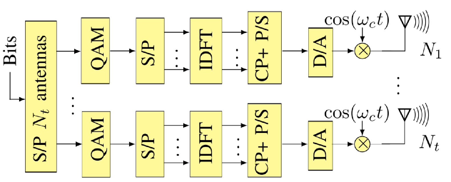
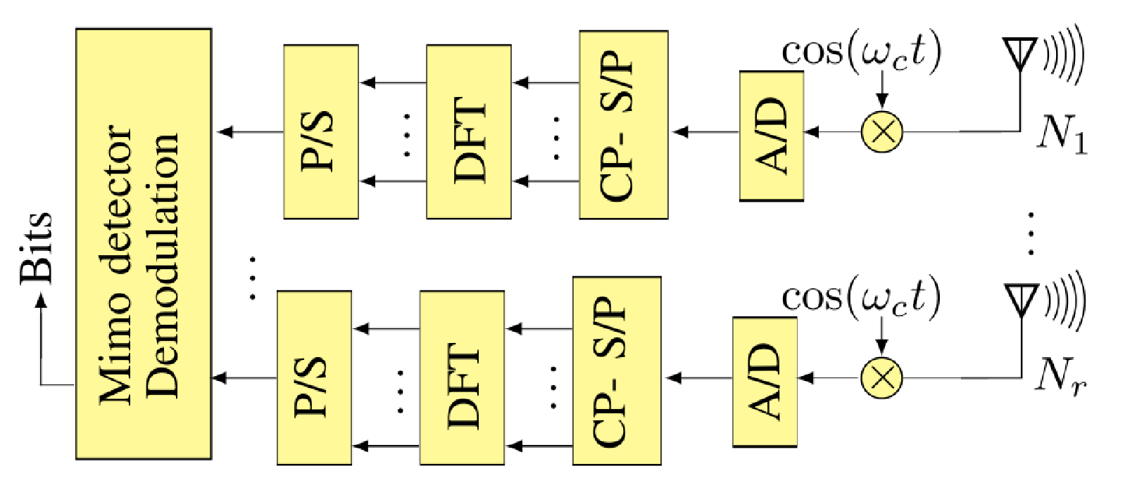
On the transmitter side, the data feeds a serial-to-parallel converter, resulting in data streams, that are modulated in a similar way as OFDM SISO: the bit stream is modulated, the symbols are converted to parallel, the IDFT is performed, the cyclic prefix is added, the signal is multiplied by the carrier with frequency and finally transmitted. On the receiver side, the signal is converted to baseband, transformed to digital, the cyclic prefix is removed, and the signals serve a MIMO detector, and finally, the symbols are demodulated deploying QAM demodulator.
As the OFDM technique allows parallel transmission over several subchannels, we can model a MIMO-OFDM system with subcarriers in time domain as [17], [18]:
| (1) |
where is the subcarrier index; is the received signals, is the channel matrix gains; is the transmit symbols and is the Gaussian noise with zero mean and variance .
Therefore, we can interpret a MIMO system for each subcarrier, as illustrated in Fig. 2. Thus, a MIMO-OFDM symbol block is composed of OFDM symbols. Finally, it is important to note that if the number of subcarriers is insufficient to make the channel of each subcarrier flat, channel equalization can not be implemented correctly.

Implementable MIMO-OFDM detectors operating in realistic fading channels and practical system configuration are discussed in Section III.
II-B Wireless Channel
The noise is represented in time domain as it taken in account after the IDFT operation. In TD, fading interference can be written as a convolution operation of the channel impulse response with the transmitter’s signal , which can be represented with discrete sequences:
| (2) |
The original information can be recovered analyzing the operation in FD, using the Fourier transform convolution property:
| (3) |
Two important parameters in a wireless channel are the coherence time and the coherence band . They are related to maximum Doppler frequency () and root-mean-square delay spread (), respectively.
| (4) |
The number of subcarriers in an OFDM system is defined by the channel’s characteristics given in terms of delay spread, which can be observed experimentally via power delay profile (PDP), a graph that represents the channel parameters of power versus delay.
The PDP used in this work is the IEEE 802.11b, characterized by a decreasing exponential behaviour. The implementation of this channel model is discussed in several works in the literature, e.g., [19].
II-C Modified Jakes Channel Model
In [20], Jakes discusses statistical properties of wireless channels. The mathematical model described in time domain, namely Jakes model, performs a sum of cosines with angles uniformly distributed and considers mobility of Tx-Rx via the maximum Doppler shift effect. Twenty years later, Dent et al [7] proposed improvements on the Jakes model, known as Jakes modified (JM) model. In this model, a factor subtraction of is suggested to eliminate the singular angles and [rad], while the multiplication of the fading samples by Walsh-Hadamard coefficients is indicated to generate uncorrelated channel waveforms. Herein, both the amplitude and phase of fading samples are analyzed and the JM model is implemented and applied to the analysis of OFDM systems.
To generate uncorrelated channel waveforms with Jakes modified model, the following relation must be respected:
| (5) |
where represents the -th Walsh-Hadamard (WH) coefficient, generated via WH matrices [21], is the number of oscillators, and ,
| (6) | |||
| (7) | |||
| (8) | |||
| (9) |
The autocorrelation function of the fading channel samples generated via JM method follows the Bessel function of first kind and 0th order:
| (10) |
By applying the Fourier transform on the autocorrelation function, power spectrum density (PSD) can be derived:
| (11) |
III MIMO Spatial Correlation and Linear Detectors
III-A MIMO-OFDM Spatial Correlation Model
In channel modelling, the correlation among transmit and/or receive antennas is an important aspect to be considered in realistic MIMO channels and systems [19]. To model and evaluate the spatial antenna correlation, the Kronecker operator is deployed as:
| (12) |
where is the correlated channel of the nth subcarrier, uncorrelated channel matrix is composed by independent and identically distributed (i.i.d.) entries, and are the square root of the spatial correlation matrices at the transmitter and receiver antennas, respectively.
III-B Uniform Linear Antenna Array (ULA)
A spatial correlation model for ULA is proposed in [15]. This model considers that the antennas are arranged equidistantly, where and represent the spacing between the transmitting and receiving antennas, respectively. For simplicity of analysis, assuming the same number of antennas at the transmitter and receiver () side, while the spatial correlation matrix of the transmitter and receiver antennas are assumed equals (). The spatial correlation matrix results Toeplitz, being expressed by:
| (13) |
where represents the normalised correlation index between the antennas.
III-C Uniform Rectangular Antenna Array (URA)
An aproximation for the URA correlation model is proposed in [16]. This model gives that the URA matrix correlation between the antennas is obtained from the Kronecker product of two ULA correlation matrices. Considering an URA configuration on the XY plane, with and antenna elements along X and Y coordinates, respectively, so we have an array with antennas. Considering that the correlation between the elements along X coordinate does not depend on Y and is given by matrix , and the correlation along Y coordinate does not depend on X and is given by matrix . As a result, the Kronecker model approximation for the URA correlation matrix follows:
| (14) |
III-D Maximum likelihood (ML) MIMO Detector
The ML detector provides the best performance between the detectors, but its complexity makes it impractical for real applications. This detector calculates all the possible symbols combinations and choose the one symbol vector which provides the minimum Euclidian distance between the received data and the reconstructed one defined by the channel matrix and the symbol-vector candidate . Hence, the estimated symbol can be mathematically expressed by:
| (15) |
III-E Zero-Forcing (ZF) MIMO Detector
Considering a MIMO system operating under multiplexing mode, the data that reaches the receptor is the linear superposition of the signals of all the antennas [10]. The ZF detector ignores the additive noise z in eq. (1) and solves the linear system multiplying the received signal by the inverse matrix which is defined, according to Moore-Penrose inverse matrix, as:
| (16) |
The estimated symbol is given by:
| (17) |
III-F Minimum Mean Square Error (MMSE) MIMO Detector
The MMSE detector considers the thermal noise channel statistics. This method tries to minimize the squared error between the true and estimated values of the transmitted symbols, and , respectively [10] via optimisation
| (18) |
Hence, solving this MMSE optimisation problem, the MIMO channel matrix results in the MMSE pseudo-inverse matrix described as:
| (19) |
where is the inverse of the signal-to-noise ratio (SNR). Finally, the estimated symbol under linear MMSE MIMO detection is obtained in the same way of (16), and given by:
| (20) |
IV Heuristic-based MIMO-OFDM Detectors
In this section, the heuristic PSO and DE algorithms are described in the context of the MIMO-OFDM detection problem. The complex system model is described in a well-known equivalent real-valued representation, e.g. [22]. The deployment of the fitness function to evaluate the candidate-solution provided by heuristic algorithms is illustrated. PSO and DE algorithms are presented in the sequel, while the input parameters tuning problem for the evolutionary heuristic algorithms is addressed.
IV-1 Real Value Representation
The MIMO-OFDM system presented in eq. (1) can be represented as real-valued matrix and vectors in the form:
| (21) |
with:
where is the real-valued representation of the channel matrix, vectors are the real-valued representations of the original information and additive noise, respectively, and the real-valued received signal.
IV-2 Fitness Function
The fitness function evaluates the quality of the estimated symbol and guides the evolutionary heuristic search on the candidate-solution feaseable subspace. For detection problem, the fitness function is based on the Euclidean distance between the received signal and the reconstructed one [13, 11, 14]. Considering the th candidate-solution of a evolutionary heuristic, , namely particle in PSO or individual in DE, the fitness function is calculated as:
| (22) |
For the detection problem, a minimization problem is considered and lower values of fitness function are desired.
IV-A PSO-based Detection Algorithm
PSO was proposed by [23] considering a population-based approach, emulating bird flocking and fish schooling behavior. The PSO algorithm performs calculation of velocity and position of each particle inside the swarm; using matrix representation [24], they are given respectively by:
| (23) |
| (24) |
where represent inertia, cognitive and social factors, respectively; and are random matrices with elements following uniform distributions ; is a matrix that store values of personal best of each particle and is a matrix constructed with the positions of the global best particle , given in the form . is a real-valued matrix representing positions, while represents particle velocity matrix; explicitly:
where vectors with represent the position and velocity of the kth particle, with representing the population size and the dimensionality of the problem.
In order to avoid a possibly grow to infinity of the velocity vector [25], the limitation of velocity [26] was considered, where represents the maximum achievable velocity of the particles. Regard the inertia parameter, it can be a constant, a linear or nonlinear function [27]. In this work, in order to give to the algorithm exploitation ability at the beginning and exploration to fine search the solution [26], a decreasing strategy at each iteration of the inertia factor given by is considered.
The initialization of the both implemented PSO and DE heuristic algorithms was the same; the position of the particles and initial population in DE are generated randomly following an uniform distribution inside the search space of the problem [28]. Those positions are set as the personal best position of the particle in the matrix . The fitness function in eq. (22) is evaluated () and the position of the particle that produces the lowest value (since we are dealing with a minimization problem) is set as the global best position , and the matrix is formed.
After evaluation of eq. (23) and eq.(24), matrices and are updated (if needed) and the process is repeated till the stop criteria is met. In our implementation, the stop criterion based on the pre-defined maximum number of evaluations is considered. Hence, after iterations, the output of the evolutionary heuristic algorithm is the vector of the best position , which is the estimated symbol in the MIMO-OFDM detection problem.
A pseudocode summarizing the procedure for the evolutionary heuristic PSO algorithm is presented in Algorithm 1.
IV-B DE-based Detection Algorithm
The differential evolution (DE) is an evolutionary population-based heuristic that relies on a population of individuals to find global optima. The algorithm relies on operations of mutation, crossover and selection to produce more suitable individuals through generations.
The DE algorithm was presented in [28] and operates as follows. There are vectors of individuals that are represented as , where represents the dimensionality of the problem. Herein, following the procedure defined in [28], the rand/1/bin strategy is employed. Strategies to scape to local optima adopted in DE-based detector are described in the following.
- a)
Mutation: The -th mutation vector is constructed as:
(25) where , . Variables are integer random indexes uniformly distributed inside the interval and represents the mutation scale factor.
- b)
Crossover: The -th crossover vector () is constructed as following. The -th element, , of the -th crossover vector is selected given the following rule:
(26) where ; is an integer randomly generated in the interval ; the crossover factor is defined by . As pointed out in [28], the crossover vector has at least one element from the mutation vector, i.e., the condition .
- c)
Selection: The next generation of individuals is constructed as:
(27) The fitness function in eq.(22) evaluates and . Vectors that produce more suitable values (smaller values) are selected and a new generation of individuals is produced.
After the execution of iterations, the best individual, in other words, the individual corresponding to the lowest value of fitness function in eq. (22) is the output of the algorithm, and the estimated symbol of the MIMO-OFDM detection problem. A pseudocode synthesizing DE steps is presented in Algorithm 2.
IV-C Input Parameters
The non-optimal input parameter values choice could substantially degrade the performance results provided by the heuristic algorithm in a given application, as studied in [29] for Ant-Colony Optimization algorithm. Besides, PSO algorithm also suffers alteration of convergence properties when input parameters are chosen incorrectly [25, 30, 31]. In a same way, the DE-based algorithm has some recommended interval of values to achieve fast convergence with DE algorithm [28]. For instance, the number of individuals must be in between , where is the problem dimension, as suggested in [28].
In order to provide a fair comparison between the selected evolutionary heuristic algorithms, and since the such approach are sensible to the choice of the input parameter values, which can differ substantially considering different optimization problems nature, the input parameter tuning procedure herein is obtained numerically, and discussed in subsections V-D1 and V-D2.
V Numerical Results
The OFDM scheme is numerically simulated at equivalent baseband frequencies and the associated performance evaluated and analyzed with respect to the number of subcarriers, modulation order and different SNR regions. For the simulation of OFDM system, a system with -QAM, -QAM and -QAM modulation formats has been considered. The number of subcarriers was increased and the system performance in terms of BER versus analyzed. After the verification in terms of subcarriers number and prefix cyclic, numerical simulation results of MIMO-OFDM system are discussed. In this case, specifically linear and evolutionary heuristic detectors performance subject to spatial antenna correlation effect has been compared.
V-A Statistical Characteristics for Jakes Model Fading
In this subsection samples generated by the implemented JM method is analyzed in order to verify whether or not their statistical properties are compatible with the theoretical channel model.
| Parameter | Value |
|---|---|
| # oscillators | |
| noise samples | 16384 |
| Doppler frequency | Hz |
| sampling period | s |
| waveforms | 4 |
The JM fading characteristics are presented in Fig. 3, which were generated using the JM parameters listed in Table I. In these plots, the behaviour of only one channel path waveform is depicted, since the statistical properties was similar for the other waveforms. As it can be observed, the module’s probability density function followed a Rayleigh distribution, while the phase variable follows an uniform distribution with values between to . Also, The obtained autocorrelation function corroborates the theoretical Bessel 0-th order function; as expected, the PSD peaks were located at frequencies and , with Hz, for convenience.

V-B OFDM Performance under (non)-Selective JM Channel Generator
After observing that the generated samples are statistically consistent with the Jakes modified model and PDP described in [19], the BER performance varying the number of subcarriers was analyzed. It was simulated an OFDM system with 16-QAM and fading channel samples obtained from the JM model, where the number of subcarriers was varied from a selective sub-channel basis condition to a totally flat channel condition over each OFDM sub-channel. Curves for the BER performance are depicted in Fig. 4. The associated system parameters deployed in the simulation are summarized in Table II. Indeed, we have considered a realistic scenario with OFDM system bandwidth MHz, delay spread s and a low-median mobility, resulting in a maximum Doppler frequency of Hz. Hence, the coherence time and the coherence bandwidth are readily determined by eq. (4).
| Parameter | Value |
|---|---|
| # oscillators | |
| Max. Doppler frequency | Hz |
| Jakes mod. sampling period | |
| System Bandwidth | MHz |
| # Subcarriers (N) | 64, 128, 256, 512, 1024 |
| 2.5 s | |
| PDP | IEEE 802.11b |
Since the fading coefficients are generated in time domain, the circular convolution operation was performed between the coefficients in time domain (after IFFT operation) and JM fading coefficients. The fading effect was removed using eq. (3).
As it can be observed in Fig. 4 the BER performance of the system under such circumstances increases as the number of subcarriers grows. Also, the number of subcarriers for flatness condition of course depends on the coherence bandwidth of the channel. If the number is large enough, , the flat channel condition is achieved.
Deploying quadrature amplitude modulation of -ary order (-QAM), the BER performance of a OFDM system operating under fading channel tends to the -QAM BER at Rayleigh fading channel. Analytical expression for -QAM performance under fading channel is presented in [19].

Relating the coherence bandwidth with number of subcarriers, the flatness condition in OFDM subchannel is achieved if:
For practical purpose, one can assume that the bandwidth of the OFDM subchannel is five times less than the coherence bandwidth:
From eq. (4) one can define the minimum number of subcarrier for flatness condition:

V-C OFDM Performance under (non)-Selective JM Channel Model with different CP Sizes
Considering the same scenario of the previous subsection with system bandwidth MHz, delay spread s, the impact of cyclic prefix (CP) sizes on the OFDM performance is depicted in Fig. 6.
As shown in Fig. 4, the system achieve the flatness channel condition with subcarriers. When an excessive CP size is used (around 20%), the performance of the system with 256 subcarriers approaches the performance of single-carrier flat fading condition. However, since the number of subcarrier is not enough for the OFDM system achieve the flatness condition, the system will present a limited performance, because selectivity of the channel in each subcarrier. Moreover the reduction in the CP size causes the OFDM inter-symbol interference (ISI), degrading the performance, i.e., even for an increase of SNR the BER performance remained virtually the same (BER floor effect).

Indeed, in flat channel condition ( subcarriers), note that the system performance tends to deteriorate with decreasing of CP size. The system has about the same performance for all the considered values of CP, however, when the CP size is insufficient to combat ISI, which occurs for a CP around 10% of OFDM period, the system starts to show a BER floor (limitation), whereas an increase in no longer provides a significant performance increase (decreased BER). However, if the CP size is very large we will be expending energy unnecessarily, because the CP increases the OFDM period to combat ISI and therefore waste energy to do this. From Fig. 6,one should use a CP size from 12.5 % to 15 %, then the lowest energy expenditure possible with the CP can be achieved, in which performance remains very close to the theoretical.
V-D MIMO-OFDM Reliability Evaluation
In this section it was considered a similar scenario than the previous section, but observing that MIMO-OFDM system requires a higher computational and implementation complexity. The parameters adopted in Monte-Carlo simulations are shown in Table III. Additionally, the system operates with perfect channel state information (CSI) and linear ZF and MMSE equalizers. Performance of such linear detectors is compared with the optimum maximum-likelihood (ML) MIMO-OFDM detector. The total power allocated is the same as with the SISO system, so it was equally distributed (EPA) among the antennas in order to promote a fair comparison.
| Parameter | Value |
|---|---|
| OFDM | |
| System Bandwidth, BW | 20MHz |
| Modulation order, | 4-QAM |
| Delay spread, | 51ns |
| # Subcarriers, | 64 |
| 3.125MHz | |
| Subcarrier flatness. | 10 |
| MIMO | |
| # Antennas, | |
| Antenna array type | Linear (ULA); Rectangular (URA) |
| Spatial correlation index | |
| Linear detectors | ZF & MMSE |
| Heuristic detector | PSO |
| Power allocation strategy | EPA |
| Channel | |
| Type | NLOS Rayleigh channel |
| CSI knowledge | perfect |
| Mobility (freq Doppler) | Hz |
| PSO Detector | |
| Population size | 40 |
| Iterations | 100 |
| Search Space | [-1; 1] |
| Cognitive factor | 4 |
| Social factor | 1 () 0.5 () 1 () |
| Inertia | 1.5 () 1.5 () 3.5 () |
| DE Detector | |
| # generation | 100 |
| Crossover factor | 0.6 () 0.6 () 0.8 () |
| Mutation factor | 0.6 () 0.8 () 1.8 () |
| # individuals | 40 |
Specifically, in the MIMO-OFDM detection problem with heuristics, a 4-QAM modulation format was considered, with valid symbols defined by , while the search space was limited to the interval of integer values . The heuristic algorithm was applied to each subcarrier as presented in the model description in eq. (21), resulting in symbols to be estimated per subcarrier. Under PSO detection algorithm, the parameter , reflecting the dynamic range of each particle inside the search space [26] was considered in the simulations.
The numerical results obtained changing the number of antennas from to and for ZF and MMSE equalization are presented in Fig. 7; one can see that as the number of antennas increases, BER performance MIMO-OFDM equipped with ZF detector deteriorates, while with MMSE detector, the BER performance does not have significant changes. As expected, the superior performance of MMSE detector over ZF detector can be explained since MMSE takes in account thermal noise statistics, while results more computationally complex than ZF. Analysing the numerical results in terms of data rate, the system transmits 4 times more information than configuration. With perfect knowledge of the channel and MMSE detector, OFDM-MIMO system provides more data rates (multiplexing mode) with similar reliability (no substantial BER degradation) compared with the other antennas configurations.

Fig. 8 compares the linear ZF against MMSE performance and how far such linear OFDM-MIMO detector performances are from the optimum ML detector, considering a typical antennas and 4-QAM. One can conclude that for a medium-high SNR regime, MMSE detector provide a 3dB gain regarding ZF equaliser. Moreover, increasing the number of antennas, Fig. 8.b), the ML detector with antennas provided much better performance than ML antennas but at cost of a huge increasing of complexity. ML detector makes an exhaustive search and chooses the best combination. However, the search space increases exponentially with the problem dimension; hence, for , the search space was many times greater than antennas, which increasing substantially the simulation time and computational resources.

V-D1 Input Parameter Calibration for PSO-aided MIMO-OFDM Detector
First, a round-trip of simulations were executed to tune PSO input parameters. Herein, these parameters are obtained numerically, in 100 simulation runs and taking the average values to obtain Fig. 9. Considering start parameters of . In Fig. 9, PSO input parameters were altered considering a wide range of input parameter values. The scenario assumed was , QAM modulation MIMO-OFDM, considering the system operating in a medium-high SNR, i.e., dB and different values of spatial correlation. Choosing PSO parameters that provide small values of BER have resulted in the input parameters shown in Table III and deployed in the numerical simulations setup discussed along this section. Related to the population size, even with marginal decrease in BER, low values of are desired, since it has a direct impact in the computational complexity of the algorithm, as detailed in subsection V-E.


In Fig. 10, the convergence behavior for the PSO-based detector is analyzed. It can be observed that convergence depends on level; the number of iterations for convergence increases with SNR, from to iterations when increases from 5dB to 10dB and 15dB. Moreover, high values of spatial correlation level () seem to interfere substantially in the convergence speed of the PSO algorithm applied in the MIMO-OFDM detection problem. After around 40 iterations, there are small improvements in the solution (symbol detection) provided by PSO algorithm for any spatial correlation level.
V-D2 Input Parameter Calibration DE-aided MIMO-OFDM Detector
A similar procedure is carried out to find the best input parameter values of the DE-based detector in the context of MIMO-OFDM detection. The algorithm requires the parameters to be inside the interval and ; and it is recommended[28] that in between and . The selected input parameters values were chosen as such those minimize the BER, and presented in Table III. Notice that the optimum mutation factor value increases with the antenna correlation index . Fig. 11 depicts the simulated BER curves for a wide range of input parameter values showing the best values of such input parameters, i.e., those values that minimizes the BER. The calibration procedure is finished when the range of those input parameters is narrowed.

After input parameters tuning procedure, the convergence of the DE-aided OFDM-MIMO detector algorithm is obtained, as depicted in Fig.12. Similar to the PSO converge behavior, the convergence of the DE detector seems to be attained around 40 iterations, being influenced mainly by the levels.

V-D3 Spatial Correlation Impact on the Performance
In this subsection, the numerical simulation results for the BER performance were obtained under different correlation indexes values, representing the antennas separation in the transmitter and receiver side as depicted in Fig. 13. As inferred previously from Figs. 10 and 9, the spatial correlation deteriorates the BER performance; as increases, the probability of error also increases. Under highest correlated channels , ZF detector provides a unacceptable performance, even operating under high region. The degrading impact of spatial correlation on the performance also influences the ML detector performance; however, the ML detector still attains a suitable performance considering uncoded system, at cost of an enormous computational complexity. Alternatively, considering low-complexity evolutionary DE-based and PSO-aided detectors under scenario, PSO can outperform the MMSE; however, in the highly correlated situation, such performance advantage becomes marginal, while DE-based MIMO-OFDM detector performs marginally worst than MMSE for all SNR regions. Hence, under medium or even high correlated MIMO channels, the linear MMSE and the PSO-based detectors represent good options regarding performance-complexity tradeoff in MIMO-OFDM systems.
Fig. 14 explores the BER performance considering planar arrays (URA, instead of linear array). For high , medium and a low number of antennas (4 4), the planar array configuration slightly outperforms the linear array design for ZF, MMSE and PSO detectors (compare the BER performance of Fig. 13 and Fig. 14). Note that the use of the URA system implies a slightly higher correlation among antennas compared to the ULA. Despite this, the URA performance remains very similar to the ULA and is even slightly better at high SNR.


V-D4 Sensibility Analysis
To compare the BER degradation w.r.t. array antenna correlation, the sensibility of the detectors’s performance regarding the level of correlation can be defined as:
| (28) |
where represents the reference BER value, and the BER at a specific scenario, including spatial correlation condition or detector type.
For illustration purpose, two cases are studied: the degradation in performance comparing the BER of each detector w.r.t. uncorrelated antennas (); and the degradation using the ML detector as reference, since its performance is superior to the others. Fig. 15 depicts both sensibility scenarios:
: In Fig. 15 a), the sensibility considering the performance of each detector at as the correlation increases is numerically obtained. Hence, comparing the performance degradation sensibility for each detector at and , one can conclude that the ML sensibility to the channel correlation increasing is severely degraded compared with the linear and heuristic detectors due to it excellent performance under condition; while for ZF detector, the degradation is small, since it already has poor performance compare to other detectors. In shorting, the four MIMO-OFDM detectors presents no-robustness to the spatial correlation channel effect.
: In Fig. 15 b), sensibility taking as reference the ML detector BER performance with as . For medium correlation values (), the PSO was most near to ML sensibility performance degradation, and so has resulted relatively low. For , ZF detector performs poorly in terms of BER, resulting in high value of sensibility index . PSO-aided detector is more sensible in terms of , since its BER vary more as correlation increases, but less sensible in terms of , mainly for low and medium spatial correlation channels indexes ().

a) b)
V-E Complexity Analysis
To evaluate the complexity of the algorithms, the number of floating points operation (flop), defined as a floating point add, subtract, multiply or divide [32] between real numbers have been considered. Herein, Hermitian operator and if conditional operator were disregarded. In a real implementation, some platforms may use hardware random number generators, where an electric circuit is responsible to provide the random numbers; hence, the flop cost for random numbers generation was also disregarded in this analysis.
The number of flops required for the main operations is summarized in Table IV and the full complexity expressions denoted by , for the considered MIMO-OFDM detectors are presented in Table V. To analyse the detector flops complexity for a different number of antennas, Fig.16 depicts the linear and heuristic detector complexities assuming and assuming the number of iterations till the convergence obtained through simulations shown in Fig. 10 and 12.
| Operation | # flops |
|---|---|
| Matrix-matrix multiply | |
| Matrix-vector multiply Aw | |
| Matrix multiply-add | |
| Square root | 8 |
| Matrix inversion with LU factorization of D [33] | |
| Norm-2, |
The ML detector computes all possible input matrices [9] resulting in the evaluation of eq. (15) times, where representing the modulation order, resulting in the most computationally complex among the detectors considered. It can be observed that DE algorithm requires more flops than PSO since it evaluates times the fitness function per iteration in eq. (27) for individuals and crossover vectors. The complexity between the linear detectors are almost the same, differing from each other by an scalar-matrix multiplication and matrix-matrix sum in eq. (16) and eq. (19).
| Detector | Number of Operations |
|---|---|
| modulation order | # iterations heuristic algorithms |
A plot of relative complexity is depicted in Fig.16. On the left side, the complexity reduction relative to ML and linear/heuristic detectors evaluated as is shown. All the studied MIMO-OFDM detectors provide a complexity decreasing regarding the ML detector. Note that PSO slightly provides more reduction than DE, and linear detectors more than heuristics, at the cost of BER performance. On the right side, the complexity increasing relative to linear low-complexity ZF MIMO-OFDM detector is determined. Worth to noting that the linear MMSE detector has complexity near to the ZF resulting in values next to 1; while ML detector increases rapidly with the increase in the number of antennas. The heuristic PSO detector provides lower increments in complexity than DE detector and almost the same BER performance, offering a good complexity tradeoff between computational complexity versus performance, mainly when the number of antennas increases (massive MIMO systems).

VI Conclusions
Analysis of an OFDM scheme is developed considering NLOS Rayleigh fading channel conditions; for that, we have implemented and validated uncorrelated multipath fading generation based on TD Jakes modified model together with a generic power-delay profile. JM model is able to generate suitable uncorrelated delayed fading channel coefficients thanks to the WH matrices introduced in the modified version of the model. As the number of subcarriers increases, the performance increases too until the sub-channel flatness condition is achieved. The cost of this is a longer computational time and complexity requirement. In terms of CP size, one should take into account the ISI effect, which must to be combated, but there is a cost to do this (waste of energy).
In MIMO-OFDM systems with multiplexing configuration, ZF detector is less complex than MMSE and, as expected, provides worse performance, specially in spatial correlated channels. For instance, in correlated channels with , ZF BER performance is very poor; the probability of error do not improve significantly with the increase of SNR. Changing the number of antennas, while assuming perfect knowledge of the channel, the MMSE detector is able to provide similar BER performance for the three configurations in terms of spatial correlation. Moreover, note that the performance of SISO-OFDM is better than the performance of MIMO-OFDM. This is due to the fact that the MIMO-OFDM system with linear detection operates in multiplexing mode is not able to offer diversity gain. On the other hand, in multiplexing mode the system is able to provide a linear increment in the capacity regarding the number of antennas.
Extensive simulations were deployed and suitable evolutionary heuristic PSO and DE input parameters were chosen numerically for the MIMO-OFDM detection problem. The convergence of PSO-based detector depends mainly on level, requiring more iterations as SNR increases.
The spatial correlation degrades the performance of the analyzed MIMO-OFDM detectors. For uncorrelated scenario (), PSO-aided detector outperforms linear detectors ZF and MMSE. However, for high correlation (), PSO detector gain in terms of BER performance becomes marginal. The performance degradation as correlation increases is quantified by the sensibility of the detectors for different levels of correlation.
Planar antenna arrays marginally outperform the linear array configurations for ZF, MMSE, PSO and DE MIMO-OFDM detectors considering high SNR operation region, and low number of antennas. When the number of antennas increases, such outperforming may becomes noticeable. Although the correlation among antennas is slightly higher in the URA, this difference is not enough to deteriorate the performance of the system.
Comparing the complexity of the detector algorithms, the linear MMSE detector provides better performance than the linear ZF with almost same computational complexity. Among the representative evolutionary heuristic MIMO-OFDM detectors, the PSO provides lower increments in complexity regarding the DE detector, and almost the same (similar) BER performance for all system and channel scenarios analysed, both offering a suitable computational complexity versus performance tradeoff, even under medium spatial antenna correlation levels.
Acknowledgment
This work was supported in part by the National Council for Scientific and Technological Develop- ment (CNPq) of Brazil under Grants 130464/2015-5 (Scholarship) and 304066/2015-0 (Researcher grant), in part by Araucaria Foundation, PR, under Grant 302/2012 (Research) and by Londrina State University - Paraná State Government, Brazil.
References
- [1] L. L. Hanzo, Y. Akhtman, L. Wang, and M. Jiang, MIMO-OFDM for LTE, WiFi and WiMAX: Coherent versus Non-coherent and Cooperative Turbo Transceivers. Wiley-IEEE Press, 2011.
- [2] G. Foschini and M. Gans, “On limits of wireless communications in a fading environment when using multiple antennas,” Wireless Personal Communications, vol. 6, no. 3, pp. 311–335, Mar 1998. [Online]. Available: https://doi.org/10.1023/A:1008889222784
- [3] E. Telatar, “Capacity of multi-antenna gaussian channels,” European Transactions on Telecommunications, vol. 10, no. 6, pp. 585–595, 1999. [Online]. Available: http://dx.doi.org/10.1002/ett.4460100604
- [4] M. A. Saeed, B. M. Ali, and M. H. Habaebi, “Performance evaluation of ofdm schemes over multipath fading channels,” in Communications, 2003. APCC 2003. The 9th Asia-Pacific Conference on, vol. 1, Sept 2003, pp. 415–419 Vol.1.
- [5] T. Wang, J. G. Proakis, E. Masry, and J. R. Zeidler, “Performance degradation of ofdm systems due to doppler spreading,” IEEE Transactions on Wireless Communications, vol. 5, no. 6, pp. 1422–1432, June 2006.
- [6] V. Silva, T. Abrao, and P. J. Jeszensky, “Statistically correct simulation models for the generation of multiple uncorrelated rayleigh fading waveforms,” in Spread Spectrum Techniques and Applications, 2004 IEEE Eighth International Symposium on, Aug 2004, pp. 472–476.
- [7] P. Dent, G. E. Bottomley, and T. Croft, “Jakes fading model revisited,” Electronics Letters, vol. 29, no. 13, pp. 1162–1163, June 1993.
- [8] H. Steendam and M. Moeneclaey, “Analysis and optimization of the performance of ofdm on frequency-selective time-selective fading channels,” IEEE Transactions on Communications, vol. 47, no. 12, pp. 1811–1819, Dec 1999.
- [9] A. Goldsmith, Wireless Communications. Cambridge University Press, 2005.
- [10] J. R. Hampton, Introduction to MIMO Communications. New York, NY, USA: Cambridge University Press, 2014.
- [11] A. Trimeche, A. Bouhlel, A. Sakly, and A. Mtibaa, “The particle swarm optimization (pso) for symbol detection in mimo-ofdm system,” International Journal of Information Security, vol. 4, no. 1, pp. 38–45, March 2013.
- [12] D. W. M. Guerra, R. M. Fukuda, R. T. Kobayashi, and T. Abrão, “Linear detection analysis in mimo-ofdm with spatial correlation,” in 2016 12th IEEE International Conference on Industry Applications (INDUSCON), Nov 2016, pp. 1–8.
- [13] M. N. Seyman and N. Taspinar, “Symbol detection using the differential evolution algorithm in mimo-ofdm systems,” Turkish Journal of Electrical Engineering and Computer Science, vol. 21, pp. 373 – 380, 2014.
- [14] A. A. Khan, M. Naeem, and S. I. Shah, “A particle swarm algorithm for symbols detection in wideband spatial multiplexing systems,” in Proceedings of the 9th Annual Conference on Genetic and Evolutionary Computation, ser. GECCO ’07. New York, NY, USA: ACM, 2007, pp. 63–69. [Online]. Available: http://doi.acm.org/10.1145/1276958.1276968
- [15] V. Zelst and J. Hammerschmidt, “A single coefficient spatial correlation model for multiple-input multiple-output (MIMO) radio channels,” 27th General Assembly of the International Union of Radio Science (URSI), no. 1, pp. 2–5, 2002.
- [16] G. Levin and S. Loyka, “On capacity-maximizing angular densities of multipath in mimo channels,” in 2010 IEEE 72nd Vehicular Technology Conference - Fall, Sept 2010, pp. 1–5.
- [17] J. Janhunen, T. Pitkanen, O. Silven, and M. Juntti, “Fixed- and floating-point processor comparison for mimo-ofdm detector,” IEEE Journal of Selected Topics in Signal Processing, vol. 5, no. 8, pp. 1588–1598, Dec 2011.
- [18] A. P. R. N. D. Gore, Introduction to space-time wireless communications, repr. with corr ed. Cambridge University Press, 2003. [Online]. Available: http://gen.lib.rus.ec/book/index.php?md5=d81feed6d6cdb3ce8b1792b15c5002ca
- [19] Y. S. Cho, J. Kim, W. Y. Yang, and C. G. Kang, MIMO-OFDM Wireless Communications with MATLAB. Wiley Publishing, 2010.
- [20] W. C. Jakes and D. C. Cox, Eds., Microwave Mobile Communications. Wiley-IEEE Press, 1994.
- [21] K. Horadam, Hadamard Matrices and Their Applications. Princeton University Press, 2007.
- [22] J. G. Proakis and M. Salehi, Digital Communications, 5th ed. McGraw-Hill, 2008.
- [23] J. Kennedy and R. C. Eberhart, “Particle swarm optimization,” in Proceedings of the 1995 IEEE International Conference on Neural Networks, vol. 4, Perth, Australia, IEEE Service Center, Piscataway, NJ, 1995, pp. 1942–1948.
- [24] S. Cheng and Y. Shi, Normalized Population Diversity in Particle Swarm Optimization. Berlin, Heidelberg: Springer Berlin Heidelberg, 2011, pp. 38–45.
- [25] M. R. Bonyadi and Z. Michalewicz, “Particle swarm optimization for single objective continuous space problems: A review,” Evolutionary Computation, vol. 25, no. 1, pp. 1–54, 2017, pMID: 26953883.
- [26] Y. Shi and R. C. Eberhart, “Parameter selection in particle swarm optimization,” in Evolutionary Programming VII, V. W. Porto, N. Saravanan, D. Waagen, and A. E. Eiben, Eds. Berlin, Heidelberg: Springer Berlin Heidelberg, 1998, pp. 591–600.
- [27] Y. Shi and R. Eberhart, “A modified particle swarm optimizer,” in 1998 IEEE International Conference on Evolutionary Computation Proceedings. IEEE World Congress on Computational Intelligence (Cat. No.98TH8360), May 1998, pp. 69–73.
- [28] R. Storn and K. Price, “Differential evolution – a simple and efficient heuristic for global optimization over continuous spaces,” Journal of Global Optimization, vol. 11, no. 4, pp. 341–359, Dec 1997. [Online]. Available: https://doi.org/10.1023/A:1008202821328
- [29] J. C. M. Filho, R. N. de Souza, and T. Abrão, “Ant colony input parameters optimization for multiuser detection in ds/cdma systems,” Expert Systems with Applications, vol. 39, no. 17, pp. 12 876 – 12 884, 2012.
- [30] M. Clerc and J. Kennedy, “The particle swarm - explosion, stability, and convergence in a multidimensional complex space,” IEEE Transactions on Evolutionary Computation, vol. 6, no. 1, pp. 58–73, Feb 2002.
- [31] I. C. Trelea, “The particle swarm optimization algorithm: convergence analysis and parameter selection,” Information Processing Letters, vol. 85, no. 6, pp. 317 – 325, 2003.
- [32] G. H. Golub and C. F. Van Loan, Matrix Computations, 4th ed. Johns Hopkins University Press, 2013.
- [33] S. Boyd and L. Vandenberghe. Numerical linear algebra background. [Online]. Available: http://www.seas.ucla.edu/˜vandenbe/ee236b/lectures/num-lin-alg.pdf