A fast quasi-Newton-type method for large-scale stochastic optimisation

Adrian G. Wills Affiliation: School of Engineering, University of Newcastle, Australia. E-mail: adrian.wills@newcastle.edu.au Carl Jidling Affiliation: Department of Information Technology, Uppsala University, Sweden. E-mail: carl.jidling@it.uu.se Thomas B. Schön Affiliation: Department of Information Technology, Uppsala University, Sweden. E-mail: thomas.schon@it.uu.se

Abstract

During recent years there has been an increased interest in stochastic adaptations of limited memory quasi-Newton methods, which compared to pure gradient-based routines can improve the convergence by incorporating second order information. In this work we propose a direct least-squares approach conceptually similar to the limited memory quasi-Newton methods, but that computes the search direction in a slightly different way. This is achieved in a fast and numerically robust manner by maintaining a Cholesky factor of low dimension. This is combined with a stochastic line search relying upon fulfilment of the Wolfe condition in a backtracking manner, where the step length is adaptively modified with respect to the optimisation progress. We support our new algorithm by providing several theoretical results guaranteeing its performance. The performance is demonstrated on real-world benchmark problems which shows improved results in comparison with already established methods.

1 Introduction

In learning algorithms we often face the classical and hard problem of stochastic optimisation where we need to minimise some non-convex cost function $f(x)$

\displaystyle\min_{x\in\mathbb{R}^{d}}{f(x),}

(1)

when we only have access to noisy evaluations of the function and its gradients. We take a particular interest in situations where the number of data and/or the number of unknowns $d$ is very large.

The importance of this problem has been increasing for quite some time now. The reason is simple: many important applied problems ask for its solution, including most of the supervised machine learning algorithms when applied to large-scale settings. There are two important situations where the non-convex stochastic optimisation problem arise. Firstly, for large-scale problems it is often prohibitive to evaluate the cost function and its gradient on the entire dataset. Instead, it is divided into several mini-batches via subsampling, making the problem stochastic. This situation arise in most applications of deep learning. Secondly, when randomised algorithms are used to approximately compute the cost function and its gradients the result is always stochastic.

Our contributions are: 1. A new stochastic line search algorithm allowing for adaptive step-lengths akin to what is done in the corresponding state-of-the-art deterministic optimisation algorithms. This is enabled via a stochastic formulation of the first Wolfe condition. 2. We provide a new and efficient way of incorporating second-order (curvature) information into the stochastic optimiser via a direct least-squares approach conceptually similar to the popular limited memory quasi-Newton methods. 3. To facilitate a fast and numerically robust implementation we have derived tailored updating of a small dimension Cholesky factor given the new measurement pair (with dimension equal to the memory length). 4. We support our new developments by establishing several theoretical properties of the resulting algorithm. The performance is also demonstrated on real-world benchmark problems which shows improved convergence properties over current state-of-the-art methods.

2 Related work

Due to its importance, the stochastic optimisation problem is rather well studied by now. The first stochastic optimisation algorithm was introduced by Robbins & Monro 1951. It makes use of first-order information only, motivating the name stochastic gradient (SG), which is the contemporary term (Bottou et al. 2018) for these algorithms, originally referred to as stochastic approximation. Interestingly most SG algorithms are not descent methods since the stochastic nature of the update can easily produce a new iterate corresponding to an increase in the cost function. Instead, they are Markov chain methods in that their update rule defines a Markov chain.

The basic first-order SG algorithms have recently been significantly improved by the introduction of various noise reduction techniques, see e.g. (Johnson & Zhang 2013; Schmidt et al. 2013; Konečný & Richtárik 2017; Defazio et al. 2014).

The well-known drawback of all first-order methods is the lack of curvature information. Analogously to the deterministic setting, there is a lot to be gained in extracting and using second-order information that is maintained in the form of the Hessian matrix. The standard quasi-Newton method is the BFGS method, named after its inventors (Broyden 1967; Fletcher 1970; Goldfarb 1970; Shanno 1970). In its basic form, this algorithm does not scale to the large-scale settings we are interested in. The idea of only making use of the most recent iterates and gradients in forming the inverse Hessian approximation was suggested by Nocedal 1980 and Liu & Nocedal 1989. The resulting L-BFGS method is computationally cheaper with a significantly reduced memory footprint. Due to its simplicity and good performance, this has become one of the most commonly used second-order methods for large-scale problems. Our developments makes use of the same trick underlying L-BFGS, but it is carefully tailored to the stochastic setting.

Over the past decade we have witnessed increasing capabilities of these so-called stochastic quasi-Newton methods, the category to which our developments belong. The work by Schraudolph et al. 2007 developed modifications of BFGS and its limited memory version. There has also been a series of papers approximating the inverse Hessian with a diagonal matrix, see e.g. Bordes et al. 2009 and Duchi et al. 2011. The idea of exploiting regularisation together with BFGS was successfully introduced by Mokhtari & Ribeiro 2014. Later Mokhtari & Ribeiro 2015 also developed a stochastic L-BFGS algorithm without regularisation. The idea of replacing the stochastic gradient difference in the BFGS update with a subsampled Hessian-vector product was recently introduced by Byrd et al. 2016, and Wang et al. 2017 derived a damped L-BFGS method.

Over the past five years we have also seen quite a lot of fruitful activity in combining the stochastic quasi-Newton algorithms with various first-order noise reduction methods (Moritz et al. 2016; Gower et al. 2016). A thorough and forward-looking overview of SG and its use within a modern machine learning context is provided by Bottou et al. 2018. It also includes interesting accounts of possible improvements along the lines of first-order noise reduction and second-order methods.

It is interesting—and perhaps somewhat surprising—to note that it is only very recently that stochastic line search algorithms have started to become available. One nice example is the approach proposed by Mahsereci & Hennig 2017 which uses the framework of Gaussian processes and Bayesian optimisation. The step length is chosen that best satisfies a probabilistic measure combining reduction in the cost function with satisfaction of the Wolfe conditions. Conceptually more similar to our procedure is the line search proposed by Bollapragada et al. 2018, which is tailored for problems that are using sampled mini-batches, as is common practice within deep learning.

3 Stochastic Line Search

In deterministic line search algorithms we first compute a search direction $p_{k}$ and then decide how far to move along that direction according to

\displaystyle x_{k+1}=x_{k}+\alpha_{k}p_{k},

(2)

where $\alpha_{k}>0$ is referred to as the step length. The search direction is of the form

\displaystyle p_{k}=-H_{k}g_{k},

(3)

where $H_{k}$ denotes an approximation of the inverse Hessian matrix. The question of how far to move in this direction can be framed as the following scalar minimisation problem

\displaystyle\min_{\alpha}f(x_{k}+\alpha p_{k}),\quad\alpha>0.

(4)

The most common way of dealing with this problem is to settle for a possibly sup-optimal solution that guarantees at least a sufficient decrease. Such at solution can be obtained by selecting a step length $\alpha_{k}$ that satisfies the following inequality

\displaystyle f(x_{k}+\alpha p_{k})\leq f(x_{k})+c\alpha_{k}g_{k}^{\mathsf{T}}p_{k},

(5)

where $c\in(0,1)$ . The above condition is known as the first Wolfe condition (Wolfe 1969; Wolfe 1971) or the Armijo condition (Armijo 1966).

While deterministic line search algorithms have been well established for a long time, their stochastic counterparts are still to a large extent missing. Consider the case when the measurements of the function and its gradient are given by

\displaystyle\widehat{f}_{k}=f(x_{k})+e_{k},\qquad\widehat{g}_{k}=g_{k}+v_{k},

(6)

where $g_{k}\triangleq\nabla f(x)|_{x=x_{k}}$ , and $e_{k}\in\mathbb{R}$ and $v_{k}\in\mathbb{R}^{d\times 1}$ denote noise on the function and gradient evaluations, respectively. Furthermore we assume that


	$\displaystyle\operatorname{E}\left[e_{k}\right]$	$\displaystyle=b,\qquad$		$\displaystyle\mathrm{Cov}[e_{k}]=\sigma_{f}^{2},\qquad\operatorname{E}\left[v_{k}\right]$	$\displaystyle=0,\qquad$		$\displaystyle\mathrm{Cov}[v_{k}]=\sigma_{g}^{2}I.$		(7a)

The challenge is that since $\widehat{f}_{k}$ and $\widehat{g}_{k}$ are random variables it is not obvious how to select a step length $\alpha_{k}$ that—in some sense—guarantees a descent direction.

We explore the idea of requiring equation 5 to be fulfilled in expectation when the exact quantities are replaced with their stochastic counterparts,

\displaystyle\operatorname{E}\left[\widehat{f}(x_{k}+\alpha\widehat{p}_{k})-\widehat{f}(x_{k})-c\alpha_{k}\widehat{g}_{k}^{\mathsf{T}}\widehat{p}_{k}\right]\leq 0,

(8)

where $\widehat{p}_{k}=-H_{k}\widehat{g}_{k}$ . This is certainly one way in which we can reason about the Wolfe condition in the stochastic setting we are interested in. Although satisfaction of equation 8 does not leave any guarantees when considering a single measurement, it still serves as an important property that could be exploited to provide robustness for the entire optimisation procedure. To motivate our proposed algorithm we hence start by establishing the following results.

lemma 1 (Stochastic Wolfe condition 1).

Assume that i) the gradient estimates are unbiased , ii) the cost function estimates are possibly biased , and iii) a descent direction is ensured in expectation $\operatorname{E}\left[\widehat{p}_{k}^{\mathsf{T}}\widehat{g}_{k}\right]<0$ . Then (for small $\alpha$ :s)

\displaystyle\operatorname{E}\left[\widehat{f}(x_{k}+\alpha\widehat{p}_{k})\right]\leq\operatorname{E}\left[\widehat{f}(x_{k})+c\alpha_{k}\widehat{g}_{k}^{\mathsf{T}}\widehat{p}_{k}\right],\quad\text{where}\quad 0<c<\bar{c}=\frac{p_{k}^{\mathsf{T}}g_{k}}{p_{k}^{\mathsf{T}}g_{k}-\sigma_{g}^{2}\Tr\left(H\right)}.

(9)

Proof.

See Appendix A.1. ∎

lemma 2.

There exists a step length $\alpha_{k}>0$ such that $\displaystyle\operatorname{E}\left[\widehat{f}(x_{k}+\alpha_{k}\widehat{p}_{k})-\widehat{f}(x_{k})\right]<0.$

Proof.

See Appendix A.2 ∎

Relying upon these results we propose a line search based on the idea of repeatedly decreasing the step length $\alpha_{k}$ until the stochastic version of the first Wolfe condition is satisfied. Pseudo-code for this procedure is given in Algorithm 1. An input to this algorithm is the search direction $\widehat{p}_{k}$ , which can be computed using any preferred method. The step length is initially set to be the minimum of the "natural" step length 1 and the iteration dependent value $\xi/k$ . In this way the initial step length is kept at 1 until $k>\xi$ , a point after which it is decreased at the rate $1/k$ . Then we check whether the new point $x_{k}+\alpha\widehat{p}_{k}$ satisfies the stochastic version of the first Wolfe condition. If this is not the case, we decrease $\alpha_{k}$ with the scale factor $\rho$ . This is repeated until the condition is met, unless we hit an upper bound $\max\{0,\tau-k\}$ on the number of backtracking iterations, where $\tau>k$ is a positive integer. With this restriction the decrease of the step length is limited, and when $k\geq\tau$ we use the initial step length no matter if the Wolfe condition is satisfied or not. The purpose of $\xi$ is to facilitate convergence by reducing the step length as the minima is approached. The motivation of $\tau$ comes from arguing that the backtracking loop does not contribute as much when the step length is small, and hence it is reasonable to provide a limit on its reduction.

Algorithm 1 Stochastic backtracking line search

0: Iteration index

k

, spatial point

x_{k}

, search direction

\widehat{p}_{k}

, scale factor

\rho\in(0,1)

, reduction limit

\xi\geq 1

, backtracking limit

\tau>0

1: Set the initial step length

\alpha_{k}=\min\{1,\xi/k\}

2: Set

i=1

3: while

\widehat{f}(x_{k}+\alpha\widehat{p}_{k})>\widehat{f}(x_{k})+c\alpha_{k}\widehat{g}_{k}^{\mathsf{T}}\widehat{p}_{k}

and

i\leq\max\{0,\tau-k\}

4: Reduce the step length

\alpha_{k}\leftarrow\rho\alpha_{k}

5: Set

i\leftarrow i+1

6: end while

7: Update

x_{k+1}=x_{k}+\alpha_{k}\widehat{p}_{k}

4 Computing the search direction

In this section we address the problem of computing a search direction based on having a limited memory available for storing previous gradients and associated iterates. The approach we adopt is similar to limited memory quasi-Newton methods, but here we employ a direct least-squares estimate of the inverse Hessian matrix rather than more well-known methods such as damped L-BFGS and L-SR1. In contrast to traditional quasi-Newton methods, this approach does not strictly impose neither symmetry or fulfilment of the secant condition. It may appear peculiar to relax these requirements. However, in this setting is not obvious that enforced symmetry necessarily produces a better search direction. Furthermore, the secant condition relies upon the rather strong approximation that the Hessian matrix is constant between two subsequent iterations. Treating the condition less strictly might be helpful when that approximation is poor, perhaps especially in a stochastic environment. We construct a limited-memory inverse Hessian approximation in Section 4.1 and show how to update this representation in Section 4.2. In Section 4.3 we discuss a particular design choice associated with the update and Section 4.4 provides a means to ensure that a descent direction is calculated. The complete algorithm combining the procedure presented in this section with the line search routine in Algorithm 1 is given in Appendix C.

4.1 Quasi-Newton Inverse Hessian Approximations

According to the secant condition (see e.g. Fletcher 1987), the inverse Hessian matrix $H_{k}$ should satisfy

\displaystyle H_{k}y_{k}=s_{k},

(10)

where $y_{k}=g_{k}-g_{k-1}$ and $s_{k}=x_{k}-x_{k-1}$ . Since there are generally more unknown values in $H_{k}$ than can be determined from $y_{k}$ and $s_{k}$ alone, quasi-Newton methods update $H_{k}$ from a previous estimate $H_{k-1}$ by solving regularised problems of the type

\displaystyle H_{k}=\arg\min_{H}\quad\|H-H_{k-1}\|^{2}_{F,W}\quad\text{s.t.}\quad H=H^{\mathsf{T}},\quad Hy_{k}=s_{k},

(11)

where $\|X\|^{2}_{F,W}=\|XW\|^{2}_{F}=\text{trace}(W^{\mathsf{T}}X^{\mathsf{T}}XW)$ and the choice of weighting matrix $W$ results in different algorithms (see Hennig 2015 for an interesting perspective on this). Examples of the most common quasi-Newton methods are given in Appendix B.

We employ a similar approach and determine $H_{k}$ as the solution to the following regularised least-squares problem

\displaystyle H_{k}=\arg\min_{H}\|HY_{k}-S_{k}\|^{2}_{F}+\lambda\|H-\bar{H}_{k}\|^{2}_{F},

(12)

where $Y_{k}$ and $S_{k}$ hold a limited number of past $\widehat{y}_{k}$ ’s and $s_{k}$ ’s according to

\displaystyle Y_{k}\triangleq\begin{bmatrix}\widehat{y}_{k-m+1},\ldots,\widehat{y}_{k}\end{bmatrix},\qquad S_{k}\triangleq\begin{bmatrix}s_{k-m+1},\ldots,s_{k}\end{bmatrix}.

(13)

Here, $m<<d$ is the memory limit and $\widehat{y}_{k}=\widehat{g}_{k}-\widehat{g}_{k-1}$ is an estimate of $y_{k}$ . The regulator matrix $\bar{H}_{k}$ acts as a prior on $H$ and can be modified at each iteration $k$ . The parameter $\lambda>0$ is used to control the relative cost of the two terms in equation 12. It can be verified that the solution to the above least-squares problem (12) is given by

\displaystyle H_{k}=\left(\lambda\bar{H}_{k}+S_{k}Y_{k}^{\mathsf{T}}\right)\left(\lambda I+Y_{k}Y_{k}^{\mathsf{T}}\right)^{-1},

(14)

where $I$ denotes the identity matrix. The above inverse Hessian estimate can be used to generate a search direction in the standard manner by scaling the negative gradient, that is

\displaystyle\widehat{p}_{k}=-H_{k}\widehat{g}_{k}.

(15)

However, for large-scale problems this is not practical since it involves the inverse of a large matrix. To ameliorate this difficulty, we adopt the standard approach by storing only a minimal (limited memory) representation of the inverse Hessian estimate $H_{k}$ . To describe this, note that the dimensions of the matrices involved are

\displaystyle H_{k}\in\mathbb{R}^{d\times d},\qquad Y_{k}\in\mathbb{R}^{d\times m},\qquad S_{k}\in\mathbb{R}^{d\times m}.

(16)

We can employ the Sherman–Morrison–Woodbury formula to arrive at the following equivalent expression for $H_{k}$

\displaystyle H_{k}

\displaystyle=\left(\bar{H}_{k}+\lambda^{-1}S_{k}Y_{k}^{\mathsf{T}}\right)\left[I-Y_{k}\left(\lambda I+Y_{k}^{\mathsf{T}}Y_{k}\right)^{-1}Y_{k}^{\mathsf{T}}\right].

(17)

Importantly, the matrix inverse $\left(\lambda I+Y_{k}^{\mathsf{T}}Y_{k}\right)^{-1}$ is now by construction a positive definite matrix of size $m\times m$ . Therefore, we construct and maintain a Cholesky factor of $\lambda I+Y_{k}^{\mathsf{T}}Y_{k}$ since this leads to efficient solutions. In particular, if we express this matrix via a Cholesky decomposition

\displaystyle R_{k}^{\mathsf{T}}R_{k}

\displaystyle=\lambda I+Y_{k}^{\mathsf{T}}Y_{k},

(18)

where $R_{k}\in\mathbb{R}^{m\times m}$ is an upper triangular matrix, then the search direction $\widehat{p}_{k}=-H_{k}\widehat{g}_{k}$ can be computed via

\displaystyle\widehat{p}_{k}=-\bar{H}_{k}z_{k}-\lambda^{-1}S_{k}(Y_{k}^{\mathsf{T}}z_{k}),\quad z_{k}=\widehat{g}_{k}-Y_{k}w_{k},\quad w_{k}=R_{k}^{-1}\left(R_{k}^{-\mathsf{T}}\left(Y_{k}^{\mathsf{T}}\widehat{g}_{k}\right)\right).

(19)

Note that the above expressions for $\widehat{p}_{k}$ involve first computing $w_{k}$ , which itself involves a computationally efficient forward-backward substitution (recalling that $R_{k}$ is an $m\times m$ upper triangular matrix and the memory length $m$ is typically 10–50). Furthermore, $\bar{H}_{k}$ is typically diagonal so that $\bar{H}_{k}z_{k}$ is also efficient to compute. The remaining operations involve four matrix-vector products and two vector additions. Therefore, for problems where $d>>m$ then the matrix-vector products will dominate the computational cost.

Constructing $R_{k}$ can be achieved in several ways. The so-called normal-equation method constructs the (upper triangular) part of $\lambda I+Y_{k}^{\mathsf{T}}Y_{k}$ and then employs a Cholesky routine, which produces $R_{k}$ in $O(n\frac{m(m+1)}{2}+m^{3}/3)$ operations. Alternatively, we can compute $R_{k}$ by applying Givens rotations or Householder reflections to the matrix $M_{k}=\begin{bmatrix}\sqrt{\lambda}I&Y_{k}^{\mathsf{T}}\end{bmatrix}^{\mathsf{T}}.$ This costs $O(2m^{2}((n+m)-m/3))$ operations, and is therefore more expensive, but typically offers better numerical accuracy (Golub & Van Loan 2012).

4.2 Fast and robust inclusion of new measurements

In order to maximise the speed, we have developed a method for updating a Cholesky factor given the new measurement pair $(s_{k+1},\widehat{y}_{k+1})$ . Suppose we start with a Cholesky factor $R_{k}$ at iteration $k$ such that

\displaystyle R_{k}^{\mathsf{T}}R_{k}

\displaystyle=\lambda I+Y_{k}^{\mathsf{T}}Y_{k}.

(20)

Assume, without loss of generality, that $Y_{k}$ and $S_{k}$ are ordered in the following manner

\displaystyle Y_{k}\triangleq\begin{bmatrix}\mathcal{Y}_{1},\widehat{y}_{k-m+1},\mathcal{Y}_{2}\end{bmatrix},\qquad S_{k}\triangleq\begin{bmatrix}\mathcal{S}_{1},s_{k-m+1},\mathcal{S}_{2}\end{bmatrix},

(21)

where $\mathcal{Y}_{1}$ , $\mathcal{Y}_{2}$ , $\mathcal{S}_{1}$ and $\mathcal{S}_{2}$ are defined as


$\displaystyle\mathcal{Y}_{1}$	$\displaystyle\triangleq\begin{bmatrix}\widehat{y}_{k-m+\ell+1},\ldots,\widehat{y}_{k}\end{bmatrix},\qquad$	$\displaystyle\mathcal{Y}_{2}$	$\displaystyle\triangleq\begin{bmatrix}\widehat{y}_{k-m+2},\ldots,\widehat{y}_{k-m+\ell}\end{bmatrix},$	(22a)
$\displaystyle\mathcal{S}_{1}$	$\displaystyle\triangleq\begin{bmatrix}s_{k-m+\ell+1},\ldots,s_{k}\end{bmatrix},\qquad$	$\displaystyle\mathcal{S}_{2}$	$\displaystyle\triangleq\begin{bmatrix}s_{k-m+2},\ldots,s_{k-m+\ell}\end{bmatrix},$	(22b)

and $\ell$ is an appropriate integer so that $Y_{k}$ and $S_{k}$ have $m$ columns. The above ordering arises from “wrapping-around” the index when storing the measurements. We create the new $Y_{k+1}$ and $S_{k+1}$ by replacing the oldest column entries, $\widehat{y}_{k-m+1}$ and $s_{k-m+1}$ , with the latest measurements $\widehat{y}_{k+1}$ and $s_{k+1}$ , respectively, so that

\displaystyle Y_{k+1}\triangleq\begin{bmatrix}\mathcal{Y}_{1},\widehat{y}_{k+1},\mathcal{Y}_{2}\end{bmatrix},\qquad S_{k+1}\triangleq\begin{bmatrix}\mathcal{S}_{1},s_{k+1},\mathcal{S}_{2}\end{bmatrix}.

(23)

The aim is to generate a new Cholesky factor $R_{k+1}$ such that

\displaystyle R_{k+1}^{\mathsf{T}}R_{k+1}

\displaystyle=\lambda I+Y_{k+1}^{\mathsf{T}}Y_{k+1}.

(24)

To this end, let the upper triangular matrix $R_{k}$ be written conformally with the columns of $Y_{k}$ as

\displaystyle R_{k}=\begin{bmatrix}\mathcal{R}_{1}&r_{1}&\mathcal{R}_{2}\\ \cdot&r_{2}&r_{3}\\ \cdot&\cdot&\mathcal{R}_{4}\end{bmatrix},

(25)

so that $\mathcal{R}_{1}$ and $\mathcal{R}_{2}$ have the same number of columns as $\mathcal{Y}_{1}$ and $\mathcal{Y}_{2}$ , respectively. Furthermore, $r_{1}$ is a column vector, $r_{2}$ is a scalar and $r_{3}$ is a row vector. Therefore,

	$\displaystyle R_{k}^{\mathsf{T}}R_{k}$	$\displaystyle=\begin{bmatrix}\mathcal{R}_{1}^{\mathsf{T}}\mathcal{R}_{1}&\mathcal{R}_{1}^{\mathsf{T}}r_{1}&\mathcal{R}_{1}^{\mathsf{T}}\mathcal{R}_{2}\\ \cdot&r_{2}^{2}+r_{1}^{\mathsf{T}}r_{1}&r_{1}^{\mathsf{T}}\mathcal{R}_{2}+r_{2}r_{3}\\ \cdot&\cdot&\mathcal{R}_{4}^{\mathsf{T}}\mathcal{R}_{4}+\mathcal{R}_{2}^{\mathsf{T}}\mathcal{R}_{2}+r_{3}^{\mathsf{T}}r_{3}\end{bmatrix}$
		$\displaystyle=\begin{bmatrix}\lambda I+\mathcal{Y}_{1}^{\mathsf{T}}\mathcal{Y}_{1}&\mathcal{Y}_{1}^{\mathsf{T}}\widehat{y}_{k-m+1}&\mathcal{Y}_{1}^{\mathsf{T}}\mathcal{Y}_{2}\\ \cdot&\lambda+\widehat{y}_{k-m+1}^{\mathsf{T}}\widehat{y}_{k-m+1}&\widehat{y}_{k-m+1}^{\mathsf{T}}\mathcal{Y}_{2}\\ \cdot&\cdot&\lambda I+\mathcal{Y}_{2}^{\mathsf{T}}\mathcal{Y}_{2}\end{bmatrix}.$		(26)

By observing a common structure for the update $\lambda I+Y_{k+1}^{\mathsf{T}}Y_{k+1}$ it is possible to write

	$\displaystyle\lambda I+Y_{k+1}^{\mathsf{T}}Y_{k+1}$	$\displaystyle=\begin{bmatrix}\lambda I+\mathcal{Y}_{1}^{\mathsf{T}}\mathcal{Y}_{1}&\mathcal{Y}_{1}^{\mathsf{T}}\widehat{y}_{k+1}&\mathcal{Y}_{1}^{\mathsf{T}}\mathcal{Y}_{2}\\ \cdot&\lambda+\widehat{y}_{k+1}^{\mathsf{T}}\widehat{y}_{k-m+1}&\widehat{y}_{k+1}^{\mathsf{T}}\mathcal{Y}_{2}\\ \cdot&\cdot&\lambda I+\mathcal{Y}_{2}^{\mathsf{T}}\mathcal{Y}_{2}\end{bmatrix}$
		$\displaystyle=\begin{bmatrix}\mathcal{R}_{1}^{\mathsf{T}}\mathcal{R}_{1}&\mathcal{R}_{1}^{\mathsf{T}}r_{4}&\mathcal{R}_{1}^{\mathsf{T}}\mathcal{R}_{2}\\ \cdot&r_{5}^{2}+r_{4}^{\mathsf{T}}r_{4}&r_{4}^{\mathsf{T}}\mathcal{R}_{2}+r_{5}r_{6}\\ \cdot&\cdot&\mathcal{R}_{6}^{\mathsf{T}}\mathcal{R}_{6}+\mathcal{R}_{2}^{\mathsf{T}}\mathcal{R}_{2}+r_{6}^{\mathsf{T}}r_{6}\end{bmatrix},$		(27)

where $r_{4}$ , $r_{5}$ and $r_{6}$ are determined by

\displaystyle r_{4}=\mathcal{R}_{1}^{-\mathsf{T}}(\mathcal{Y}_{1}^{\mathsf{T}}\widehat{y}_{k+1}),\quad r_{5}=\left(\lambda+\widehat{y}_{k+1}^{\mathsf{T}}\widehat{y}_{k+1}-r_{4}^{\mathsf{T}}r_{4}\right)^{1/2},\quad r_{6}=\frac{1}{r_{5}}\left(\widehat{y}_{k+1}^{\mathsf{T}}\mathcal{Y}_{2}-r_{4}^{\mathsf{T}}\mathcal{R}_{2}\right).

(28)

The final term $\mathcal{R}_{6}$ can be obtained by noticing that

\displaystyle\mathcal{R}_{6}^{\mathsf{T}}\mathcal{R}_{6}+\mathcal{R}_{2}^{\mathsf{T}}\mathcal{R}_{2}+r_{6}^{\mathsf{T}}r_{6}

\displaystyle=\mathcal{R}_{4}^{\mathsf{T}}\mathcal{R}_{4}+\mathcal{R}_{2}^{\mathsf{T}}\mathcal{R}_{2}+r_{3}^{\mathsf{T}}r_{3},

(29)

which implies

\displaystyle\mathcal{R}_{6}^{\mathsf{T}}\mathcal{R}_{6}

\displaystyle=\mathcal{R}_{4}^{\mathsf{T}}\mathcal{R}_{4}-r_{6}^{\mathsf{T}}r_{6}+r_{3}^{\mathsf{T}}r_{3}.

(30)

Therefore $\mathcal{R}_{6}$ can be obtained in a computationally very efficient manner by down-dating and updating the Cholesky factor $\mathcal{R}_{4}$ with the rank-1 matrices $r_{6}^{\mathsf{T}}r_{6}$ and $r_{3}^{\mathsf{T}}r_{3}$ , respectively (see e.g. Section 12.5.3 in Golub & Van Loan 2012).

4.3 Selecting $\bar{H}_{k}$

There is no magic way of selecting the prior matrix $\bar{H}_{k}$ . However, in practise it has proved very useful to employ a simple strategy of $\bar{H}_{k}\triangleq\gamma_{k}I,$ where the positive scalar $\gamma_{k}>0$ is adaptively chosen in each iteration. As a crude measure of progress we adopt the following rule

\displaystyle\gamma_{k}=\begin{cases}\hskip-8.53581pt\begin{split}\kappa\gamma_{k-1},\qquad&\text{if }\alpha_{k-1}=1,\\ \gamma_{k-1}/\kappa,\qquad&\text{if }\alpha_{k-1}<1/\rho^{q},\\ \gamma_{k-1},\qquad&\text{otherwise},\end{split}\end{cases}

(31)

where $\kappa\geq 1$ is a scale parameter, and $q$ corresponds to the number of backtracking loops in the line search; the values $\kappa=1.3$ and $q=3$ were found to work well in practise. The intuition behind equation 31 is that if no modification of the step length $\alpha_{k}$ is made, we can allow for a more "aggressive" regularisation. Note that a low $\gamma_{k}$ is favouring small elements in $H_{k}$ . Since $\widehat{p}_{k}=-H\widehat{g}_{k}$ , this limits the magnitude of $\widehat{p}_{k}$ and the change $\|x_{k+1}-x_{k}\|$ is kept down. Hence, it is good practice to set the initial scaling $\gamma_{0}$ relatively small and then let it scale up as the optimisation progresses. Furthermore, we should point out that a diagonal $\bar{H}_{k}$ comes with an efficiency benefit, since the product $\bar{H}_{k}z_{k}$ in equation 19 then is obtained as the element-wise product between two vectors.

4.4 Ensuring a descent direction

In deterministic quasi-Newton methods, the search direction $p_{k}$ must be chosen to ensure a descent direction such that $p_{k}^{\mathsf{T}}g_{k}<0$ , since this guarantees reduction in the cost function for sufficiently small step lengths $\alpha_{k}$ . Since $p_{k}=-Hg_{k}$ , we have that $p_{k}^{\mathsf{T}}g_{k}=-g_{k}^{\mathsf{T}}H_{k}g_{k}$ which is always negative if the approximation $H_{k}$ of the inverse Hessian is positive definite. Otherwise, we can modify the search direction by subtracting a multiple of the gradient $p_{k}\leftarrow p_{k}-\beta_{k}g_{k}$ . This is motivated by noticing that

\displaystyle(p_{k}-\beta g_{k})^{\mathsf{T}}g_{k}=p_{k}^{\mathsf{T}}g_{k}-\beta_{k}g_{k}^{\mathsf{T}}g_{k},

(32)

which always can be made negative by selecting $\beta_{k}$ large enough, i.e. if

\displaystyle\beta_{k}>\frac{p_{k}^{\mathsf{T}}g_{k}}{g_{k}^{\mathsf{T}}g_{k}}.

(33)

In the stochastic setting, the condition above does not strictly enforce a descent direction. Hence the search direction $\widehat{p}_{k}$ as determined by equation 15 is not a descent direction in general. However, ensuring that the condition is fulfilled in expectation is necessary since this is one of the assumptions made in lemma 1. Hence, we now establish the following result.

lemma 3.

\beta_{k}>\frac{p_{k}^{\mathsf{T}}g_{k}-\sigma_{g}^{2}\Tr\left(H\right)}{g_{k}^{\mathsf{T}}g_{k}+d\sigma_{g}^{2}},

(34)

then

\displaystyle\operatorname{E}\left[(\widehat{p}_{k}-\beta_{k}\widehat{g}_{k})^{\mathsf{T}}\widehat{g}_{k}\right]<0.

(35)

Proof.

See Appendix A.3. ∎

In the practical setting we can not use equation 34 as it is, since we do not have access to $g_{k}$ and $p_{k}$ , nor the noise variance $\sigma_{g}^{2}$ . Instead we suggest a pragmatic approach in which these quantities are replaced by their estimates $\widehat{g}_{k}$ , $\widehat{p}_{k}$ and $\widehat{\sigma_{g}^{2}}$ . The noise estimate $\widehat{\sigma_{g}^{2}}$ could either be regarded a design parameter or empirically calculated from one or more sets of repeatedly collected gradient measurements. Nevertheless, picking $\beta_{k}$ sufficiently large ensures fulfilment of equation 32 and equation 35 simultaneously.

5 Numerical experiments

Let us now put our new developments to the test on a suite of problems from different categories to exhibit different properties and challenges. In Section 5.1 we study a commonly used benchmark, namely the collection of logistic classification problems described by Chang & Lin 2011 in the form of their library for support vector machines (LIBSVM). In Section 5.2 we consider an optimisation problem arising from the use of deep learning to solve the classical machine learning benchmark MNIST¹¹ 1 yann.lecun.com/exdb/mnist/, where the task is to classify images of handwritten digits. Also, we test our method on training a neural network on the CIFAR-10 dataset (Krizhevsky 2009).

In our experiments we compare against relevant state-of-the-art methods. All experiments were run on a MacBook Pro 2.8GHz laptop with 16GB of RAM using Matlab 2018b. All routines where programmed in C and compiled via Matlab’s mex command and linked against Matlab’s Level-1,2 BLAS libraries. More details about the experiments are available in Appendix D. The source code used to produce the results will be made freely available.

5.1 Logistic loss and a 2-norm regulariser

The task here is to solve eight different empirical risk minimisation problems using a logistic loss function with an L2 regulariser (two are shown here and all eight are profiled in Appendix D). The data is taken from Chang & Lin 2011. These problems are commonly used for profiling optimisation algorithms of the kind introduced in this paper, facilitating comparison with existing state-of-the-art algorithms. More specifically, we have used a similar set-up as Gower et al. 2016, which inspired this study. The chosen algorithm parameters for each case is detailed in Appendix D.

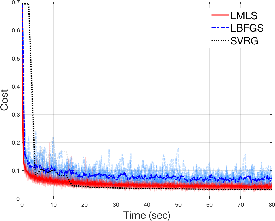
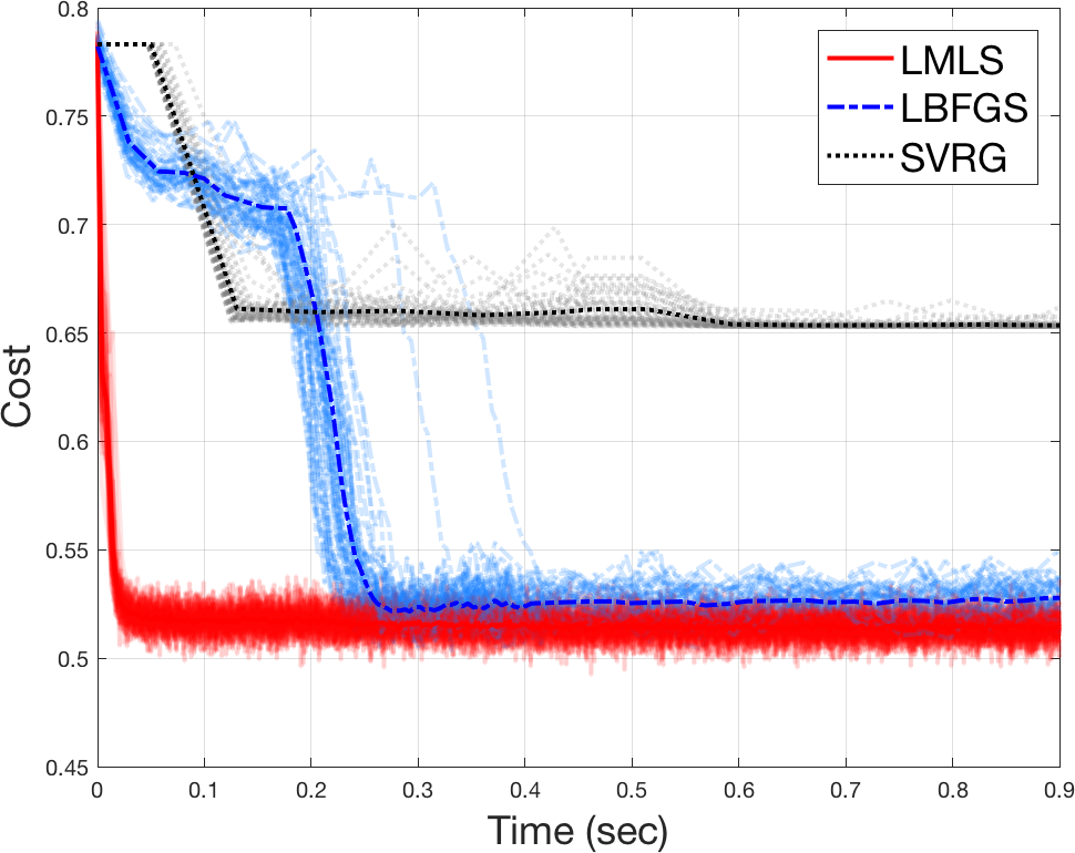
We compared our limited memory least-squares approach (denoted as LMLS) against two existing methods from the literature, namely, the limited memory stochastic BFGS method after Bollapragada et al. 2018 (denoted as LBFGS) and the stochastic variance reduced gradient descent (SVRG) by Johnson & Zhang 2013 (denoted SVRG). Figures 1(a) and 1(b) show the cost versus time for $50$ Monte-Carlo experiments.

5.2 Deep learning

Deep convolutional neural networks (CNNs) with multiple layers of convolution, pooling and nonlinear activation functions are delivering state-of-the-art results on many tasks in computer vision. We are here borrowing the stochastic optimisation problems arising in using such a deep CNN to solve the MNIST and CIFAR-10 benchmarks. The particular CNN structure used for the MNIST example employs $5\times 5$ convolution kernels, pooling layers and a fully connected layer at the end. We made use of the publicly available code provided by Zhang 2016, which contains all the implementation details. For the CIFAR-10 example, the network includes 13-layers with more than 150,000 weights, see Appendix D for details. The Matlab toolbox MatConvNet (Vedaldi & Lenc 2015) was used in the implementation. Figures 1(c) and 1(d) show the average cost versus time for $10$ Monte-Carlo trials with four different algorithms: 1. the method developed here (LMLS), 2. a stochastic limited memory BFGS method after Bollapragada et al. 2018 (denoted LBFGS), 3. Adam developed by Kingma & Ba 2015, and 4. stochastic gradient (denoted SG). Note that all algorithms make use of the same gradient code.

6 Conclusion and future work

In this work we have presented a least-squares based limited memory optimisation routine that benefits from second order information by approximating the inverse Hessian matrix. The procedure is conceptually similar to quasi-Newton methods, although we do not explicitly enforce symmetry or satisfaction of the secant condition. By regularising with respect to an inverse Hessian prior, we allow for an adaptive aggressiveness in the search direction update. We have shown that the computations can be made robust and efficient using tailored Cholesky decompositions, with a cost that scales linearly in the problem dimension. Our method is designed for stochastic problems through a line search that repeatedly decreases the step length so as to satisfy the first Wolfe condition in expectation. Theoretical results have been established that support the proposed procedure. The method shows improved convergence properties over existing algorithms when applied to benchmark problems of various size and complexity.

References

Armijo (1966) L. Armijo. Minimization of functions having Lipschitz continuous first partial derivatives. Pacific Journal of Mathematics, 16(1):1–3, 1966.
Bollapragada et al. (2018) R. Bollapragada, D. Mudigere, J. Nocedal, H.-J. M. Shi, and P. T. P. Tang. A progressive batching L-BFGS method for machine learning. In Proceedings of the 35th International Conference on Machine Learning (ICML), Stockholm, Sweden, 2018.
Bordes et al. (2009) A. Bordes, L. Bottou, and P. Gallinari. SGD-QN: Careful quasi-Newton stochastic gradient descent. Journal of Machine Learning Research (JMLR), 10:1737–1754, 2009.
Bottou et al. (2018) L. Bottou, F. E. Curtis, and J. Nocedal. Optimization methods for large-scale machine learning. SIAM Review, 60(2):223–311, 2018.
Broyden (1967) C. G. Broyden. Quasi-Newton methods and their application to function minimization. Mathematics of Computation, 21:368–381, 1967.
Broyden (1970) C. G. Broyden. The convergence of a class of double-rank minimization algorithms. Journal of the Institute of Mathematics and Its Applications, 6(1):76–90, 1970.
Byrd et al. (2016) R. H. Byrd, S. L. Hansen, J. Nocedal, and Y. Singer. A stochastic quasi-Newton method for large-scale optimization. SIAM Journal on Optimization, 26(2):1008–1031, 2016.
Chang & Lin (2011) C.-C. Chang and C.-J. Lin. LIBSVM: A library for support vector machines. ACM Transactions on Intelligent Systems and Technology, 2(3):27:1–27:27, 2011.
Defazio et al. (2014) A. Defazio, F. Bach, and S. Lacoste-Julien. SAGA: a fast incremental gradient method with support for non-strongly convex composite objectives. In Advances in Neural Information Processing Systems (NIPS), Montréal, Canada, 2014.
Duchi et al. (2011) J. Duchi, E. Hazan, and Y. Singer. Adaptive subgradient methods for online learning and stochastic optimization. Journal of Machine Learning Research (JMLR), 12:2121–2159, 2011.
Fletcher (1970) R. Fletcher. A new approach to variable metric algorithms. The computer journal, 13(3):317–322, 1970.
Fletcher (1987) R. Fletcher. Practical methods of optimization. John Wiley & Sons, Chichester, UK, second edition, 1987.
Goldfarb (1970) D. Goldfarb. A family of variable metric updates derived by variational means. Mathematics of Computation, 24(109):23–26, 1970.
Golub & Van Loan (2012) G. H. Golub and C. F. Van Loan. Matrix Computations. John Hopkins University Press, Baltimore, fourth edition, 2012.
Gower et al. (2016) R. M. Gower, D. Goldfarb, and P. Richtarik. Stochastic block BFGS: squeezing more curvature out of data. In Proceedings of the 33rd International Conference on Machine Learning (ICML), New York, NY, USA, 2016.
Hennig (2015) P. Hennig. Probabilistic interpretation of linear solvers. SIAM Journal on Optimization, 25(1):234–260, 2015.
Johnson & Zhang (2013) R. Johnson and T. Zhang. Accelerating stochastic gradient descent using predictive variance reduction. In Advances in Neural Information Processing Systems (NIPS), Lake Tahoe, NV, USA, 2013.
Kingma & Ba (2015) D. P. Kingma and J. Ba. Adam: a method for stochastic optimization. In Proceedings of the 3rd international conference on learning representations (ICLR), San Diego, CA, USA, 2015.
Konečný & Richtárik (2017) J. Konečný and P. Richtárik. Semi-stochastic gradient descent methods. Frontiers in Applied Mathematics and Statistics, 3(9), 2017.
Krizhevsky (2009) Alex Krizhevsky. Learning multiple layers of features from tiny images. Technical report, 2009.
Liu & Nocedal (1989) D. C. Liu and J. Nocedal. On the limited memory BFGS method for large scale optimization. Mathematical Programming, 45(3):503–528, 1989.
Mahsereci & Hennig (2017) M. Mahsereci and P. Hennig. Probabilistic line searches for stochastic optimization. Journal of Machine Learning Research (JMLR), 18(119):1–59, 2017.
Mokhtari & Ribeiro (2014) A. Mokhtari and A. Ribeiro. RES: regularized stochastic BFGS algorithm. IEEE Transactions on Signal Processing, 62(23):6089–6104, 2014.
Mokhtari & Ribeiro (2015) A. Mokhtari and A. Ribeiro. Global convergence of online limited memory BFGS. Journal of Machine Learning Research (JMLR), 16:3151–3181, 2015.
Moritz et al. (2016) P. Moritz, R. Nishihara, and M. I. Jordan. A linearly-convergent stochastic L-BFGS algorithm. In The 19th International Conference on Artificial Intelligence and Statistics (AISTATS), Cadiz, Spain, 2016.
Nocedal (1980) J. Nocedal. Updating quasi-Newton matrices with limited storage. Mathematics of Computation, 35(151):773–782, 1980.
Nocedal & Wright (2006) J. Nocedal and S. J. Wright. Numerical Optimization. Springer Series in Operations Research. Springer, New York, USA, second edition, 2006.
Robbins & Monro (1951) H. Robbins and S. Monro. A stochastic approximation method. Annals of Mathematical Statistics, 22(3):400–407, 1951.
Schmidt et al. (2013) M. Schmidt, N. Le Roux, and F. Bach. Minimizing finite sums with the stochastic average gradient. Technical Report arXiv:1309.2388, arXiv preprint, 2013.
Schraudolph et al. (2007) N. N. Schraudolph, J. Yu, and S. Günter. A stochastic quasi-Newton method for online convex optimization. In Proceedings of the 11th international conference on Artificial Intelligence and Statistics (AISTATS), 2007.
Shanno (1970) D. F. Shanno. Conditioning of quasi-Newton methods for function minimization. Mathematics of Computation, 24(111):647–656, 1970.
Vedaldi & Lenc (2015) A. Vedaldi and K. Lenc. Matconvnet – convolutional neural networks for matlab. In Proceeding of the ACM Int. Conf. on Multimedia, 2015.
Wang et al. (2017) X. Wang, S. Ma, D. Goldfarb, and W. Liu. Stochastic quasi-Newton methods for nonconvex stochastic optimization. SIAM Journal on Optimization, 27(2):927–956, 2017.
Wolfe (1969) P. Wolfe. Convergence conditions for ascent methods. SIAM Review, 11(2):226–235, 1969.
Wolfe (1971) P. Wolfe. Convergence conditions for ascent methods II: some corrections. SIAM Review, 13(2):185–188, 1971.
Zhang (2016) Z. Zhang. Derivation of backpropagation in convolutional neural networks (CNN). github.com/ZZUTK/An-Example-of-CNN-on-MNIST-dataset, 2016.

Appendix A Proofs of the lemmas

A.1 The first stochastic Wolfe condition

In the interest of a simple notation we note that we can drop the sub-index $k$ from all variables since all reasoning in this proof is for iteration $k$ . We also drop $x$ from the arguments and write $f$ rather than $f(x)$ , etc. However, we do make the randomness explicit, since this is crucial for arriving at the correct answer. For example we write $\widehat{f}_{z}$ to indicate that the random variable $z$ was used in computing the estimate of the function value at the iterate $x_{k}$ . This means that the noise contaminating the measurement corresponds to the realisation of $z$ .

Consider the stochastic version of the Wolfe condition

\displaystyle\operatorname{E}_{z,z^{\prime}}\left[\widehat{f}_{z^{\prime}}(x+\alpha\widehat{p}_{z})-\widehat{f}_{z}(x)-c\alpha\widehat{p}^{\mathsf{T}}_{z}\widehat{g}_{z}\right]\leq 0,

(36)

where the expected value is w.r.t. the randomness used in computing the required estimators as indicated by $z$ and $z^{\prime}$ . Using Taylor series we can for small step lengths $\alpha$ express $\widehat{f}_{z^{\prime}}(x+\alpha\widehat{p}_{z})$ according to

\displaystyle\widehat{f}_{z^{\prime}}(x+\alpha\widehat{p}_{z})\approx\widehat{f}_{z^{\prime}}+\alpha\widehat{p}_{z}^{\mathsf{T}}\widehat{g}_{z^{\prime}}.

(37)

Here it is crucial to note that the randomness in the above estimate stem from two different sources. The search direction $\widehat{p}_{z}$ enters in the argument of the Taylor expansion which is why it has to be computed before actually performing the Taylor expansion, implying that the randomness is due to $z$ and not $z^{\prime}$ for the search direction. Based on equation 36 we have the following expression for the stochastic Wolfe condition

\displaystyle\operatorname{E}_{z,z^{\prime}}\left[\widehat{f}_{z^{\prime}}-\widehat{f}_{z}-\alpha\widehat{p}_{z}^{\mathsf{T}}\widehat{g}_{z^{\prime}}+c\alpha\widehat{p}_{z}^{\mathsf{T}}\widehat{g}_{z}\right]\leq 0.

(38)

Let $b$ denote a possible bias in the cost function estimator, then we have that $\operatorname{E}_{z^{\prime}}\left[\widehat{f}_{z^{\prime}}\right]=f+b$ and $\operatorname{E}_{z}\left[\widehat{f}_{z}\right]=f+b$ . Hence, the first two terms in equation 38 cancel and we have

\displaystyle c\leq\frac{\operatorname{E}_{z,z^{\prime}}\left[\widehat{p}_{z}^{\mathsf{T}}\widehat{g}_{z^{\prime}}\right]}{\operatorname{E}_{z,z^{\prime}}\left[\widehat{p}_{z}^{\mathsf{T}}\widehat{g}_{z}\right]}=\frac{\operatorname{E}_{z}\left[\widehat{p}_{z}^{\mathsf{T}}\right]\operatorname{E}_{z^{\prime}}\left[\widehat{g}_{z^{\prime}}\right]}{\operatorname{E}_{z}\left[\widehat{p}_{z}^{\mathsf{T}}\widehat{g}_{z}\right]}=\frac{p^{\mathsf{T}}g}{\operatorname{E}_{z}\left[\widehat{p}_{z}^{\mathsf{T}}\widehat{g}_{z}\right]}.

(39)

The denominator can be written as

\displaystyle\operatorname{E}_{z}\left[\widehat{p}_{z}^{\mathsf{T}}\widehat{g}_{z}\right]=\operatorname{E}_{z}\left[-\widehat{g}_{z}^{\mathsf{T}}H\widehat{g}_{z}\right]=-\operatorname{E}_{z}\left[\Tr\left(H\widehat{g}_{z}\widehat{g}_{z}^{\mathsf{T}}\right)\right]=-\Tr\left(H\operatorname{E}_{z}\left[\widehat{g}_{z}\widehat{g}_{z}^{\mathsf{T}}\right]\right).

(40)

Using the definition of covariance we have that

\displaystyle\operatorname{E}_{z}\left[\widehat{g}_{z}\widehat{g}_{z}^{\mathsf{T}}\right]=\operatorname{E}_{z}\left[\widehat{g}_{z}\right]\operatorname{E}_{z}\left[\widehat{g}_{z}^{\mathsf{T}}\right]+\mathrm{Cov}{\widehat{g}}=gg^{\mathsf{T}}+\sigma_{g}^{2}I,

(41)

where we in the last equality made use of the assumption that the gradients are unbiased and that $\mathrm{Cov}{\widehat{g}}=\sigma_{g}I$ . Summarising we have that

\displaystyle\operatorname{E}_{z}\left[\widehat{p}_{z}^{\mathsf{T}}\widehat{g}_{z}\right]=-\Tr\left(Hgg^{\mathsf{T}}\right)-\sigma_{g}^{2}\Tr\left(H\right)=p^{\mathsf{T}}g-\sigma_{g}^{2}\Tr\left(H\right),

(42)

and hence we get

\displaystyle c\leq\frac{p^{\mathsf{T}}g}{p^{\mathsf{T}}g-\sigma_{g}^{2}\Tr\left(H\right)}.

(43)

Recalling the assurance given in lemma 3 with the associated proof in Appendix A.3, we can always modify $p$ to guarantee that this bound is positive.

A.2 Reduction in cost function

In this section we show that there exists an $\alpha>0$ such that

\displaystyle\operatorname{E}_{z^{\prime}}\left[\widehat{f}_{z^{\prime}}(x+\alpha p)\right]<\operatorname{E}_{z}\left[\widehat{f}_{z}(x)\right].

(44)

We do this by studying the difference

\displaystyle\operatorname{E}_{z^{\prime}}\left[\widehat{f}_{z^{\prime}}(x+\alpha p)\right]-\operatorname{E}_{z}\left[\widehat{f}_{z}(x)\right]=\operatorname{E}_{z,z^{\prime}}\left[\widehat{f}_{z^{\prime}}(x+\alpha p)-\widehat{f}_{z}(x)\right],

(45)

in which the first term can be expressed using a Taylor series according to

\displaystyle\widehat{f}_{z^{\prime}}(x+\alpha\widehat{p}_{z})=\widehat{f}_{z^{\prime}}+\alpha\widehat{p}_{z}^{\mathsf{T}}\widehat{g}_{z^{\prime}}+\mathcal{O}(\alpha\|\widehat{p}_{z}\|^{2}).

(46)

For small values of $\alpha$ we can discard the term $\mathcal{O}(\alpha\|\widehat{p}_{z}\|^{2})$ from this expression. Hence we have that

\displaystyle\operatorname{E}_{z,z^{\prime}}\left[\widehat{f}_{z^{\prime}}+\alpha\widehat{p}_{z}^{\mathsf{T}}\widehat{g}_{z^{\prime}}-\widehat{f}_{z}\right]=\alpha\operatorname{E}_{z,z^{\prime}}\left[\widehat{p}_{z}^{\mathsf{T}}\widehat{g}_{z^{\prime}}\right]=\alpha\operatorname{E}_{z}\left[\widehat{p}_{z}^{\mathsf{T}}\right]\operatorname{E}_{z^{\prime}}\left[\widehat{g}_{z^{\prime}}\right]=\alpha p^{\mathsf{T}}g.

(47)

Following from Section 4 we can ensure $p^{\mathsf{T}}g$ to be negative, and hence equation 44 holds as long as $\alpha$ is chosen small enough for the Taylor expansion to be a valid approximation.

A.3 Ensuring a descent direction

Note that

\displaystyle\operatorname{E}_{z}\left[(\widehat{p}_{z}-\beta\widehat{g}_{z})^{\mathsf{T}}\widehat{g}_{z}\right]=\operatorname{E}_{z}\left[\widehat{p}_{z}^{\mathsf{T}}\widehat{g}_{z}\right]-\beta\operatorname{E}_{z}\left[\widehat{g}_{z}^{\mathsf{T}}\widehat{g}_{z}\right]=\operatorname{E}_{z}\left[-\widehat{g}_{z}^{\mathsf{T}}H\widehat{g}_{z}\right]-\beta\operatorname{E}_{z}\left[\widehat{g}_{z}^{\mathsf{T}}\widehat{g}_{z}\right].

(48)

Using equation 42 we have

\displaystyle\operatorname{E}_{z}\left[-\widehat{g}_{z}^{\mathsf{T}}H\widehat{g}_{z}\right]=-\Tr\left(Hgg^{\mathsf{T}}\right)-\sigma_{g}^{2}\Tr\left(H\right)=p^{\mathsf{T}}g-\sigma_{g}^{2}\Tr\left(H\right),

(49)

and it directly follows from this that

\displaystyle\operatorname{E}_{z}\left[\widehat{g}_{z}^{\mathsf{T}}\widehat{g}_{z}\right]

\displaystyle=\operatorname{E}_{z}\left[-\widehat{g}_{z}^{\mathsf{T}}I\widehat{g}_{z}\right]=g^{\mathsf{T}}g+d\sigma_{g}^{2}.

(50)

Hence

\displaystyle\operatorname{E}_{z}\left[(\widehat{p}_{z}-\beta\widehat{g}_{z})^{\mathsf{T}}\widehat{g}_{z}\right]=p^{\mathsf{T}}g-\sigma_{g}^{2}\Tr\left(H\right)-\beta\left(g^{\mathsf{T}}g+d\sigma_{g}^{2}\right),

(51)

and we see that

\displaystyle\operatorname{E}_{z}\left[(\widehat{p}_{z}-\beta\widehat{g}_{z})^{\mathsf{T}}\widehat{g}_{z}\right]<0\Leftrightarrow\beta>\frac{p^{\mathsf{T}}g-\sigma_{g}^{2}\Tr\left(H\right)}{g^{\mathsf{T}}g+d\sigma_{g}^{2}}.

(52)

Appendix B Quasi-Newton methods

The historically most popular quasi-Newton method is given by the BFGS algorithm (Broyden 1970; Fletcher 1970; Goldfarb 1970; Shanno 1970)

\displaystyle H_{k+1}=\left(I-\frac{s_{k}y_{k}^{\mathsf{T}}}{y_{k}^{\mathsf{T}}s_{k}}\right)H_{k}\left(I-\frac{y_{k}s_{k}^{\mathsf{T}}}{y_{k}^{\mathsf{T}}s_{k}}\right)+\frac{s_{k}s_{k}^{\mathsf{T}}}{y_{k}^{\mathsf{T}}s_{k}}.

(53)

A closely related version is obtained if the optimisation in equation 11 is done with respect to the Hessian matrix rather than to its inverse. This results in the so-called DFP formula

\displaystyle H_{k+1}=H_{k}-\frac{H_{k}y_{k}y_{k}^{\mathsf{T}}H_{k}}{y_{k}^{\mathsf{T}}H_{k}y_{k}}+\frac{s_{k}s_{k}^{\mathsf{T}}}{y_{k}^{\mathsf{T}}s_{k}}.

(54)

Both of these are rank 2 updates that ensure $H_{k}$ to be positive definite, an attractive feature in the sense that it guarantees a descent direction. However, it may cause problems in regions where the true inverse Hessian is indefinite. Another well-known alternative is the symmetric rank 1 (SR1) method

\displaystyle H_{k}=H_{k-1}+\frac{(s_{k}-H_{k-1}y_{k})(s_{k}-H_{k-1}y_{k})^{\mathsf{T}}}{(s_{k}-H_{k-1}y_{k})^{\mathsf{T}}y_{k}}.

(55)

Apart from BFGS and DFP above, this is a rank 1 update that in general does not preserve positive definiteness. For this reason it has received a particular interest within the so-called trust-region framework, where its ability of producing indefinite inverse Hessian approximations is being regarded as a major strength (Nocedal & Wright 2006).

A main drawback of quasi-Newton methods is that they scale poorly to large problems, since the number of elements in $H_{k}$ equals the square of the input dimension $d$ . This has resulted in developments of so-called limited memory algorithms, which rely upon the idea of forming the search direction $p_{k}$ directly without the need of storing the full matrix $H_{k}$ . To that end a number $m<<d$ of past differences $y$ and $s$ are being stored in memory. A notable member of this family is the L-BFGS algorithm (Nocedal 1980), which has been widely within large-scale optimisation. During recent years, not at least due to the growing number of deep learning applications, there has been an increasing interest in adapting deterministic limited memory methods to the stochastic setting (Wang et al. 2017; Moritz et al. 2016; Gower et al. 2016; Schraudolph et al. 2007; Bordes et al. 2009; Mokhtari & Ribeiro 2015; Byrd et al. 2016; Bollapragada et al. 2018).

Appendix C Resulting algorithm

We summarise our ideas from Section 3 and 4 in Algorithm 2. The if-statement on line 5 is included to provide a safe-guard against numerical instability.

Algorithm 2 Stochastic quasi-Newton with line search

0: An initial estimate

x_{1}

, a maximum number of iterations

k_{\max}

, memory limit

m

, regularisation parameter

\lambda

, scale factor

\rho\in(0,1)

, reduction limit

\xi\geq 1

, backtracking limit

\tau>0

1: Set

k=1

2: while

k<k_{\max}

3: Obtain a measurement of the cost function and its gradient


	$\displaystyle\widehat{f}_{k}$	$\displaystyle=f(x_{k})+e_{k},$
	$\displaystyle\widehat{g}_{k}$	$\displaystyle=g_{k}+v_{k}.$

4: Set

\bar{H}_{k}=\gamma_{k}I

where

\displaystyle\gamma_{k}=\begin{cases}\hskip-8.53581pt\begin{split}\kappa\gamma_{k-1},\qquad&\text{if }\alpha_{k-1}=1,\\ \gamma_{k-1}/\kappa,\qquad&\text{if }\alpha_{k-1}<1/\rho^{q},\\ \gamma_{k-1},\qquad&\text{otherwise}.\end{split}\end{cases}

5: if

\widehat{y}_{k}^{\mathsf{T}}s_{k}>\epsilon\|s_{k}\|_{2}^{2}

then

6: if

k>m

then

7: Form

Y_{k}

and

S_{k}

by replacing the oldest vector-pairs in

Y_{k-1}

and

S_{k-1}

with

\widehat{y}_{k}

and

s_{k}

8: else

9: Form

Y_{k}

and

S_{k}

by adding

\widehat{y}_{k}

and

s_{k}

Y_{k-1}

and

S_{k-1}

10: end if

11: else

12: Set

Y_{k}=Y_{k-1}

and

S_{k}=S_{k-1}

13: end if

14: Select

\widehat{p}_{k}

	$\displaystyle\widehat{p}_{k}$	$\displaystyle=-\bar{H}_{k}z_{k}-\lambda^{-1}S_{k}(Y_{k}^{\mathsf{T}}z_{k}),$
	$\displaystyle z_{k}$	$\displaystyle=\widehat{g}_{k}-Y_{k}w_{k},$
	$\displaystyle w_{k}$	$\displaystyle=R_{k}^{-1}\left(R_{k}^{-\mathsf{T}}\left(Y_{k}^{\mathsf{T}}\widehat{g}_{k}\right)\right),$

with details provided in Section 4.2.

15: Set

\widehat{p}_{k}\leftarrow\widehat{p}_{k}-\beta_{k}\widehat{g}_{k}

with

\beta_{k}

where

\displaystyle\beta_{k}>\frac{\widehat{p}_{k}^{\mathsf{T}}\widehat{g}_{k}-\widehat{\sigma_{g}^{2}}\Tr\left(H\right)}{\widehat{g}_{k}^{\mathsf{T}}\widehat{g}_{k}+d\widehat{\sigma_{g}^{2}}}.

16: Set

\alpha_{k}=\min\{1,\xi/k\}

17: Set

i=1

18: while

\widehat{f}(x_{k}+\alpha\widehat{p}_{k})>\widehat{f}(x_{k})+c\alpha_{k}\widehat{g}_{k}^{\mathsf{T}}\widehat{p}_{k}

and

i\leq\max\{0,\tau-k\}

19: Reduce the step length

\alpha_{k}\leftarrow\rho\alpha_{k}

20: Set

i\leftarrow i+1

21: end while

22: Update

x_{k+1}=x_{k}+\alpha_{k}\widehat{p}_{k}

23: Set

k\leftarrow k+1

24: end while

Appendix D Experiment details

Details for the datasets used in Section 5 are listed in Table 1, including the parameter choices we made in our algorithm. Here, $b$ denotes the mini-batch size. The results of all logistic regression experiments are collected in Figure 2 (including those already shown in Figure 1), and the neural network results in Figures 1(d) and 1(c) are provided in a more readable size in Figure 3(a) and 3(b). Detailed information of the network structure in the CIFAR experiment is provided in the printout shown in Figure 4.

The adaptive procedure of selecting the inverse Hessian prior $\bar{H}_{k}$ did not have much impact in most of the logistic regression examples, and thus it was kept constant $\bar{H}_{k}=\gamma_{0}I$ except for in the covtype and URL problems. In the CIFAR and MNIST problems, however, the procedure was found to be of significant importance.

Table 1: List of the datasets used in the experiments, where

n

denotes the size of the dataset (column 2) and

d

denotes the number of variables in the optimisation problem (column 3). The remaining columns list our design parameters, including the mini-batch size

b

Problem	$n$	$d$	$b$	$m$	$\lambda$	$\xi$	$\tau$	$\gamma_{0}$
gisette	$6\thinspace 000$	$5\thinspace 000$	$770$	$20$	$10^{-4}$	$50$	$10$	$10$
covtype	$581\thinspace 012$	$54$	$7\thinspace 620$	$55$	$10^{-4}$	$100$	$5$	$100$
HIGGS	$11\thinspace 000\thinspace 000$	$28$	$66\thinspace 340$	$28$	$10^{-4}$	$20$	$5$	$100$
SUSY	$3\thinspace 548\thinspace 466$	$18$	$5\thinspace 000$	$18$	$10^{-4}$	$50$	$10$	$100$
epsilon	$400\thinspace 000$	$2\thinspace 000$	$1\thinspace 000$	$20$	$10^{-4}$	$150$	$1$	$100$
rcv1	$20\thinspace 242$	$47\thinspace 236$	$710$	$10$	$10^{-4}$	$50$	$10$	$600$
URL	$2\thinspace 396\thinspace 130$	$3\thinspace 231\thinspace 961$	$1548$	$5$	$10^{-4}$	$200$	$50$	$100$
spam	82 970	823 470	$2048$	$2$	$10^{-4}$	$150$	$10$	$200$
MNIST	60 000	$3898$	$1000$	$50$	$8\cdot 10^{-4}$	$150$	$50$	$1$
CIFAR	50 000	$150\thinspace 000$	$200$	$20$	$10^{-2}$	$100$	$10$	$0.5$