跳到论文正文
W Papers独立论文阅读器 arXiv:1810.01245 论文正文 计算阅读时间 · 0%
引用这篇论文根据当前论文元数据生成,正式投稿前建议核对。


License: arXiv.org perpetual non-exclusive license
arXiv:1810.01245v1 [physics.comp-ph] 26 Sep 2018

An interior penalty discontinuous Galerkin approach for 3D incompressible Navier–Stokes equation for permeability estimation of porous media

Chen Liu Address: Rice University, Department of Computational and Applied Mathematics, 6100 Main Street, Houston, TX 77005, USA    Florian Frank Address: Friedrich-Alexander-Universität Erlangen-Nürnberg, Department Mathematik, Cauerstraße 11, 91058 Erlangen, Germany    Faruk O. Alpak Address: Rice University, Department of Computational and Applied Mathematics, 6100 Main Street, Houston, TX 77005, USA Address: Shell Technology Center, 3333 Highway 6 South, Houston, TX 77082, USA    Béatrice Rivière Email: riviere@rice.edu Address: Rice University, Department of Computational and Applied Mathematics, 6100 Main Street, Houston, TX 77005, USA Corresponding author: Corresponding author: Béatrice Rivière
Abstract

Permeability estimation of porous media from direct solving Navier–Stokes equation has a wide spectrum of applications in petroleum industry. In this paper, we utilize a pressure-correction projection algorithm in conjunction with the interior penalty discontinuous Galerkin scheme for space discretization to build an incompressible Navier–Stokes simulator and to use this simulator to calculate permeability of real rock sample. The proposed method is accurate, numerically robust, and exhibits the potential for tackling realistic problems.

Keywords: 
incompressible Navier–Stokes equation , interior penalty discontinuous Galerkin method , projection method , porous media

1 Introduction

In the past decades, digital rock physics (DRP) has undergone rapid development. The modern X-ray microtomography (micro-CT) creates cross-sections of small rock samples on micrometer to millimeter scale by means of X-rays, which subsequently can be used to construct high-resolution model domains by 3D imaging software. This technique provides geometry patterns of rock structure, cf. Figure 1. With the increasing availability of computational resources and developments in numerical algorithms for 3D image reconstruction of pore structures, the use of direct numerical simulation for computing effective properties of a porous medium is playing a key role in the understanding of flows and rock interactions and is complementing time-consuming high-cost laboratory measurements. In addition, compared with traditional empirical formula based estimations, direct numerical simulation methods provide more accurate results, which attract much attention in hydro-geophysics and petroleum engineering fields.

Refer to caption
Figure 1: A 256×256×256256\times 256\times 256 voxel sets describing the fluid space of porous matrices.

Estimating permeabilities of rock matrices by direct numerical simulation usually requires large-scale computing to solve incompressible Navier–Stokes equation on complicated computational domains. Therefore an efficient numerical scheme becomes significantly important. The classical approach of solving the saddle-point problem by solving simultaneously the momentum and continuity equations has been well studied [1, 2]. However, this approach is not amenable for large systems. After taking both numerical accuracy and computational efficiency into account and balancing all considerations, one preferred technique is to decouple the nonlinear reaction term from the pressure term by using projection algorithms [3]. The splitting preserves important properties such as incompressibility or consistency with the boundary data. The literature on projection algorithms coupled with continuous finite element methods is vast. We refer the reader to an overview of the splitting techniques in [4, 5].

Interior penalty discontinuous Galerkin (IPDG) methods form a popular class of accurate and robust numerical schemes for solving partial differential equations [6, 7], which are known to be very flexible and have several positive features: local construction of trial and test spaces; curved boundaries and inhomogeneous boundary conditions are naturally handled; a local mass conservation property and suitability for parallelization in the context of large-scale simulations in complex domains. Due to these advantages, IPDG methods are widely used in computational fluid dynamics (CFD), geomechanics, and porous medium simulations. Although, a lot of research has been done for developing stable and high-order accurate solvers for CFD, there are very few works in the literature on the application of IPDG methods to incompressible flows for large scale computing. The use of discontinuous elements is studied in a pressure-correction algorithm in [8] and in a velocity-correction projection algorithm in [9]. The paper [8] employs a modified upwind scheme for the reaction term and a discretization of the projection step that are different from the ones we propose in this paper.

The paper’s contribution to the field of pore scale flows is a numerical approach for computing permeabilities of porous media. The porous structure is obtained from micro-CT imaging of the rock sample. IPDG methods combined with a projection algorithm are used to discretized the incompressible Navier–Stokes equations. The nonlinear system is linearized by a Picard splitting and a div–div correction postprocessing technique ensures a solenoidal velocity field. From the computed velocity and pressure fields, averages pressure and flux on inflow and outflow faces are obtained. The proposed approach is validated on benchmark problems. Numerical experiments on real rock images show the robustness of this method for handling 3D large scale simulations on complex geometries.

Estimating effective properties of rocks, such as absolute permeability, is one important objective of DRP [10]. There are few papers on the estimation of permeabilities from real rocks. For instance, the work [11] uses lattice Boltzmann method (LBM) and finite difference method to solve the Stokes equations and to obtain permeabilities of rock samples. More recently, a comprehensive numerical study of various rock samples is provided in [12] where permeability values are estimated by various solvers including LBM, continuous finite element, finite volume and fast Fourier transforms. Comparisons with experimental values show in some cases significant discrepancies. In addition, digital values of permeabilities vary from solver to solver. While the study does not fully address the reasons behind the mismatch, it highlights the need for accurate flow solvers. To our knowledge, this paper is the first to propose a DG-based solver for computing effective rock properties.

The outline of this paper follows. The incompressible Navier–Stokes model including boundary conditions for inflow, outflow, and fluid–solid interface are described in Section 2. The numerical algorithm is provided in Section 3. The validation tests and the numerical simulations for permeability estimation are given in Section 4.

2 Model Problem

Complex fluid phenomena in nature and in industrial applications give rise to a large number of challenging mathematical problems. The Navier–Stokes equations are the classical mathematical equations describing viscous gas and liquid flow. In this section, we introduce the equations for incompressible fluids, discuss the boundary conditions, and nondimensionalize the system equations.

2.1 Governing equations

Let Ω⊂ℝ3\Omega\subset\mathds{R}^{3} denote an open bounded polyhedral domain and let 𝒏{\boldsymbol{n}} denote the unit outer normal of Ω\Omega. Consider an incompressible fluid occupying the spatial domain Ω\Omega over the time interval (0,T)(0,T), where the unknown variables velocity 𝒗{\boldsymbol{v}} and pressure pp satisfy the Navier–Stokes equations:

ρ0​(∂t𝒗+𝒗⋅∇𝒗)−μs​Δ​𝒗\displaystyle\rho_{0}\,(\partial_{t}{{\boldsymbol{v}}}+{\boldsymbol{v}}\cdot{\boldsymbol{\nabla}}{{\boldsymbol{v}}})-\mu_{\mathrm{s}}\Delta{{\boldsymbol{v}}}~ =−∇p\displaystyle=~-{\boldsymbol{\nabla}}{p} in​(0,T)×Ω,\displaystyle\text{in}~(0,\,T)\times\Omega~, (1a)
∇⋅𝒗\displaystyle{\boldsymbol{\nabla}}\cdot{\boldsymbol{v}}~ =0\displaystyle=~0 in​(0,T)×Ω.\displaystyle\text{in}~(0,\,T)\times\Omega~. (1b)

Here, we assume a positive constant fluid density ρ0\rho_{0} and a positive constant shear viscosity μs\mu_{\mathrm{s}}. The diffusion term −Δ​𝒗-\Delta{{\boldsymbol{v}}} and the convection term 𝒗⋅∇𝒗{\boldsymbol{v}}\cdot{\boldsymbol{\nabla}}{{\boldsymbol{v}}} in eq. 1a are simplifications of the more general forms −2∇⋅𝜺(𝒗)-2{\boldsymbol{\nabla}}\cdot{{\boldsymbol{\varepsilon}}({\boldsymbol{v}})} and ∇⋅(𝒗⊗𝒗){\boldsymbol{\nabla}}\cdot{({\boldsymbol{v}}\otimes{\boldsymbol{v}})} , respectively, where

𝜺⁡(𝒗)=12​(∇𝒗+(∇𝒗)T){\boldsymbol{\varepsilon}}({\boldsymbol{v}})=\frac{1}{2}\big({\boldsymbol{\nabla}}{\boldsymbol{v}}+{({\boldsymbol{\nabla}}{\boldsymbol{v}})}^{\mathrm{T}}\big)

is the deformation tensor. The incompressibility constraint is expressed by eq. 1b, which is also called the pressure equation. With constraint eq. 1b, the equivalence of the diffusion and convection terms directly follows from the identities

2∇⋅𝜺(𝒗)\displaystyle 2{\boldsymbol{\nabla}}\cdot{{\boldsymbol{\varepsilon}}({\boldsymbol{v}})}~ =∇(∇⋅𝒗)+Δ​𝒗,\displaystyle=~{\boldsymbol{\nabla}}{({\boldsymbol{\nabla}}\cdot{{\boldsymbol{v}}})}+\Delta{{\boldsymbol{v}}}~,
∇⋅(𝒗⊗𝒗)\displaystyle{\boldsymbol{\nabla}}\cdot({\boldsymbol{v}}\otimes{\boldsymbol{v}})~ =𝒗⋅∇𝒗+(∇⋅𝒗)​𝒗.\displaystyle=~{\boldsymbol{v}}\cdot{\boldsymbol{\nabla}}{{\boldsymbol{v}}}+({\boldsymbol{\nabla}}\cdot{{\boldsymbol{v}}}){\boldsymbol{v}}~.

Note since these operators are mathematically equivalent in the model, one might consider formulating problems more generally. Even though these terms are identical, they lead to different boundary conditions. It turns out that using the more general expressions leads to unexpected behaviors of the velocity field at the outflow boundary in open boundary simulations, cf. Section 2.2.

2.2 Initial and boundary conditions

Boundary conditions play an important role in modeling various physical phenomena. In this section, we will consider two different scenarios, i. e., a closed boundary model and an open boundary model. For the former case, fluid flow across the boundary of the domain is suppressed. In both cases, eq. 1 is supplemented by the initial condition:

𝒗=𝒗0\displaystyle{\boldsymbol{v}}~=~{\boldsymbol{v}}^{0} on​{0}×Ω.\displaystyle\text{on}~\{0\}\times\Omega~. (2)

Closed boundary model

In this scenario, we assume the domain Ω\Omega is surrounded by a solid wall, i. e., ∂Ω=∂Ωwall\partial\Omega=\partial\Omega^{\mathrm{wall}}, where ∂Ωwall\partial\Omega^{\mathrm{wall}} denotes the fluid–solid interface. We employ the no-slip boundary condition (homogeneous Dirichlet condition):

𝒗=𝟎\displaystyle{\boldsymbol{v}}~=~{\boldsymbol{0}} on​(0,T)×∂Ω.\displaystyle\text{on}~(0,\,T)\times\partial\Omega~. (3)

Due to the boundary condition eq. 3, the pressure pp is uniquely defined up to an additive constant. To close this system, we also assume that the mean pressure in Ω\Omega equals zero:

∫Ωp=0.\int_{\Omega}p~=~0~. (4)

Benefitting from boundary condition eq. 3, the closed boundary Navier–Stokes model is an energy dissipative system. For regular enough solutions, a brief proof as follows.

Proposition 2.1.

The kinetic energy of system of problem {(1),(2),(3),(4)}\{\eqref{eq:GoverningEquationsNS},\eqref{eq:NS:IC},\eqref{eq:NS:closed_boundary_model_BC},\eqref{eq:NS:close_system_mean_p}\} is non-increasing in time, i. e., we have the identity, for all t∈(0,T)t\in(0,\,T):

dd​t∫Ω12ρ0|𝒗|2=−∫Ωμs∇𝒗:∇𝒗≤0.\frac{\mathrm{d}}{\mathrm{d}t}\int_{\Omega}\frac{1}{2}\rho_{0}|{\boldsymbol{v}}|^{2}~=~-\int_{\Omega}\mu_{\mathrm{s}}{\boldsymbol{\nabla}}{{\boldsymbol{v}}}:{\boldsymbol{\nabla}}{{\boldsymbol{v}}}~\leq~0~. (5)
Proof.

Taking the time derivative, based on the assumptions that the order of differentiation and integration can be changed, and by chain rule, we have pointwise in tt:

dd​t​∫Ω12​ρ0​|𝒗|2=∫Ω∂∂t​(12​ρ0​|𝒗|2)=∫Ω𝒗⋅(ρ0​∂t𝒗).\frac{\mathrm{d}}{\mathrm{d}t}\int_{\Omega}\frac{1}{2}\rho_{0}|{\boldsymbol{v}}|^{2}~=~\int_{\Omega}\frac{\partial}{\partial t}\Big(\frac{1}{2}\rho_{0}|{\boldsymbol{v}}|^{2}\Big)~=~\int_{\Omega}{\boldsymbol{v}}\cdot(\rho_{0}\partial_{t}{\boldsymbol{v}})~.

By eq. 1a, it follows

dd​t∫Ω12ρ0|𝒗|2=∫Ω−ρ0𝒗⋅(𝒗⋅∇𝒗)+∫Ωμs𝒗⋅Δ𝒗−∫Ω𝒗⋅∇p.\frac{\mathrm{d}}{\mathrm{d}t}\int_{\Omega}\frac{1}{2}\rho_{0}|{\boldsymbol{v}}|^{2}~=~\int_{\Omega}-\rho_{0}{\boldsymbol{v}}\cdot({\boldsymbol{v}}\cdot{\boldsymbol{\nabla}}{{\boldsymbol{v}}})+\int_{\Omega}\mu_{\mathrm{s}}{\boldsymbol{v}}\cdot\Delta{{\boldsymbol{v}}}-\int_{\Omega}{\boldsymbol{v}}\cdot{\boldsymbol{\nabla}}{p}~.

Using the incompressibility constraint eq. 1b and the boundary condition eq. 3, the following identities imply eq. 5

∫Ω𝒗⋅(𝒗⋅∇𝒗)\displaystyle\int_{\Omega}{\boldsymbol{v}}\cdot({\boldsymbol{v}}\cdot{\boldsymbol{\nabla}}{{\boldsymbol{v}}})~ =∫Ω(12𝒗⋅∇(𝒗⋅𝒗)−𝒗⋅(𝒗×∇×𝒗))\displaystyle=~\int_{\Omega}\Big(\frac{1}{2}{\boldsymbol{v}}\cdot{\boldsymbol{\nabla}}{({\boldsymbol{v}}\cdot{\boldsymbol{v}})}-{\boldsymbol{v}}\cdot({\boldsymbol{v}}\times{\boldsymbol{\nabla}}\times{{\boldsymbol{v}}})\Big)
=12∫Ω(−|𝒗|2∇⋅𝒗+∇⋅(|𝒗|2𝒗))=12∫∂Ω|𝒗|2𝒗⋅𝒏=0,\displaystyle=~\frac{1}{2}\int_{\Omega}\Big(-|{\boldsymbol{v}}|^{2}{\boldsymbol{\nabla}}\cdot{{\boldsymbol{v}}}+{\boldsymbol{\nabla}}\cdot{(|{\boldsymbol{v}}|^{2}{\boldsymbol{v}})}\Big)~=~\frac{1}{2}\int_{\partial\Omega}|{\boldsymbol{v}}|^{2}{\boldsymbol{v}}\cdot{\boldsymbol{n}}~=~0~,
∫Ω𝒗⋅Δ​𝒗\displaystyle\int_{\Omega}{\boldsymbol{v}}\cdot\Delta{{\boldsymbol{v}}}~ =∑i=1d∫ΩviΔvi=∑i=1d∫Ω(−∇vi⋅∇vi+∇⋅(vi∇vi))\displaystyle=~\sum_{i=1}^{d}\int_{\Omega}v^{i}\Delta{v^{i}}~=~\sum_{i=1}^{d}\int_{\Omega}\Big(-{\boldsymbol{\nabla}}{v^{i}}\cdot{\boldsymbol{\nabla}}{v^{i}}+{\boldsymbol{\nabla}}\cdot{(v^{i}{\boldsymbol{\nabla}}{v^{i}})}\Big)
=−∑i=1d∫Ω|∇vi|2+∑i=1d∫∂Ωvi∇vi⋅𝒏=−∫Ω∇𝒗:∇𝒗,\displaystyle=~-\sum_{i=1}^{d}\int_{\Omega}|{\boldsymbol{\nabla}}{v^{i}}|^{2}+\sum_{i=1}^{d}\int_{\partial\Omega}v^{i}{\boldsymbol{\nabla}}{v^{i}}\cdot{\boldsymbol{n}}~=~-\int_{\Omega}{\boldsymbol{\nabla}}{{\boldsymbol{v}}}:{\boldsymbol{\nabla}}{{\boldsymbol{v}}}~,
∫Ω𝒗⋅∇p\displaystyle\int_{\Omega}{\boldsymbol{v}}\cdot{\boldsymbol{\nabla}}{p}~ =∫Ω(−p∇⋅𝒗+∇⋅(p𝒗))=∫∂Ωp𝒗⋅𝒏=0.\displaystyle=~\int_{\Omega}\Big(-p{\boldsymbol{\nabla}}\cdot{{\boldsymbol{v}}}+{\boldsymbol{\nabla}}\cdot{(p{\boldsymbol{v}})}\Big)~=~\int_{\partial\Omega}p{\boldsymbol{v}}\cdot{\boldsymbol{n}}~=~0~.

∎

The energy dissipation law still holds in case of changing the diffusion term −μs​Δ​𝒗-\mu_{\mathrm{s}}\Delta{{\boldsymbol{v}}} in eq. 1a to −2∇⋅(μs𝜺(𝒗))-2{\boldsymbol{\nabla}}\cdot\big(\mu_{\mathrm{s}}{\boldsymbol{\varepsilon}}({\boldsymbol{v}})\big) . The modification of the proof can be easily obtained by using the tensor identity

∇⋅(μs​𝜺​(𝒗)​𝒗)=μs​𝜺​(𝒗):𝜺⁡(𝒗)+∇⋅(μs​𝜺​(𝒗))⋅𝒗,{\boldsymbol{\nabla}}\cdot{\big(\mu_{\mathrm{s}}{\boldsymbol{\varepsilon}}({\boldsymbol{v}}){\boldsymbol{v}}\big)}~=~\mu_{\mathrm{s}}\,{\boldsymbol{\varepsilon}}({\boldsymbol{v}}):{\boldsymbol{\varepsilon}}({\boldsymbol{v}})+{\boldsymbol{\nabla}}\cdot{\big(\mu_{\mathrm{s}}{\boldsymbol{\varepsilon}}({\boldsymbol{v}})\big)}\cdot{\boldsymbol{v}}~,

Note here, in this general case, μs\mu_{\mathrm{s}} may vary in space.

Open boundary model

In addition to the impervious fluid–solid interface ∂Ωwall\partial\Omega^{\mathrm{wall}}, we partition ∂Ω\partial\Omega into the inflow boundary and outflow boundary, which are defined as follows:

∂Ωin\displaystyle\partial\Omega^{\mathrm{in}}~ ={𝒙∈∂Ω:𝒗⋅𝒏<0},\displaystyle=~\{{\boldsymbol{x}}\in\partial\Omega:~{\boldsymbol{v}}\cdot{\boldsymbol{n}}~<~0\}~,
∂Ωout\displaystyle\partial\Omega^{\mathrm{out}}~ =∂Ω∖(∂Ωin∪∂Ωwall).\displaystyle=~\partial\Omega\setminus(\partial\Omega^{\mathrm{in}}\cup\partial\Omega^{\mathrm{wall}})~.

The fluid enters the domain Ω\Omega through ∂Ωin\partial\Omega^{\mathrm{in}} and exits through ∂Ωout\partial\Omega^{\mathrm{out}}. The unit normal vector, 𝒏{\boldsymbol{n}}, is outward to Ω\Omega. In this model, we prescribe inhomogeneous Dirichlet boundary condition on the inflow boundary, no-slip condition at the fluid–rock interface, and a Neumann-type condition on the outflow boundary

𝒗\displaystyle{\boldsymbol{v}}~ =𝒗in\displaystyle=~{\boldsymbol{v}}^{\mathrm{in}} on​(0,T)×∂Ωin,\displaystyle\text{on}~(0,\,T)\times\partial\Omega^{\mathrm{in}}~, (6a)
𝒗\displaystyle{\boldsymbol{v}}~ =𝟎\displaystyle=~{\boldsymbol{0}} on​(0,T)×∂Ωwall,\displaystyle\text{on}~(0,\,T)\times\partial\Omega^{\mathrm{wall}}~, (6b)
μs∇𝒗𝒏−p𝒏\displaystyle\mu_{\mathrm{s}}{\boldsymbol{\nabla}}{{\boldsymbol{v}}}\,{\boldsymbol{n}}-p\,{\boldsymbol{n}}~ =𝟎\displaystyle=~{\boldsymbol{0}} on​(0,T)×∂Ωout.\displaystyle\text{on}~(0,\,T)\times\partial\Omega^{\mathrm{out}}~. (6c)

Due to the fact that both eq. 6a and eq. 6b are Dirichlet-type conditions, we define

∂ΩD=∂Ωin∪∂Ωwall.\partial\Omega^{\mathrm{D}}~=~\partial\Omega^{\mathrm{in}}\cup\partial\Omega^{\mathrm{wall}}~.

In addition, we define 𝒗D{\boldsymbol{v}}_{\mathrm{D}} on ∂Ωin\partial\Omega^{\mathrm{in}} equal 𝒗in{\boldsymbol{v}}^{\mathrm{in}} and extend 𝒗D{\boldsymbol{v}}_{\mathrm{D}} on ∂Ωwall\partial\Omega^{\mathrm{wall}} by 𝟎{\boldsymbol{0}}. The condition on ∂Ωout\partial\Omega^{\mathrm{out}} is also called the open boundary condition. The motivation of introducing eq. 6c is that it enables us to simulate on a bounded computational domain to obtain the results identical to the case of fluid flow over unbounded or a relatively large region. Details for deriving eq. 6c are provided in [13] and this condition has been verified to be well-suited in modeling parallel flows [14].

The open boundary condition implies a zero mean pressure over outflow boundaries, which may cause undesirable effects within the flow region if more than one outlet exists [15]. Another alternative is to use the diffusion term −2∇⋅(μs𝜺(𝒗))-2{\boldsymbol{\nabla}}\cdot\big(\mu_{\mathrm{s}}{\boldsymbol{\varepsilon}}({\boldsymbol{v}})\big) instead of −μs​Δ​𝒗-\mu_{\mathrm{s}}\Delta{{\boldsymbol{v}}} in eq. 1a. Then, the boundary condition eq. 6c has to be modified to

2​μs​𝜺​(𝒗)​𝒏−p​𝒏=𝟎\displaystyle 2\mu_{\mathrm{s}}{\boldsymbol{\varepsilon}}{({\boldsymbol{v}})}\,{\boldsymbol{n}}-p\,{\boldsymbol{n}}~=~{\boldsymbol{0}} on (0,T)×∂Ωout.\displaystyle~(0,\,T)\times\partial\Omega^{\mathrm{out}}~.

Unfortunately, that choice leads to streamlines spreading outward at the outlet. Figure 2 shows Poiseuille flow in a cylinder for two choices of diffusion operators. In the left figure, the operator −μs​Δ​𝒗-\mu_{\mathrm{s}}\Delta{{\boldsymbol{v}}} is employed and in the right figure, the operator −2∇⋅(μs𝜺(𝒗))-2{\boldsymbol{\nabla}}\cdot\big(\mu_{\mathrm{s}}{\boldsymbol{\varepsilon}}({\boldsymbol{v}})\big) is used. We observe unphysical streamlines at the outflow boundary for the right figure.

Refer to caption Refer to caption
Figure 2: Left: open boundary cylindrical simulation with diffusion term −μs​Δ​𝒗-\mu_{\mathrm{s}}\Delta{{\boldsymbol{v}}}. Right: unphysical phenomenon of using deformation tensor −2∇⋅(μs𝜺(𝒗))-2{\boldsymbol{\nabla}}\cdot\big(\mu_{\mathrm{s}}{\boldsymbol{\varepsilon}}({\boldsymbol{v}})\big).

Throughout this paper, we focus on problems which are defined on channels with only one outlet and governed by eq. 1. Thus we avoid these drawbacks.

2.3 Nondimensionalization

The nondimensionalization process removes physical dimensions from the fluid mechanics model while producing dimensionless parameters which govern a whole family of dynamically similar flows. An advantage of analyzing problems in nondimensional form is the reduction of parameters. A brief review of the physical quantities and their units in the Navier–Stokes model is provided in Table 1.

Quantity Symbol Unit   | Quantity Symbol Unit
time tt s\mathrm{s}   | length xx m\mathrm{m}
velocity 𝒗{\boldsymbol{v}} m​s−1\mathrm{m}\,\mathrm{s}^{-1}   | pressure pp kg​m−1​s−2\mathrm{kg}\,\mathrm{m}^{-1}\,\mathrm{s}^{-2}
mass density ρ0\rho_{0} kg​m−3\mathrm{kg}\,\mathrm{m}^{-3}   | shear viscosity μs\mu_{\mathrm{s}} kg​m−1​s−1\mathrm{kg\,m^{-1}\,s^{-1}}
Table 1: Physical quantities used in the Navier–Stokes model and its units.

Let xcx_{\mathrm{c}} denote the characteristic length, tct_{\mathrm{c}} denote the characteristic time, vcv_{\mathrm{c}} denote the characteristic velocity, and pcp_{\mathrm{c}} denote the characteristic pressure, respectively. For simplicity, we still employ the same symbols for dimensionless quantities. With the choice tc=xc/vct_{\mathrm{c}}=x_{\mathrm{c}}/v_{\mathrm{c}} , the dimensionless version of eq. 1 becomes

∂t𝒗+𝒗⋅∇𝒗−1Re​Δ​𝒗\displaystyle\partial_{t}{\boldsymbol{v}}+{\boldsymbol{v}}\cdot{\boldsymbol{\nabla}}{{\boldsymbol{v}}}-\frac{1}{\mathrm{Re}}\Delta{{\boldsymbol{v}}}~ =−1X∇p\displaystyle=~-\frac{1}{\mathrm{X}}{\boldsymbol{\nabla}}{p} in​(0,T)×Ω,\displaystyle\text{in}~(0,\,T)\times\Omega~, (7a)
∇⋅𝒗\displaystyle{\boldsymbol{\nabla}}\cdot{\boldsymbol{v}}~ =0\displaystyle=~0 in​(0,T)×Ω,\displaystyle\text{in}~(0,\,T)\times\Omega~, (7b)
coupled with the initial and boundary conditions of the open boundary model in Section 2.2:
𝒗\displaystyle{\boldsymbol{v}}~ =𝒗0\displaystyle=~{\boldsymbol{v}}^{0} on​{0}×Ω,\displaystyle\text{on}~\{0\}\times\Omega~, (7c)
𝒗\displaystyle{\boldsymbol{v}}~ =𝒗in\displaystyle=~{\boldsymbol{v}}^{\mathrm{in}} on​(0,T)×∂Ωin,\displaystyle\text{on}~(0,\,T)\times\partial\Omega^{\mathrm{in}}~, (7d)
𝒗\displaystyle{\boldsymbol{v}}~ =𝟎\displaystyle=~{\boldsymbol{0}} on​(0,T)×∂Ωwall,\displaystyle\text{on}~(0,\,T)\times\partial\Omega^{\mathrm{wall}}~, (7e)
∇𝒗𝒏−ReXp𝒏\displaystyle{\boldsymbol{\nabla}}{{\boldsymbol{v}}}\,{\boldsymbol{n}}-\frac{\mathrm{Re}}{\mathrm{X}}p\,{\boldsymbol{n}}~ =𝟎\displaystyle=~{\boldsymbol{0}} on​(0,T)×∂Ωout.\displaystyle\text{on}~(0,\,T)\times\partial\Omega^{\mathrm{out}}~. (7f)

In eq. 7, Re\mathrm{Re} denotes the Reynolds number. We have:

Re=ρ0​vc​xcμs=ρ0​vc2μs​vc/xc,\mathrm{Re}~=~\frac{\rho_{0}\,v_{\mathrm{c}}\,x_{\mathrm{c}}}{\mu_{\mathrm{s}}}~=~\frac{\rho_{0}\,v_{\mathrm{c}}^{2}}{\mu_{\mathrm{s}}\,v_{\mathrm{c}}/x_{\mathrm{c}}}~,

which means that the Reynolds number expresses the ratio of inertia to viscous forces. The other dimensionless parameter in eq. 7 is

X=ρ0​vc2pc.\mathrm{X}~=~\frac{\rho_{0}\,v_{\mathrm{c}}^{2}}{p_{\mathrm{c}}}~.

3 Numerical Scheme

Direct numerical simulation of fluid flow in porous media needs to solve the time-dependent highly nonlinear Navier–Stokes equations. For this reason, we carefully design a numerical method to solve this system on large complex domains by taking both numerical accuracy and computational efficiency into account.

3.1 Preliminaries

Domain and triangulation

Let ℰh={Ek}\mathcal{E}_{h}=\{E_{k}\} be a family of conforming non-degenerate (also called regular) meshes of the domain Ω\Omega. The parameter hh denotes the maximum element diameter. Let Γh\Gamma_{h} donate the set of interior faces. For each interior face e∈Γhe\in\Gamma_{h} shared by elements Ek−E_{k^{-}} and Ek+E_{k^{+}}, we define a unit normal vector 𝒏e{\boldsymbol{n}}_{e} points from Ek−E_{k^{-}} into Ek+E_{k^{+}}. For the face ee on boundary ∂Ω\partial\Omega, i. e., e=Ek−∩∂Ωe=E_{k^{-}}\cap\partial\Omega, the normal 𝒏e{\boldsymbol{n}}_{e} is taken to be the unit outward vector to ∂Ω\partial\Omega.

We denote by ℙ1​(E)\mathds{P}_{1}(E) the set of linear polynomials on element EE and we define

ℙ1​(ℰh)=∏Ek∈ℰhℙ1​(Ek).\displaystyle\mathds{P}_{1}(\mathcal{E}_{h})~=~\prod_{E_{k}\in\mathcal{E}_{h}}\mathds{P}_{1}(E_{k})~.

The average and jump operator for any vector quantity 𝒗{\boldsymbol{v}} belonging to ℙ1​(ℰh)3\mathds{P}_{1}(\mathcal{E}_{h})^{3} are defined by

{|𝒗|}={12​𝒗|Ek−+12​𝒗|Ek+if​e=Ek−∩Ek+𝒗|Ek−if​e=Ek−∩∂Ω},\displaystyle\{\hskip-1.79993pt|{{\boldsymbol{v}}}|\hskip-1.79993pt\}~=~\begin{Bmatrix}[l]\frac{1}{2}\left.{\boldsymbol{v}}\right|_{E_{k^{-}}}+\frac{1}{2}\left.{\boldsymbol{v}}\right|_{E_{k^{+}}}&\text{if}~e=E_{k^{-}}\cap E_{k^{+}}~\\ \left.{\boldsymbol{v}}\right|_{E_{k^{-}}}&\text{if}~e=E_{k^{-}}\cap\partial\Omega~\end{Bmatrix}~, ⟦𝒗⟧={𝒗|Ek−−𝒗|Ek+if​e=Ek−∩Ek+𝒗|Ek−if​e=Ek−∩∂Ω}.\displaystyle\left\llbracket{{\boldsymbol{v}}}\right\rrbracket~=~\begin{Bmatrix}[l]\left.{\boldsymbol{v}}\right|_{E_{k^{-}}}-\left.{\boldsymbol{v}}\right|_{E_{k^{+}}}~~~~~~&\text{if}~e=E_{k^{-}}\cap E_{k^{+}}~\\ \left.{\boldsymbol{v}}\right|_{E_{k^{-}}}~~~~~~&\text{if}~e=E_{k^{-}}\cap\partial\Omega~\end{Bmatrix}~.

Note for scalar quantities, the jump and average definitions are similar.

DG forms

The DG discretization of the convection term 𝒗⋅∇𝒗{\boldsymbol{v}}\cdot{\boldsymbol{\nabla}}{{\boldsymbol{v}}} , the diffusion term −Δ​𝒗-\Delta{{\boldsymbol{v}}} , and the pressure term −∇p-{\boldsymbol{\nabla}}{p}, with the boundary conditions eq. 7, are

a𝒞​(𝒖,𝒛,𝜽)=−∑E∈ℰh∫E(𝒖⋅∇𝜽)⋅𝒛−12∑E∈ℰh∫E(∇⋅𝒖)𝒛⋅𝜽+∑e∈Γh∪∂Ωout∫e{|𝒖⋅𝒏e|}𝒛↑⋅⟦𝜽⟧+12∑e∈Γh∫e⟦𝒖⋅𝒏e⟧{|𝒛⋅𝜽|},\displaystyle\begin{split}a_{\mathcal{C}}({\boldsymbol{u}},{\boldsymbol{z}},{\boldsymbol{\theta}})~=~&-\sum_{E\in\mathcal{E}_{h}}\int_{E}({\boldsymbol{u}}\cdot{\boldsymbol{\nabla}}{\boldsymbol{\theta}})\cdot{\boldsymbol{z}}-\frac{1}{2}\sum_{E\in\mathcal{E}_{h}}\int_{E}({\boldsymbol{\nabla}}\cdot{{\boldsymbol{u}}})\,{\boldsymbol{z}}\cdot{{\boldsymbol{\theta}}}\\ &+\sum_{e\in\Gamma_{h}\cup\partial\Omega^{\mathrm{out}}}\int_{e}\{\hskip-1.79993pt|{{\boldsymbol{u}}\cdot{\boldsymbol{n}}_{e}}|\hskip-1.79993pt\}\,{\boldsymbol{z}}^{\uparrow}\cdot\left\llbracket{{\boldsymbol{\theta}}}\right\rrbracket+\frac{1}{2}\sum_{e\in\Gamma_{h}}\int_{e}\left\llbracket{{\boldsymbol{u}}\cdot{\boldsymbol{n}}_{e}}\right\rrbracket\{\hskip-1.79993pt|{{\boldsymbol{z}}\cdot{\boldsymbol{\theta}}}|\hskip-1.79993pt\}~,\end{split} (8a)
b𝒞​(𝜽)=\displaystyle b_{\mathcal{C}}({\boldsymbol{\theta}})~=~ −∑e∈∂Ωin∫e(𝒗D⋅𝒏)(𝒗D⋅𝜽),\displaystyle-\sum_{e\in\partial\Omega^{\mathrm{in}}}\int_{e}({\boldsymbol{v}}_{\mathrm{D}}\cdot{\boldsymbol{n}})({\boldsymbol{v}}_{\mathrm{D}}\cdot{\boldsymbol{\theta}})~, (8b)
a𝜺​(𝒗,𝜽)=∑E∈ℰh∫E∇𝒗:∇𝜽−∑e∈Γh∪∂ΩD∫e{|∇𝒗⋅𝒏e|}⋅⟦𝜽⟧+ϵ∑e∈Γh∪∂ΩD∫e{|∇𝜽⋅𝒏e|}⋅⟦𝒗⟧+σh∑e∈Γh∪∂ΩD∫e⟦𝒗⟧⋅⟦𝜽⟧,\displaystyle\begin{split}a_{\boldsymbol{\varepsilon}}({\boldsymbol{v}},{\boldsymbol{\theta}})~=~&\sum_{E\in\mathcal{E}_{h}}\int_{E}{\boldsymbol{\nabla}}{{\boldsymbol{v}}}:{\boldsymbol{\nabla}}{{\boldsymbol{\theta}}}-\sum_{e\in\Gamma_{h}\cup\partial\Omega^{\mathrm{D}}}\int_{e}\{\hskip-1.79993pt|{{\boldsymbol{\nabla}}{{\boldsymbol{v}}}\cdot{\boldsymbol{n}}_{e}}|\hskip-1.79993pt\}\cdot\left\llbracket{{\boldsymbol{\theta}}}\right\rrbracket\\ &+\epsilon\sum_{e\in\Gamma_{h}\cup\partial\Omega^{\mathrm{D}}}\int_{e}\{\hskip-1.79993pt|{{\boldsymbol{\nabla}}{{\boldsymbol{\theta}}}\cdot{\boldsymbol{n}}_{e}}|\hskip-1.79993pt\}\cdot\left\llbracket{{\boldsymbol{v}}}\right\rrbracket+\frac{\sigma}{h}\sum_{e\in\Gamma_{h}\cup\partial\Omega^{\mathrm{D}}}\int_{e}\left\llbracket{{\boldsymbol{v}}}\right\rrbracket\cdot\left\llbracket{{\boldsymbol{\theta}}}\right\rrbracket~,\end{split} (8c)
b𝜺​(𝜽)=\displaystyle b_{\boldsymbol{\varepsilon}}({\boldsymbol{\theta}})~=~ ϵ∑e∈∂ΩD∫e(∇𝜽⋅𝒏e)⋅𝒗D+σh∑e∈∂ΩD∫e𝒗D⋅𝜽,\displaystyle\epsilon\sum_{e\in\partial\Omega^{\mathrm{D}}}\int_{e}({\boldsymbol{\nabla}}{{\boldsymbol{\theta}}}\cdot{\boldsymbol{n}}_{e})\cdot{\boldsymbol{v}}_{\mathrm{D}}+\frac{\sigma}{h}\sum_{e\in\partial\Omega^{\mathrm{D}}}\int_{e}{\boldsymbol{v}}_{\mathrm{D}}\cdot{\boldsymbol{\theta}}~, (8d)
b𝒫​(p,𝜽)=\displaystyle b_{\mathcal{P}}(p,{\boldsymbol{\theta}})~=~ ∑E∈ℰh∫Ep∇⋅𝜽−∑e∈Γh∪∂ΩD∫e{|p|}⟦𝜽⋅𝒏e⟧.\displaystyle\sum_{E\in\mathcal{E}_{h}}\int_{E}p{\boldsymbol{\nabla}}\cdot{{\boldsymbol{\theta}}}-\sum_{e\in\Gamma_{h}\cup\partial\Omega^{\mathrm{D}}}\int_{e}\{\hskip-1.79993pt|{p}|\hskip-1.79993pt\}\left\llbracket{{\boldsymbol{\theta}}\cdot{\boldsymbol{n}}_{e}}\right\rrbracket~. (8e)
For the upwind flux in eq. 8a, we define the upwind quantity 𝒛↑{\boldsymbol{z}}^{\uparrow} of the vector quantity 𝒛{\boldsymbol{z}} on a face ee with normal 𝒏e=𝒏|Ek−{\boldsymbol{n}}_{e}=\left.{\boldsymbol{n}}\right|_{E_{k^{-}}} by
𝒛↑|e∈Γh={𝒛|Ek−if​{|𝒖|}⋅𝒏e≥0𝒛|Ek+if​{|𝒖|}⋅𝒏e<0}\displaystyle\left.{\boldsymbol{z}}^{\uparrow}\right|_{e\in\Gamma_{h}}=\begin{Bmatrix}[l]\left.{\boldsymbol{z}}\right|_{E_{k^{-}}}&\text{if}~\{\hskip-1.79993pt|{{\boldsymbol{u}}}|\hskip-1.79993pt\}\cdot{\boldsymbol{n}}_{e}\geq 0~\\ \left.{\boldsymbol{z}}\right|_{E_{k^{+}}}&\text{if}~\{\hskip-1.79993pt|{{\boldsymbol{u}}}|\hskip-1.79993pt\}\cdot{\boldsymbol{n}}_{e}<0~\end{Bmatrix} and 𝒛↑|e∈∂Ω={𝒛|Ek−if​𝒖⋅𝒏e≥0𝟎if​𝒖⋅𝒏e<0}.\displaystyle\left.{\boldsymbol{z}}^{\uparrow}\right|_{e\in\partial\Omega}=\begin{Bmatrix}[l]\left.{\boldsymbol{z}}\right|_{E_{k^{-}}}&\text{if}~{\boldsymbol{u}}\cdot{\boldsymbol{n}}_{e}\geq 0~\\ {\boldsymbol{0}}&\text{if}~{\boldsymbol{u}}\cdot{\boldsymbol{n}}_{e}<0~\end{Bmatrix}~.
In addition, the discretization of the elliptic operator −Δ​p-\Delta{p}, which will be employed in the pressure correction step, is
aellip​(p,χ)=∑E∈ℰh∫E∇p⋅∇χ−∑e∈Γh∪∂Ωout∫e{|∇p⋅𝒏e|}⟦χ⟧+ϵ∑e∈Γh∪∂Ωout∫e{|∇χ⋅𝒏e|}⟦p⟧+σh∑e∈Γh∪∂Ωout∫e⟦p⟧⟦χ⟧.\displaystyle\begin{split}a_{\mathrm{ellip}}(p,\chi)~=~&\sum_{E\in\mathcal{E}_{h}}\int_{E}{\boldsymbol{\nabla}}p\cdot{\boldsymbol{\nabla}}\chi-\sum_{e\in\Gamma_{h}\cup\partial\Omega^{\mathrm{out}}}\int_{e}\{\hskip-1.79993pt|{{\boldsymbol{\nabla}}p\cdot{\boldsymbol{n}}_{e}}|\hskip-1.79993pt\}\left\llbracket{\chi}\right\rrbracket\\ &+\epsilon\sum_{e\in\Gamma_{h}\cup\partial\Omega^{\mathrm{out}}}\int_{e}\{\hskip-1.79993pt|{{\boldsymbol{\nabla}}\chi\cdot{\boldsymbol{n}}_{e}}|\hskip-1.79993pt\}\left\llbracket{p}\right\rrbracket+\frac{\sigma}{h}\sum_{e\in\Gamma_{h}\cup\partial\Omega^{\mathrm{out}}}\int_{e}\left\llbracket{p}\right\rrbracket\left\llbracket{\chi}\right\rrbracket~.\end{split} (8f)

The choice of the parameter ϵ\epsilon in eqs. 8c, 8d and 8f yields the NIPG method (ϵ=1\epsilon=1) and the SIPG method (ϵ=−1\epsilon=-1). For NIPG method, the penalty parameter σ\sigma can be set to 11 and for SIPG method a large enough value is needed. A discussion about selecting the value of σ\sigma is provided in [16, 17]. For the derivation and properties of these DG forms, we refer to [6, 18] and the references herein.

3.2 Time discretization

In eq. 7, the velocity and pressure are coupled by the incompressibility constraint. The pressure-correction projection algorithm, which splits dynamics and incompressibility, is especially convenient for the large-scale three-dimensional numerical simulations. We now describe the splitting in time of the equations.

Uniformly partition [0,T][0,\,T] into NN subintervals and let τ\tau denote the time step length. For any 1≤n≤N1\leq n\leq N , given the solution at the previous time, (𝒗n−1,pn−1,ϕn−1)({\boldsymbol{v}}^{n-1},p^{n-1},\phi^{n-1}), the algorithm yields the solution at the current time in three steps. In the first velocity step, we employ Picard splitting to treat the nonlinear convection term and compute 𝒗n{\boldsymbol{v}}^{n} by solving the system:

𝒗n+τ​𝒗n−1⋅∇𝒗n−τRe​Δ​𝒗n\displaystyle{\boldsymbol{v}}^{n}+\tau{\boldsymbol{v}}^{n-1}\cdot{\boldsymbol{\nabla}}{{\boldsymbol{v}}^{n}}-\frac{\tau}{\mathrm{Re}}\Delta{{\boldsymbol{v}}^{n}}~ =𝒗n−1−τX∇(pn−1+ϕn−1)\displaystyle=~{\boldsymbol{v}}^{n-1}-\frac{\tau}{\mathrm{X}}{\boldsymbol{\nabla}}{(p^{n-1}+\phi^{n-1})} in​Ω,\displaystyle\text{in}~\Omega~, (9a)
𝒗n\displaystyle{\boldsymbol{v}}^{n}~ =𝒗in​(tn)\displaystyle=~{\boldsymbol{v}}^{\mathrm{in}}(t^{n}) on​∂Ωin,\displaystyle\text{on}~\partial\Omega^{\mathrm{in}}~, (9b)
𝒗n\displaystyle{\boldsymbol{v}}^{n}~ =𝟎\displaystyle=~{\boldsymbol{0}} on​∂Ωwall,\displaystyle\text{on}~\partial\Omega^{\mathrm{wall}}~, (9c)
∇𝒗n𝒏−ReXpn−1𝒏\displaystyle{\boldsymbol{\nabla}}{{\boldsymbol{v}}}^{n}{\boldsymbol{n}}-\frac{\mathrm{Re}}{\mathrm{X}}p^{n-1}\,{\boldsymbol{n}}~ =𝟎\displaystyle=~{\boldsymbol{0}} on​∂Ωout.\displaystyle\text{on}~\partial\Omega^{\mathrm{out}}~. (9d)

Then, in the pressure projection step, we solve a Poisson problem to compute the correction ϕn\phi^{n}:

−Δ​ϕn\displaystyle-\Delta{\phi^{n}}~ =−Xτ∇⋅𝒗n\displaystyle=~-\frac{\mathrm{X}}{\tau}{\boldsymbol{\nabla}}\cdot{{\boldsymbol{v}}^{n}} in​Ω,\displaystyle\text{in}~\Omega~, (10a)
∇ϕn⋅𝒏\displaystyle{\boldsymbol{\nabla}}{\phi^{n}}\cdot{\boldsymbol{n}}~ =0\displaystyle=~0 on​∂ΩD,\displaystyle\text{on}~\partial\Omega^{\mathrm{D}}~, (10b)
ϕn\displaystyle\phi^{n}~ =0\displaystyle=~0 on​∂Ωout.\displaystyle\text{on}~\partial\Omega^{\mathrm{out}}~. (10c)

Finally, in the postprocessing step, we update the pressure pnp^{n} and obtain a solenoidal velocity field 𝒖n{\boldsymbol{u}}^{n}:

pn\displaystyle p^{n}~ =pn−1+ϕn−XRe∇⋅𝒗n,\displaystyle=~p^{n-1}+\phi^{n}-\frac{\mathrm{X}}{\mathrm{Re}}\,{\boldsymbol{\nabla}}\cdot{{\boldsymbol{v}}^{n}}~, (11a)
𝒖n\displaystyle{\boldsymbol{u}}^{n}~ =𝒗n−τX∇ϕn.\displaystyle=~{\boldsymbol{v}}^{n}-\frac{\tau}{\mathrm{X}}\,{\boldsymbol{\nabla}}{\phi^{n}}~. (11b)

Here, for the initial condition, we set p0=0p^{0}=0 and ϕ0=0\phi^{0}=0. Note that both 𝒗n{\boldsymbol{v}}^{n} and 𝒖n{\boldsymbol{u}}^{n} are approximations of the velocity and 𝒗n{\boldsymbol{v}}^{n} satisfies the Dirichlet boundary condition while possibly violating an incompressibility constraint, whereas 𝒖n{\boldsymbol{u}}^{n} is solenoidal but satisfies the Dirichlet condition only in the normal direction.

3.3 Space discretization

Standard algorithm

We use IPDG method for spatial discretization for each of the three steps. The partition of the domain, DG operators, and related notation are introduced in Section 3.1. We also use the notation (⋅,⋅)(\cdot,\cdot) for the L2 inner-product on Ω\Omega.
The fully discrete scheme of the velocity step eq. 9 reads: for any 1≤n≤N1\leq n\leq N , find 𝒗hn∈ℙ1​(ℰh)3{\boldsymbol{v}}^{n}_{h}\in\mathds{P}_{1}(\mathcal{E}_{h})^{3} such that for all 𝜽h∈ℙ1​(ℰh)3{\boldsymbol{\theta}}_{h}\in\mathds{P}_{1}(\mathcal{E}_{h})^{3}:

(𝒗hn,𝜽h)+τ​a𝒞​(𝒗hn−1,𝒗hn,𝜽h)+τRe​a𝜺​(𝒗hn,𝜽h)=(𝒗hn−1,𝜽h)+τX​b𝒫​(phn−1,𝜽h)−τX​(∇ϕhn−1,𝜽h)+τ​b𝒞​(𝜽h)+τRe​b𝜺​(𝜽h).\displaystyle\begin{split}({\boldsymbol{v}}^{n}_{h},{\boldsymbol{\theta}}_{h})+\tau\,a_{\mathcal{C}}({\boldsymbol{v}}^{n-1}_{h},{\boldsymbol{v}}^{n}_{h},{\boldsymbol{\theta}}_{h})\,+&\,\frac{\tau}{\mathrm{Re}}a_{\boldsymbol{\varepsilon}}({\boldsymbol{v}}^{n}_{h},{\boldsymbol{\theta}}_{h})~=~({\boldsymbol{v}}^{n-1}_{h},{\boldsymbol{\theta}}_{h})\\ +&\,\frac{\tau}{\mathrm{X}}b_{\mathcal{P}}(p^{n-1}_{h},{\boldsymbol{\theta}}_{h})-\frac{\tau}{\mathrm{X}}({\boldsymbol{\nabla}}{\phi^{n-1}_{h}},{\boldsymbol{\theta}}_{h})+\tau b_{\mathcal{C}}({\boldsymbol{\theta}}_{h})+\frac{\tau}{\mathrm{Re}}b_{\boldsymbol{\varepsilon}}({\boldsymbol{\theta}}_{h})~.\end{split} (12)

For the pressure projection step eq. 10, the fully-discrete scheme is: for any 1≤n≤N1\leq n\leq N , find ϕhn∈ℙ1​(ℰh)\phi^{n}_{h}\in\mathds{P}_{1}(\mathcal{E}_{h}) such that for all χh∈ℙ1​(ℰh)\chi_{h}\in\mathds{P}_{1}(\mathcal{E}_{h}):

aellip​(ϕhn,χh)=−Xτ​(∇⋅𝒗hn,χh).\displaystyle a_{\mathrm{ellip}}(\phi^{n}_{h},\chi_{h})~=~-\frac{\mathrm{X}}{\tau}({\boldsymbol{\nabla}}\cdot{{\boldsymbol{v}}^{n}_{h}},\chi_{h})~. (13)

For the postprocessing step eq. 11, the discrete pressure and velocity are updated as follows: find phn∈ℙ1​(ℰh)p^{n}_{h}\in\mathds{P}_{1}(\mathcal{E}_{h}) and 𝒖hn∈ℙ1​(ℰh)3{\boldsymbol{u}}^{n}_{h}\in\mathds{P}_{1}(\mathcal{E}_{h})^{3} such that for all χh∈ℙ1​(ℰh)\chi_{h}\in\mathds{P}_{1}(\mathcal{E}_{h}) and 𝜽h∈ℙ1​(ℰh)3{\boldsymbol{\theta}}_{h}\in\mathds{P}_{1}(\mathcal{E}_{h})^{3}:

(phn,χh)\displaystyle(p^{n}_{h},\chi_{h})~ =(phn−1,χh)+(ϕhn,χh)−XRe​(∇⋅𝒗hn,χh),\displaystyle=~(p^{n-1}_{h},\chi_{h})+(\phi^{n}_{h},\chi_{h})-\frac{\mathrm{X}}{\mathrm{Re}}({\boldsymbol{\nabla}}\cdot{{\boldsymbol{v}}^{n}_{h}},\chi_{h})~, (14a)
(𝒖hn,𝜽h)\displaystyle({\boldsymbol{u}}^{n}_{h},{\boldsymbol{\theta}}_{h})~ =(𝒗hn,𝜽h)−τX​(∇ϕhn,𝜽h).\displaystyle=~({\boldsymbol{v}}^{n}_{h},{\boldsymbol{\theta}}_{h})-\frac{\tau}{\mathrm{X}}({\boldsymbol{\nabla}}{\phi^{n}_{h}},{\boldsymbol{\theta}}_{h})~. (14b)
The operator ∇{\boldsymbol{\nabla}}{} in eqs. 12 and 14b denotes the broken gradient, the operator ∇⁣⋅{\boldsymbol{\nabla}}\cdot{} in eqs. 13 and 14a denotes the broken divergence.
Remark 3.1.

We note that when ∂Ωin=∅\partial{\Omega}^{\mathrm{in}}=\emptyset and ∂Ωout=∅\partial{\Omega}^{\mathrm{out}}=\emptyset the open boundary system eq. 6 automatically degenerates to the closed boundary system with boundary condition in eq. 3. In this case, the time discretization in Section 3.2 is still effective except that we end up with a pure Neumann system for eq. 10, which means the linear system generated by eq. 13 will be singular. To overcome this challenge, the constraint in eq. 4 should be considered. We can introduce a Lagrange multiplier to produce an optimization problem and solve it. We omit technical details here, since this case is not our focus, and for those who are interested in this methodology, we refer to [19].

Div–div correction

It is worth to note that the standard algorithm may not provide a pointwise divergence free velocity field. A classical remedy is to apply the div–div stabilization technique [9]. The projection is stabilized by adding an additional term in eq. 14b. We employ the following form:

(𝒖hn,𝜽h)+σdiv​(∇⋅𝒖hn,∇⋅𝜽h)=(𝒗hn,𝜽h)−τX​(∇ϕhn,𝜽h),\displaystyle({\boldsymbol{u}}^{n}_{h},{\boldsymbol{\theta}}_{h})+\sigma_{\mathrm{div}}({\boldsymbol{\nabla}}\cdot{{\boldsymbol{u}}^{n}_{h}},{\boldsymbol{\nabla}}\cdot{{\boldsymbol{\theta}}_{h}})~=~({\boldsymbol{v}}^{n}_{h},{\boldsymbol{\theta}}_{h})-\frac{\tau}{\mathrm{X}}\,({\boldsymbol{\nabla}}{\phi^{n}_{h}},{\boldsymbol{\theta}}_{h})~, (14c)

where σdiv\sigma_{\mathrm{div}} denotes a penalty coefficient. The authors in [9] provide a guideline on how to select the value of this coefficient. Comparing with the standard algorithm, applying the divergence correction according to eq. 14c gives acceptable results with quite small pointwise divergence in a computational efficient way. Figure 3 shows an example of the impact of the div–div correction technique. The porous medium is obtained by packing spheres, which is a popular method for approximating and studying porous media. A more detailed description of the sphere pack is given in Section 4. We take a shapshot of a sphere pack simulation at the second time step. Figure 3 shows the velocity magnitude and the pointwise divergence field in both cases: with and without div–div correction. Without div–div stabilization, the maximum pointwise divergence is 10610^{6} times larger than the maximum pointwise divergence for the stabilized case.

Note, for the case of closed boundaries (cf. Section 2.2), eq. 14c may be additionally supplemented by a jump-penalty term [20]:

(𝒖hn,𝜽h)+σdiv​(∇⋅𝒖hn,∇⋅𝜽h)+σconth​∑e∈Γh∪∂Ω∫e⟦𝒖hn⋅𝒏e⟧​⟦𝜽h⋅𝒏e⟧=(𝒗hn,𝜽h)−τX​(∇ϕhn,𝜽h).\displaystyle({\boldsymbol{u}}^{n}_{h},{\boldsymbol{\theta}}_{h})+\sigma_{\mathrm{div}}({\boldsymbol{\nabla}}\cdot{{\boldsymbol{u}}^{n}_{h}},{\boldsymbol{\nabla}}\cdot{{\boldsymbol{\theta}}_{h}})+\frac{\sigma_{\mathrm{cont}}}{h}\sum_{e\in\Gamma_{h}\cup\partial{\Omega}}\int_{e}\left\llbracket{{\boldsymbol{u}}^{n}_{h}\cdot{\boldsymbol{n}}_{e}}\right\rrbracket\left\llbracket{{\boldsymbol{\theta}}_{h}\cdot{\boldsymbol{n}}_{e}}\right\rrbracket~=~({\boldsymbol{v}}^{n}_{h},{\boldsymbol{\theta}}_{h})-\frac{\tau}{\mathrm{X}}\,({\boldsymbol{\nabla}}{\phi^{n}_{h}},{\boldsymbol{\theta}}_{h})~.

with jump-penalty parameter σcont\sigma_{\mathrm{cont}}. However, the above technique increases the computational cost, especially for large-scale simulations. Since the div–div correction eq. 14c satisfies the requirements for the considered pore-scale application, we use it for the numerical simulations in Section 4.

Refer to caption Refer to caption Refer to caption
(a) (b)
Refer to caption Refer to caption Refer to caption
(c) (d)
Figure 3: Velocity field and divergence of velocity field in a sphere-pack. The magnitude of velocity and the divergence of the velocity are shown in (a) and (b) for the simulations without div–div stabilization, and they are shown in (c) and (d) for the simulations with the div-div correction. The color bars are scaled to the minimum and maximum values of the divergence in the porous domain.

4 Numerical Simulation

In this section, our numerical scheme is validated with several benchmark problems: Poiseuille flow in a cylinder and permeability estimation in a series of pipes with different shapes. Finally we compute the permeability in a sphere pack and a Berea rock sample. We choose NIPG for space discretization in all of the numerical experiments.

4.1 Implementation and solver

We implement the numerical algorithm on a cubic mesh, i. e., the domain Ω\Omega is partitioned into NelN_{\mathrm{el}} identical regular hexahedrons. One computational advantage of selecting cubic meshes is that we do not need to store the topology of the grid and its related data, such as the indices of adjacent elements or geometrical properties of every element. Instead, these data are computed on the fly and thus no additional memory is consumed. Another factor that led to choose cubic meshes is that each element represents a voxel in the reconstructed micro-CT images of the porous structure.

Let the cube E^=[−1, 1]3\hat{E}=[-1,\,1]^{3} be the reference element. We employ a hierarchical modal L2L^{2} orthonormal basis {ψ^j}\{\hat{\psi}_{j}\} on E^\hat{E}, which is constructed by tensor products of one dimensional Legendre polynomials. Then all the basis on element EkE_{k}, 0≤k≤Nel−10\leq k\leq N_{\mathrm{el}}-1, are generated by applying invertible linear transformation 𝑭k{\boldsymbol{F}}_{k}, i. e., the basis functions: ψk​j=ψ^j∘𝑭k−1\psi_{kj}=\hat{\psi}_{j}\circ{\boldsymbol{F}}_{k}^{-1}. There are four degrees of freedom per element. For the approximation of surface and volume integrals we use Gauss–Legendre quadrature rules and derive rules for two and three space dimensions by tensor products. More details related with the domain triangulation and basis functions are referred to [21].

The numerical solutions phn,ϕhn∈ℙ1​(ℰh)p_{h}^{n},\phi_{h}^{n}\in\mathds{P}_{1}(\mathcal{E}_{h}) and 𝒗hn,𝒖hn∈ℙ1​(ℰh)3{\boldsymbol{v}}_{h}^{n},{\boldsymbol{u}}_{h}^{n}\in\mathds{P}_{1}(\mathcal{E}_{h})^{3} can be written as linear combinations of the basis functions:

phn​(𝒙)\displaystyle p_{h}^{n}({\boldsymbol{x}})~ =∑k=0Nel−1∑j=03pk​jn​ψk​j​(𝒙),\displaystyle=~\sum_{k=0}^{N_{\mathrm{el}}-1}\sum_{j=0}^{3}p_{kj}^{n}\,\psi_{kj}({\boldsymbol{x}})~, 𝒗hn​(𝒙)\displaystyle{\boldsymbol{v}}_{h}^{n}({\boldsymbol{x}})~ =∑ℓ=02∑k=0Nel−1∑j=03𝒗ℓ​k​jn​𝒆ℓ​ψk​j​(𝒙),\displaystyle=~\sum_{\ell=0}^{2}\sum_{k=0}^{N_{\mathrm{el}}-1}\sum_{j=0}^{3}{\boldsymbol{v}}_{\ell kj}^{n}\,{\boldsymbol{e}}_{\ell}\psi_{kj}({\boldsymbol{x}})~,
ϕhn​(𝒙)\displaystyle\phi_{h}^{n}({\boldsymbol{x}})~ =∑k=0Nel−1∑j=03ϕk​jn​ψk​j​(𝒙),\displaystyle=~\sum_{k=0}^{N_{\mathrm{el}}-1}\sum_{j=0}^{3}\phi_{kj}^{n}\,\psi_{kj}({\boldsymbol{x}})~, 𝒖hn​(𝒙)\displaystyle{\boldsymbol{u}}_{h}^{n}({\boldsymbol{x}})~ =∑ℓ=02∑k=0Nel−1∑j=03𝒖ℓ​k​jn​𝒆ℓ​ψk​j​(𝒙).\displaystyle=~\sum_{\ell=0}^{2}\sum_{k=0}^{N_{\mathrm{el}}-1}\sum_{j=0}^{3}{\boldsymbol{u}}_{\ell kj}^{n}\,{\boldsymbol{e}}_{\ell}\psi_{kj}({\boldsymbol{x}})~.

The unit vectors corresponding to the Euclidean basis are denoted by 𝒆ℓ{\boldsymbol{e}}_{\ell}, for 0≤ℓ≤20\leq\ell\leq 2. The entry of a matrix with row index 4​k′+j′4k^{\prime}+j^{\prime} (resp. 4​Nel​ℓ′+4​k′+j′4N_{\mathrm{el}}\ell^{\prime}+4k^{\prime}+j^{\prime}) and column index 4​k+j4k+j (resp. 4​Nel​ℓ+4​k+j4N_{\mathrm{el}}\ell+4k+j) is denoted by [⋅]k′,j′;k,j[\,\cdot\,]_{k^{\prime},j^{\prime};k,j} (resp. [⋅]ℓ′,k′,j′;ℓ,k,j[\,\cdot\,]_{\ell^{\prime},k^{\prime},j^{\prime};\ell,k,j}). Due to the orthogonality of basis functions, the mass matrix is the identity matrix multiplied by a scalar. We define the following matrices and vectors:

𝐌\displaystyle\mathbfsf{M}~ =h38​𝐈,\displaystyle=~\frac{h^{3}}{8}\mathbfsf{I}~, [𝑩𝜺n]ℓ′,k′,j′\displaystyle[{\boldsymbol{B}}_{\boldsymbol{\varepsilon}}^{n}]_{\ell^{\prime},k^{\prime},j^{\prime}}~ =b𝜺​(𝒆ℓ′​ψk′​j′),\displaystyle=~b_{{\boldsymbol{\varepsilon}}}({\boldsymbol{e}}_{\ell^{\prime}}\psi_{k^{\prime}j^{\prime}})~,
[𝐀𝜺]ℓ′,𝐤′,𝐣′;ℓ,𝐤,𝐣\displaystyle[\mathbfsf{A}_{\boldsymbol{\varepsilon}}]_{\ell^{\prime},k^{\prime},j^{\prime};\ell,k,j}~ =a𝜺​(𝒆ℓ​ψk​j,𝒆ℓ′​ψk′​j′),\displaystyle=~a_{\boldsymbol{\varepsilon}}({\boldsymbol{e}}_{\ell}\psi_{kj},{\boldsymbol{e}}_{\ell^{\prime}}\psi_{k^{\prime}j^{\prime}})~, [𝑩𝒞n]ℓ′,k′,j′\displaystyle[{\boldsymbol{B}}_{\mathcal{C}}^{n}]_{\ell^{\prime},k^{\prime},j^{\prime}}~ =b𝒞​(𝒆ℓ′​ψk′​j′),\displaystyle=~b_{\mathcal{C}}({\boldsymbol{e}}_{\ell^{\prime}}\psi_{k^{\prime}j^{\prime}})~,
[𝐀𝒞𝐧]ℓ′,𝐤′,𝐣′;ℓ,𝐤,𝐣\displaystyle[\mathbfsf{A}_{\mathcal{C}}^{n}]_{\ell^{\prime},k^{\prime},j^{\prime};\ell,k,j}~ =a𝒞​(𝒗hn−1,𝒆ℓ​ψk​j,𝒆ℓ′​ψk′​j′),\displaystyle=~a_{\mathcal{C}}({\boldsymbol{v}}_{h}^{n-1},{\boldsymbol{e}}_{\ell}\psi_{kj},{\boldsymbol{e}}_{\ell^{\prime}}\psi_{k^{\prime}j^{\prime}})~, [𝑩𝒫n]ℓ′,k′,j′\displaystyle[{\boldsymbol{B}}_{\mathcal{P}}^{n}]_{\ell^{\prime},k^{\prime},j^{\prime}}~ =b𝒫​(phn,𝒆ℓ′​ψk′​j′),\displaystyle=~b_{\mathcal{P}}(p_{h}^{n},{\boldsymbol{e}}_{\ell^{\prime}}\psi_{k^{\prime}j^{\prime}})~,
[𝐀φ]𝐤′,𝐣′;𝐤,𝐣\displaystyle[\mathbfsf{A}_{\varphi}]_{k^{\prime},j^{\prime};k,j}~ =aφ​(ψk​j,ψk′​j′),\displaystyle=~a_{\varphi}(\psi_{kj},\psi_{k^{\prime}j^{\prime}})~, [𝑩ϕn]ℓ′,k′,j′\displaystyle[{\boldsymbol{B}}_{\phi}^{n}]_{\ell^{\prime},k^{\prime},j^{\prime}}~ =−(∇ϕhn,𝒆ℓ′​ψk′​j′),\displaystyle=~-({\boldsymbol{\nabla}}{\phi}_{h}^{n},{\boldsymbol{e}}_{\ell^{\prime}}\psi_{k^{\prime}j^{\prime}})~,
[𝐀div]ℓ′​𝐤′​𝐣′;ℓ​𝐤​𝐣\displaystyle[\mathbfsf{A}_{\mathrm{div}}]_{\ell^{\prime}k^{\prime}j^{\prime};\ell kj}~ =(∇⋅(𝒆ℓ​ψk​j),∇⋅(𝒆ℓ′​ψk′​j′)),\displaystyle=~\big({\boldsymbol{\nabla}}\cdot{({\boldsymbol{e}}_{\ell}\psi_{kj})},{\boldsymbol{\nabla}}\cdot{({\boldsymbol{e}}_{\ell^{\prime}}\psi_{k^{\prime}j^{\prime}})}\big)~, [𝑩φn]k′,j′\displaystyle[{\boldsymbol{B}}_{\varphi}^{n}]_{k^{\prime},j^{\prime}}~ =−(∇⋅𝒗hn,ψk′​j′).\displaystyle=~-({\boldsymbol{\nabla}}\cdot{{\boldsymbol{v}}}_{h}^{n},\psi_{k^{\prime}j^{\prime}})~.

Then the matrix formulation of the velocity step reads: for any 1≤n≤Nel1\leq n\leq N_{\mathrm{el}}, find 𝑿𝒗n{\boldsymbol{X}}_{\boldsymbol{v}}^{n}, where [𝑿𝒗n]ℓ,k,j=𝒗ℓ​k​jn[{\boldsymbol{X}}_{\boldsymbol{v}}^{n}]_{\ell,k,j}={\boldsymbol{v}}_{\ell kj}^{n}, such that:

(𝐌+τ​𝐀𝒞𝐧+τRe​𝐀𝜺)​𝐗𝐯𝐧=𝐌​𝐗𝐯𝐧−𝟏+τX​(𝐁𝒫𝐧−𝟏+𝐁ϕ𝐧−𝟏)+τ​𝐁𝒞𝐧+τRe​𝐁𝜺𝐧.\displaystyle(\mathbfsf{M}+\tau\mathbfsf{A}_{\mathcal{C}}^{n}+\frac{\tau}{\mathrm{Re}}\mathbfsf{A}_{\boldsymbol{\varepsilon}}){\boldsymbol{X}}_{\boldsymbol{v}}^{n}~=~\mathbfsf{M}{\boldsymbol{X}}_{\boldsymbol{v}}^{n-1}+\frac{\tau}{\mathrm{X}}({\boldsymbol{B}}_{\mathcal{P}}^{n-1}+{\boldsymbol{B}}_{\phi}^{n-1})+\tau{\boldsymbol{B}}_{\mathcal{C}}^{n}+\frac{\tau}{\mathrm{Re}}{\boldsymbol{B}}_{\boldsymbol{\varepsilon}}^{n}~.

For the pressure projection step, the matrix formulation of the elliptic problem reads: for any 1≤n≤Nel1\leq n\leq N_{\mathrm{el}}, find 𝑿ϕn{\boldsymbol{X}}_{\phi}^{n}, where [𝑿ϕn]k,j=ϕk​jn[{\boldsymbol{X}}_{\phi}^{n}]_{k,j}=\phi_{kj}^{n}, such that

𝐀φ​𝐗ϕ𝐧=Xτ​𝐁φ𝐧.\displaystyle\mathbfsf{A}_{\varphi}{\boldsymbol{X}}_{\phi}^{n}~=~\frac{\mathrm{X}}{\tau}{\boldsymbol{B}}_{\varphi}^{n}~.

For the postprocessing step, the matrix formulation reads: for any 1≤n≤Nel1\leq n\leq N_{\mathrm{el}}, find 𝑿pn{\boldsymbol{X}}_{p}^{n} and 𝑿𝒖n{\boldsymbol{X}}_{\boldsymbol{u}}^{n}, where [𝑿pn]k,j=pk​jn[{\boldsymbol{X}}_{p}^{n}]_{k,j}=p_{kj}^{n} and [𝑿𝒖n]l,k,j=𝒖l​k​jn[{\boldsymbol{X}}_{\boldsymbol{u}}^{n}]_{l,k,j}={\boldsymbol{u}}_{lkj}^{n}, such that

𝐌​𝐗𝐩𝐧\displaystyle\mathbfsf{M}{\boldsymbol{X}}_{p}^{n}~ =𝐌⁡(𝐗𝐩𝐧−𝟏+𝐗ϕ𝐧)+XRe​𝐁φ𝐧,\displaystyle=~\mathbfsf{M}({\boldsymbol{X}}_{p}^{n-1}+{\boldsymbol{X}}_{\phi}^{n})+\frac{\mathrm{X}}{\mathrm{Re}}\,{\boldsymbol{B}}_{\varphi}^{n}~,
(𝐌+σdiv​𝐀div)​𝐗𝐮𝐧\displaystyle(\mathbfsf{M}+\sigma_{\mathrm{div}}\mathbfsf{A}_{\mathrm{div}}){\boldsymbol{X}}_{\boldsymbol{u}}^{n}~ =𝐌​𝐗𝐯𝐧+τX​𝐁ϕ𝐧.\displaystyle=~\mathbfsf{M}{\boldsymbol{X}}_{\boldsymbol{v}}^{n}+\frac{\tau}{\mathrm{X}}\,{\boldsymbol{B}}_{\phi}^{n}~.

In the numerical simulation, we use BiCGStab with multicolored Gauss–Seidel preconditioner to solve the linear systems above.

4.2 Poiseuille flow in a cylinder

The goal of this section is to validate the numerical scheme via the Poiseuille flow test, which is a simple case generally used to verify the correct implementation of the numerical algorithm. Let us consider the steady laminar flow of an incompressible viscous fluid through a cylindrical pipe, which length equals LL, radius equals RR, and cross-sectional centered at (a,b)(a,b):

Ω={(x0,x1,x2)∈ℝ3:(x0−a)2+(x1−b)2<R2​and​0<x2<L}.\displaystyle\Omega~=~\big\{(x_{0},x_{1},x_{2})\in\mathds{R}^{3}:~(x_{0}-a)^{2}+(x_{1}-b)^{2}<R^{2}~~\text{and}~~0<x_{2}<L\big\}~. (15)

The inflow boundary ∂Ωin\partial\Omega^{\mathrm{in}} is the horizontal cross-section of the cylinder in the plane x2=0x_{2}=0 and the outflow boundary is the horizontal cross-section in the plane x2=Lx_{2}=L. In this set-up the analytical solution of the resulting Poiseuille flow is defined by:

𝒗⁡(x0,x1,x2)\displaystyle{\boldsymbol{v}}(x_{0},x_{1},x_{2})~ =[001−(x0−aR)2−(x1−bR)2]T,\displaystyle=~{\begin{bmatrix}0&0&{\displaystyle 1-\Big(\frac{x_{0}-a}{R}\Big)^{2}-\Big(\frac{x_{1}-b}{R}\Big)^{2}}\end{bmatrix}}^{\mathrm{T}}~,
p⁡(x0,x1,x2)\displaystyle p(x_{0},x_{1},x_{2})~ =4​XRe​R2​(L−x2).\displaystyle=~\frac{4\,\mathrm{X}}{\mathrm{Re}\,R^{2}}\,(L-x_{2})~.

In numerical validation test, we select a cylindrical pipe parameterized by L=1L=1, R=0.5R=0.5, and (a,b)=(0.5,0.5)(a,b)=(0.5,0.5). The resolution of the mesh to approximate this pipe is h=1/64h=1/64. We choose Re=1\mathrm{Re}=1 and X=1\mathrm{X}=1. Figure 4 shows the profiles of the velocity and pressure along the line defined by x1=x2=0.5x_{1}=x_{2}=0.5 and the line defined by x0=x1=0.5x_{0}=x_{1}=0.5 respectively. The pointwise relative error between numerical and analytical solutions is less than 0.35%0.35\% for the velocity and less than 0.57%0.57\% for the pressure.

Refer to caption
Figure 4: Velocity magnitude along line {x1=0.5,x2=0.5}\{x_{1}=0.5,\,x_{2}=0.5\} (left) and pressure magnitude along line {x0=0.5,x1=0.5}\{x_{0}=0.5,\,x_{1}=0.5\} (right).

4.3 Convergence study

In this section, we verify our pressure-projection algorithm numerically by obtaining convergence rates with the method of manufactured solutions. We obtain temporal rates of convergence by computing the time-dependent nonlinear smooth solutions with decreasing time steps. The prescribed analytical solutions on a cubic domain Ω=(0,1)3\Omega=(0,1)^{3} are as follows:

vx​(x,y,z,t)\displaystyle v_{x}(x,y,z,t)~ =−exp⁡(−t+x)​sin⁡(y+z)−exp⁡(−t+z)​cos⁡(x+y),\displaystyle=~-\exp{(-t+x)}\sin{(y+z)}-\exp{(-t+z)}\cos{(x+y)}~,
vy​(x,y,z,t)\displaystyle v_{y}(x,y,z,t)~ =−exp⁡(−t+y)​sin⁡(x+z)−exp⁡(−t+x)​cos⁡(y+z),\displaystyle=~-\exp{(-t+y)}\sin{(x+z)}-\exp{(-t+x)}\cos{(y+z)}~,
vz​(x,y,z,t)\displaystyle v_{z}(x,y,z,t)~ =−exp⁡(−t+z)​sin⁡(x+y)−exp⁡(−t+y)​cos⁡(x+z),\displaystyle=~-\exp{(-t+z)}\sin{(x+y)}-\exp{(-t+y)}\cos{(x+z)}~,
p⁡(x,y,z,t)\displaystyle p(x,y,z,t)~ =−exp⁡(−2​t)​(exp⁡(x+z)​sin⁡(y+z)​cos⁡(x+y)CLOSE\displaystyle=~-\exp{(-2t)}\Big(\exp(x+z)\sin{(y+z)}\cos{(x+y)}
+exp⁡(x+y)​sin⁡(x+z)​cos⁡(y+z)\displaystyle\hskip 56.9055pt+\exp(x+y)\sin{(x+z)}\cos{(y+z)}
+exp⁡(y+z)​sin⁡(x+y)​cos⁡(x+z)\displaystyle\hskip 56.9055pt+\exp(y+z)\sin{(x+y)}\cos{(x+z)}
OPEN+12​exp⁡(2​x)+12​exp⁡(2​y)+12​exp⁡(2​z)−7.63958172715414).\displaystyle\hskip 56.9055pt+\frac{1}{2}\exp{(2x)}+\frac{1}{2}\exp{(2y)}+\frac{1}{2}\exp{(2z)}-7.63958172715414\Big)~.

Note that the above solutions belong to a Beltrami flow family [22], with parameters ρ0=1\rho_{0}=1 and μs=1\mu_{\mathrm{s}}=1, and satisfy the incompressible Navier–Stokes system eq. 1 with average pressure zero condition eq. 4 up to machine precision for any t∈[0,T]t\in[0,T].

In this convergence study, the mesh resolution is set to be small enough, h=1/100h=1/100, to guarantee the error in space is significantly smaller than the splitting error and we employ pure Dirichlet boundary condition on ∂Ω\partial{\Omega}. Taking the simulation end time T=1.0T=1.0, the convergence rates in L2L^{2} norm are reported in Table 2, which matches the expected first order convergence in time. We remark that the spatial convergence of the NIPG method with piecewise linears is second order with respect to the L2L^{2} norm, which can be tested by prescribing a time-independent solution such as the Poiseuille flow in a cylindrical domain and run the simulator to steady state.

τ\tau ‖𝒗hN−𝒗⁡(T)‖L2\|{\boldsymbol{v}}_{h}^{N}-{\boldsymbol{v}}(T)\|_{L^{2}} rate ‖𝒖hN−𝒗⁡(T)‖L2\|{\boldsymbol{u}}_{h}^{N}-{\boldsymbol{v}}(T)\|_{L^{2}} rate ‖phN−p⁡(T)‖L2\|p_{h}^{N}-p(T)\|_{L^{2}} rate
1/231/2^{3} 1.5251.525 E−2-2 — 7.1827.182 E−3-3 — 2.2012.201 E−1-1 —
1/241/2^{4} 5.7265.726 E−3-3 1.4131.413 2.7962.796 E−3-3 1.3611.361 1.0941.094 E−1-1 1.0091.009
1/251/2^{5} 1.6041.604 E−3-3 1.8361.836 7.9007.900 E−4-4 1.8241.824 3.6853.685 E−2-2 1.5701.570
1/261/2^{6} 4.5214.521 E−4-4 1.8271.827 2.2862.286 E−4-4 1.7891.789 1.2651.265 E−2-2 1.5431.543
1/271/2^{7} 1.3171.317 E−4-4 1.7801.780 7.5077.507 E−5-5 1.6071.607 5.0045.004 E−3-3 1.3381.338
1/281/2^{8} 4.6354.635 E−5-5 1.5071.507 3.6613.661 E−5-5 1.0361.036 2.3992.399 E−3-3 1.0611.061
Table 2: Errors and convergence rates of velocity and pressure.

4.4 Permeability estimation in pipes

Permeability is an important characteristic of porous media, that measures the ability of a porous medium to allow fluids to pass through. The most widely used unit for permeability is Darcy [D][\mathrm{D}] or milli-Darcy [mD][\mathrm{mD}], where 1​D=103​mD1\,\mathrm{D}=10^{3}\,\mathrm{mD} and 1​mD=9.869×10⁻¹⁶​m21\,\mathrm{mD}=9.869\times 10^{-16}\,\mathrm{m}^{2}. High permeability of a material indicates fluid easily flows through.

The basic principle for estimating permeability is Darcy’s law, which expresses the relation between permeability kk of a porous medium block, cross section area AA and length LL as follows

k=μs​L​QA⁡(Pin−Pout),k~=~\frac{\mu_{\mathrm{s}}\,L\,Q}{A\,(P_{\mathrm{in}}-P_{\mathrm{out}})}~,

where QQ denotes the volumetric flux and (Pin−Pout)(P_{\mathrm{in}}-P_{\mathrm{out}}) denotes the pressure difference between inlet and outlet. Thus, we compute the average flux and pressure from its numerical approximations by integration over faces:

Q\displaystyle Q~ =1|Sout|​∫Sout𝒖hN⋅𝒏main,\displaystyle=~\frac{1}{|S_{\mathrm{out}}|}\int_{S_{\mathrm{out}}}{\boldsymbol{u}}_{h}^{N}\cdot{\boldsymbol{n}}_{\mathrm{main}}~,
Pin\displaystyle P_{\mathrm{in}}~ =1|Sin|​∫SinphN,Pout=1|Sout|​∫SoutphN.\displaystyle=~\frac{1}{|S_{\mathrm{in}}|}\int_{S_{\mathrm{in}}}p_{h}^{N},\quad P_{\mathrm{out}}~=~\frac{1}{|S_{\mathrm{out}}|}\int_{S_{\mathrm{out}}}p_{h}^{N}~.

Here SinS_{\mathrm{in}} and SoutS_{\mathrm{out}} denote sample faces near the inlet and outlet respectively (at a distance of 10% inside the domain), and 𝒏main{\boldsymbol{n}}_{\mathrm{main}} is the main flow direction, i. e., a unit vector pointing from SinS_{\mathrm{in}} to SoutS_{\mathrm{out}}. The reason that we take sample faces near the in/outlet is to minimize the influence of boundary conditions on in/outflow surfaces. Note in all of the following numerical experiments, we take the parameters ρ0=103​kg​m−3\rho_{0}=10^{3}\,\mathrm{kg}\,\mathrm{m}^{-3} and μs=10−3​kg​m−1​s−1\mu_{\mathrm{s}}=10^{-3}\,\mathrm{kg}\,\mathrm{m}^{-1}\,\mathrm{s}^{-1}, which approximate the state of water at 293.15​K293.15\,\mathrm{K} (20∘​C20\,^{\circ}\text{C}).

Refer to caption
Figure 5: Pipes have a length of LL in x2x_{2}-direction and the following cross-sections: circle (left), square (center), and equilateral-triangle (right).

In this part, we estimate the permeability of pipes with different shapes, which include the circled, squared, and equilateral-triangle scenarios, see Figure 5. The geometry of a cylindrical pipe is defined in eq. 15. The geometry of a squared pipe, which length equals LL, edge length equals ℓ\ell, and cross-sectional centered at (a,b)(a,\,b), in Cartesian coordinates is defined by

Ω={(x0,x1,x2)∈ℝ3:|x0−a|<ℓ2,|x1−b|<ℓ2,and0<x2<L}.\displaystyle\Omega~=~\big\{(x_{0},x_{1},x_{2})\in\mathds{R}^{3}:~|x_{0}-a|<\frac{\ell}{2},~~|x_{1}-b|<\frac{\ell}{2},~~\text{and}~~0<x_{2}<L\big\}~.

The geometry of an equilateral-triangle pipe, which length equals LL, side length equals ℓ\ell, and cross-sectional centered at (a,b)(a,\,b), in Cartesian coordinate is defined by

Ω={(x0,x1,x2)∈ℝ3:x0−a+36ℓ>0,x0+3x1−a−3b−33ℓ\displaystyle\Omega~=~\big\{(x_{0},x_{1},x_{2})\in\mathds{R}^{3}:~x_{0}-a+\frac{\sqrt{3}}{6}\ell>0,~~x_{0}+\sqrt{3}x_{1}-a-\sqrt{3}b-\frac{\sqrt{3}}{3}\ell <0,\displaystyle<0,
x0−3​x1−a+3​b−33​ℓ\displaystyle x_{0}-\sqrt{3}x_{1}-a+\sqrt{3}b-\frac{\sqrt{3}}{3}\ell <0,and0<x2<L}.\displaystyle<0,~~\text{and}~~0<x_{2}<L\big\}~.

The analytical formulae for calculating the permeability of a block, cross section area AA with a pipe hole in the middle are [12]

cylindrical pipe: k\displaystyle k~ =π​R48​A,\displaystyle=~\frac{\pi R^{4}}{8A}~,
squared pipe: k\displaystyle k~ =0.035144​ℓ4A,\displaystyle=~0.035144\,\frac{\ell^{4}}{A}~,
equilateral-triangle pipe: k\displaystyle k~ =3​ℓ4320​A.\displaystyle=~\frac{\sqrt{3}\,\ell^{4}}{320\,A}~.

It is worth noting that although the shape of the pipe is represented by a specific analytical expression, the permeability value of a particular pipe is independent of coordinates. We fix the block’s cross section area A=1​m2A=1\,\mathrm{m}^{2} and use above formulae to generate a series of theoretical values as standard references, see the second column in Table 3, Table 4, and Table 5. A well defined inflow boundary condition plays an important role in computing accurate permeability [23]. We prescribe the following velocity distribution 𝒗in=(0, 0,vz)T{\boldsymbol{v}}^{\mathrm{in}}={(0,\,0,\,v_{z})}^{\mathrm{T}} on inflow boundary, where vzv_{z} is expressed as

cylindrical pipe: vz\displaystyle v_{z}~ =1−(x0−aR)2−(x1−bR)2,\displaystyle=~1-\Big(\frac{x_{0}-a}{R}\Big)^{2}-\Big(\frac{x_{1}-b}{R}\Big)^{2}~,
squared pipe: vz\displaystyle v_{z}~ =16ℓ4​(x0−a+ℓ2)​(x0−a−ℓ2)​(x1−b+ℓ2)​(x1−b−ℓ2),\displaystyle=~\frac{16}{\ell^{4}}\,\Big(x_{0}-a+\frac{\ell}{2}\Big)\Big(x_{0}-a-\frac{\ell}{2}\Big)\Big(x_{1}-b+\frac{\ell}{2}\Big)\Big(x_{1}-b-\frac{\ell}{2}\Big)~,
equilateral-triangle pipe: vz\displaystyle v_{z}~ =6​3ℓ3​(x0−a+3​ℓ6)​((x0−a)2−3​(x1−b−ℓ3)2).\displaystyle=~\frac{6\sqrt{3}}{\ell^{3}}\,\Big(x_{0}-a+\frac{\sqrt{3}\ell}{6}\Big)\Big(\big(x_{0}-a)^{2}-3(x_{1}-b-\frac{\ell}{3}\big)^{2}\Big)~.

The velocity profiles above are shown in Figure 6 and for the motivation of using these velocity distribution on inflow boundary we refer to [23]. Once the numerical flow reaches steady-state, we estimate the permeabilities for different sizes of pipes. Results are shown in the third column of Table 3, Table 4, and Table 5. The last column of these tables provide the relative error. We observe that our numerical scheme is accurate and that all relative errors are in the range [0.18%,5.25%][0.18\%,5.25\%] for the different shape sizes.

Refer to caption Refer to caption Refer to caption
Figure 6: Velocity distributions on inflow boundary: cylinder (left), square (center), and equilateral-triangle (right).
radius [m][\mathrm{m}] theoretical value [mD][\mathrm{mD}] estimated value [mD][\mathrm{mD}] relative error
2.252.25 E−4-4 1.0201.020 E+0+0 9.8539.853 E−1-1 3.40%3.40\%
4.004.00 E−4-4 1.0191.019 E+1+1 1.0141.014 E+1+1 0.49%0.49\%
7.007.00 E−4-4 9.5549.554 E+1+1 9.6709.670 E+1+1 1.21%1.21\%
1.251.25 E−3-3 9.7149.714 E+2+2 9.5359.535 E+2+2 1.84%1.84\%
2.252.25 E−3-3 1.0201.020 E+4+4 9.8229.822 E+3+3 3.71%3.71\%
4.004.00 E−3-3 1.0191.019 E+5+5 1.0141.014 E+5+5 0.49%0.49\%
Table 3: Permeability estimations on cylindrical pipes.
edge length [m][\mathrm{m}] theoretical value [mD][\mathrm{mD}] estimated value [mD][\mathrm{mD}] relative error
4.094.09 E−4-4 9.9659.965 E−1-1 1.0361.036 E+0+0 3.96%3.96\%
7.287.28 E−4-4 1.0001.000 E+1+1 9.4999.499 E+0+0 5.01%5.01\%
1.301.30 E−3-3 1.0171.017 E+2+2 9.9679.967 E+1+1 2.00%2.00\%
2.302.30 E−3-3 9.9659.965 E+2+2 9.8149.814 E+2+2 1.52%1.52\%
4.094.09 E−3-3 9.9659.965 E+3+3 1.0341.034 E+4+4 3.76%3.76\%
7.287.28 E−3-3 1.0001.000 E+5+5 9.4759.475 E+4+4 5.25%5.25\%
Table 4: Permeability estimations on squared pipes.
side length [m][\mathrm{m}] theoretical value [mD][\mathrm{mD}] estimated value [mD][\mathrm{mD}] relative error
6.536.53 E−4-4 9.9729.972 E−1-1 9.9549.954 E−1-1 0.18%0.18\%
1.171.17 E−3-3 1.0281.028 E+1+1 1.0671.067 E+1+1 3.79%3.79\%
2.072.07 E−3-3 1.0071.007 E+2+2 1.0151.015 E+2+2 0.79%0.79\%
3.673.67 E−3-3 9.9499.949 E+2+2 1.0041.004 E+3+3 0.91%0.91\%
6.536.53 E−3-3 9.9729.972 E+3+3 9.9289.928 E+3+3 0.44%0.44\%
1.171.17 E−2-2 1.0281.028 E+5+5 1.0661.066 E+5+5 3.70%3.70\%
Table 5: Permeability estimations on equilateral-triangle pipes.

4.5 Permeability estimation in sphere pack

The randomly non-overlapping arrangement of spheres within a hexahedral domain can be viewed as a manufactured porous structure. Studying the flow aspects in artificial channels of a spherical packing inspires researchers to understand the complex behavior of fluid flow in realistic porous media. Computing permeability of a sphere pack image can be considered as a good starter for further permeability estimations of realistic rock samples.

Analogously to the lab experiment set-up, we add buffer zones before and after the inlet and outlet faces of medium. The other sides are enclosed by solid walls. More precisely, after nondimensionalization, we embed the porous image into a square cross-section channel (see Figure 7) as follows:

Ω={(x0,x1,x2)∈ℝ3:0<x0<1,0.1<x1<0.9,and0.1<x2<0.9}.\Omega~=~\big\{(x_{0},x_{1},x_{2})\in\mathds{R}^{3}:~0<x_{0}<1,~~0.1<x_{1}<0.9,~~\text{and}~~0.1<x_{2}<0.9\big\}~.

This design allows us to prescribe the boundary conditions in a convenient way. We set the initial velocity 𝒗0=𝟎{\boldsymbol{v}}^{0}={\boldsymbol{0}} and employ the following velocity distribution 𝒗in=(vx,0,0)T{\boldsymbol{v}}^{\mathrm{in}}={(v_{x},0,0)}^{\mathrm{T}} on inflow boundary, where vxv_{x} is expressed as

vx=12532​(x1−0.1)​(x1−0.9)​(x2−0.1)​(x2−0.9).v_{x}~=~\frac{125}{32}\,(x_{1}-0.1)(x_{1}-0.9)(x_{2}-0.1)(x_{2}-0.9)~.

Note, as above, the main flow direction 𝒏main{\boldsymbol{n}}_{\mathrm{main}} equals (1,0,0)T{(1,0,0)}^{\mathrm{T}}, i. e., the x0x_{0}-direction. The average pressure and flux are computed on faces SinS_{\mathrm{in}} and SoutS_{\mathrm{out}} that are located in the middle of the inlet and outlet buffer zones, respectively.
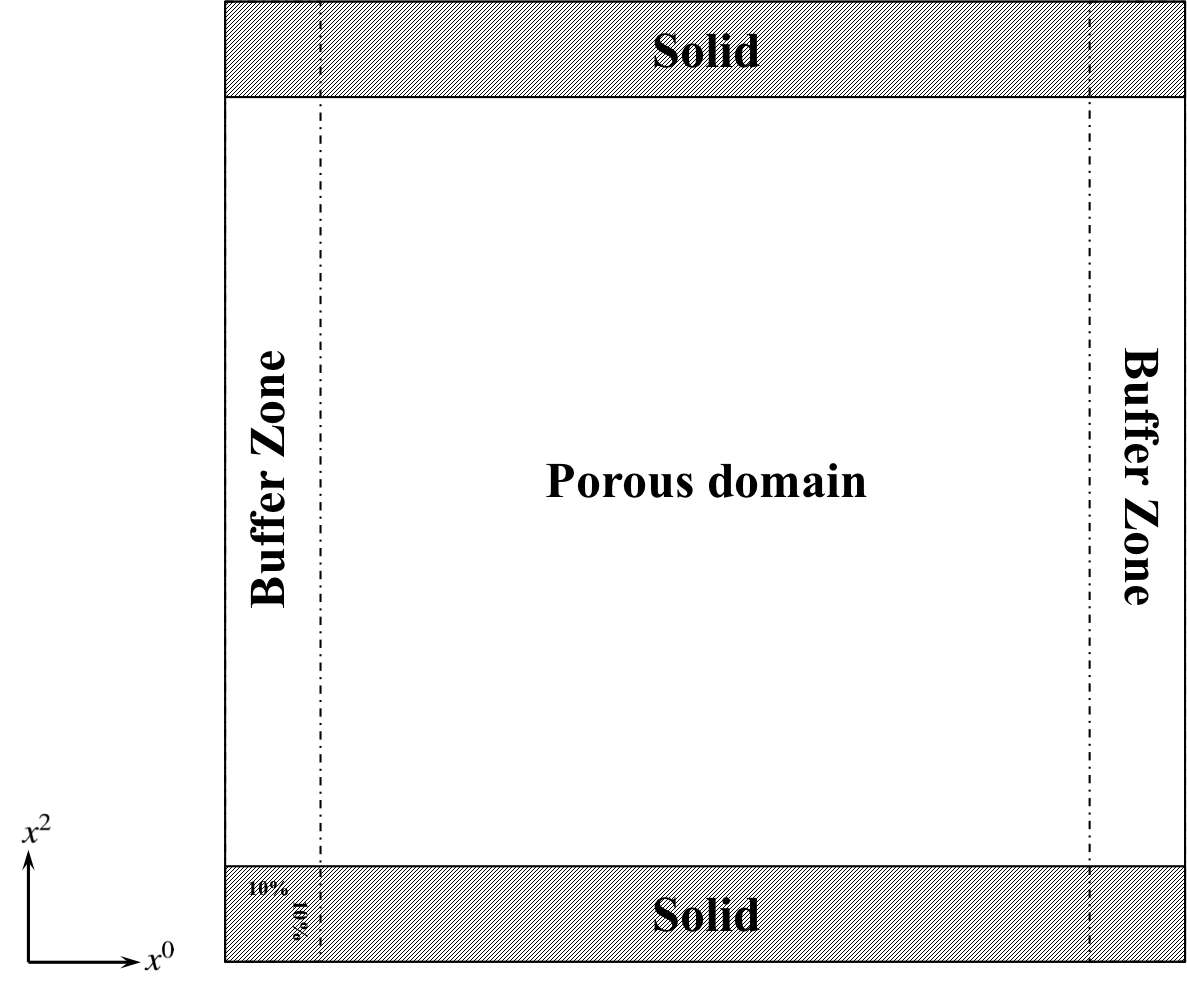
Refer to caption
Figure 7: A porous medium embedded in a square cross-section channel with buffer zones on both inlet and outlet (view in x1x^{1}-direction).

In this numerical experiment, we set the mesh resolution to h=1/124h=1/124. The buffers are 10%10\% on each side of the domain, i. e., the sample domain used for sphere pack is of size 100×100×100100\times 100\times 100 and faces SinS_{\mathrm{in}} and SoutS_{\mathrm{out}} are located 5%5\% inside the domain from the inflow and outflow boundaries. We choose the characteristic length xc=10−3​mx_{\mathrm{c}}=10^{-3}\,\mathrm{m}, the characteristic velocity vc=10−4​m​s−1v_{\mathrm{c}}=10^{-4}\,\mathrm{m}\,\mathrm{s}^{-1}, and the characteristic pressure pc=1​kg​m−1​s−2p_{\mathrm{c}}=1\,\mathrm{kg}\,\mathrm{m}^{-1}\,\mathrm{s}^{-2}, which yields Re=10−1\mathrm{Re}=10^{-1}, X=10−5X=10^{-5}. The magnitude of the velocity field and the pressure field at steady state are shown in Figure 8. The computation of the permeability of this sample in the direction parallel to the flow yields the following results:

permeability in x0-direction:\displaystyle\text{permeability in~}x_{0}\text{-direction:} k\displaystyle k~ =5505​mD,\displaystyle=~5505\,\mathrm{mD}~,
permeability in x1-direction:\displaystyle\text{permeability in~}x_{1}\text{-direction:} k\displaystyle k~ =4027​mD,\displaystyle=~4027\,\mathrm{mD}~,
permeability in x2-direction:\displaystyle\text{permeability in~}x_{2}\text{-direction:} k\displaystyle k~ =4763​mD.\displaystyle=~4763\,\mathrm{mD}~.
Refer to caption
Figure 8: Permeability estimation of sphere pack: magnitude of velocity field (top) and pressure field (bottom) at steady state. From left to right, the main flow directions are x0x_{0}-direction, x1x_{1}-direction, and x2x_{2}-direction, respectively.

4.6 Permeability estimation in Berea sandstone

Berea sandstone, also regarded as Berea Grit, as a type of sedimentary rock are widely distributed in nature. With suitable porosity and permeability, it has been recognized as one of the best samples in hydrogeology and it is frequently used as a source of laboratory material in petroleum industry for testing permeability. Depending on the sample, the order of permeability typically lies between 101​mD10^{1}\,\mathrm{mD} and 103​mD10^{3}\,\mathrm{mD} for a Berea sandstone core.

The porous medium used here has a resolution of 256×256×256256\times 256\times 256 voxels, which was created by micro-CT imaging of a Berea sandstone. The porosity of the rock sample is 0.20.2. As in the previous example with sphere-pack, we add buffer zones to the inlet and outlet faces and enclose the other boundary faces with solid rock. The computational domain is then embedded inside a squared pipe with mesh size h=1/320h=1/320 and each buffer zone occupying 10%10\% of the domain. The boundary conditions and the location of faces SinS_{\mathrm{in}} and SoutS_{\mathrm{out}} for computing average pressure and flux are the same as in Section 4.5.

We choose the characteristic length xc=10−3​mx_{\mathrm{c}}=10^{-3}\,\mathrm{m}, the characteristic velocity vc=10−4​m​s−1v_{\mathrm{c}}=10^{-4}\,\mathrm{m}\,\mathrm{s}^{-1}, and the characteristic pressure pc=1​kg​m−1​s−2p_{\mathrm{c}}=1\,\mathrm{kg}\,\mathrm{m}^{-1}\,\mathrm{s}^{-2}, which yields Re=10−1\mathrm{Re}=10^{-1} and X=10−5X=10^{-5}. At steady-state, the magnitude of the velocity field and the pressure field are shown in Figure 9. The numerical solutions yield the following results for the Berea sandstone sample:

permeability in x0-direction:\displaystyle\text{permeability in~}x_{0}\text{-direction:} k\displaystyle k~ =939.4​mD,\displaystyle=~939.4\,\mathrm{mD}~,
permeability in x1-direction:\displaystyle\text{permeability in~}x_{1}\text{-direction:} k\displaystyle k~ =1015.9​mD,\displaystyle=~1015.9\,\mathrm{mD}~,
permeability in x2-direction:\displaystyle\text{permeability in~}x_{2}\text{-direction:} k\displaystyle k~ =742.5​mD.\displaystyle=~742.5\,\mathrm{mD}~.
Refer to caption
Figure 9: Permeability estimation of Berea sandstone: magnitude of velocity field (top) and pressure field (bottom) at steady state. From left to right, the main flow directions are x0x_{0}-direction, x1x_{1}-direction, and x2x_{2}-direction, respectively.

5 Conclusion

In this paper, we propose a numerical method for solving the incompressible Navier–Stokes equations on micro-CT images of porous media. The method combines a pressure-correction algorithm with interior penalty discontinuous Galerkin. Results show the accuracy of the method for simple porous media with known analytical permeability values. Simulations on sphere-pack and Berea sandstone show the robustness of the method.

Acknowledgments

The authors thank Christopher Thiele (Rice University) and Prof. Walter Chapman (Rice University) for discussions. The authors acknowledge Shell International Exploration and Production Inc. for computational resources supporting.

Appendix A Diffusion Term

In model problem eq. 7, if the diffusion term −Δ​𝒗-\Delta{{\boldsymbol{v}}} is replaced by a generalized form −2∇⋅𝜺(𝒗)-2{\boldsymbol{\nabla}}\cdot{{\boldsymbol{\varepsilon}}{({\boldsymbol{v}})}}, then for open boundary problem the DG forms eqs. 8c and 8d should be modified as follows:

a𝜺​(𝒗,𝜽)=2​∑E∈ℰh∫E𝜺⁡(𝒗):𝜺⁡(𝜽)−2​∑e∈Γh∪∂ΩD∫e{|𝜺⁡(𝒗)⋅𝒏e|}⋅⟦𝜽⟧+2ϵ∑e∈Γh∪∂ΩD∫e{|𝜺(𝜽)⋅𝒏e|}⋅⟦𝒗⟧+σh∑e∈Γh​∂ΩD∫e⟦𝒗⟧⋅⟦𝒘⟧,\displaystyle\begin{split}a_{\boldsymbol{\varepsilon}}({\boldsymbol{v}},{\boldsymbol{\theta}})~=~&2\sum_{E\in\mathcal{E}_{h}}\int_{E}{\boldsymbol{\varepsilon}}({\boldsymbol{v}}):{\boldsymbol{\varepsilon}}({\boldsymbol{\theta}})-2\sum_{e\in\Gamma_{h}\cup\partial\Omega^{\mathrm{D}}}\int_{e}\{\hskip-1.79993pt|{{\boldsymbol{\varepsilon}}({\boldsymbol{v}})\cdot{\boldsymbol{n}}_{e}}|\hskip-1.79993pt\}\cdot\left\llbracket{{\boldsymbol{\theta}}}\right\rrbracket\\ &+2\epsilon\sum_{e\in\Gamma_{h}\cup\partial\Omega^{\mathrm{D}}}\int_{e}\{\hskip-1.79993pt|{{\boldsymbol{\varepsilon}}({\boldsymbol{\theta}})\cdot{\boldsymbol{n}}_{e}}|\hskip-1.79993pt\}\cdot\left\llbracket{{\boldsymbol{v}}}\right\rrbracket+\frac{\sigma}{h}\sum_{e\in\Gamma_{h}\partial\Omega^{\mathrm{D}}}\int_{e}\left\llbracket{{\boldsymbol{v}}}\right\rrbracket\cdot\left\llbracket{{\boldsymbol{w}}}\right\rrbracket~,\end{split}
b𝜺​(𝜽)=\displaystyle b_{\boldsymbol{\varepsilon}}({\boldsymbol{\theta}})~=~ 2​ϵ​∑e∈∂ΩD∫e(𝜺⁡(𝜽)⋅𝒏e)⋅𝒗D+σh​∑e∈∂ΩD∫e𝒗D⋅𝜽.\displaystyle 2\epsilon\sum_{e\in\partial\Omega^{\mathrm{D}}}\int_{e}\big({\boldsymbol{\varepsilon}}({\boldsymbol{\theta}})\cdot{\boldsymbol{n}}_{e}\big)\cdot{\boldsymbol{v}}_{\mathrm{D}}+\frac{\sigma}{h}\sum_{e\in\partial\Omega^{\mathrm{D}}}\int_{e}{\boldsymbol{v}}_{\mathrm{D}}\cdot{\boldsymbol{\theta}}~.

In addition, the pressure update postprocessing step eq. 11a should be changed to

pn\displaystyle p^{n}~ =pn−1+ϕn−XRe∇⋅𝒗n.\displaystyle=~p^{n-1}+\phi^{n}-\frac{\mathrm{X}}{\mathrm{Re}}\,{\boldsymbol{\nabla}}\cdot{{\boldsymbol{v}}^{n}}~.

The corresponding eq. 14a, in space discretization part, should also be changed to

(phn,χh)\displaystyle(p^{n}_{h},\chi_{h})~ =(phn−1,χh)+(ϕhn,χh)−XRe​(∇⋅𝒗hn,χh).\displaystyle=~(p^{n-1}_{h},\chi_{h})+(\phi^{n}_{h},\chi_{h})-\frac{\mathrm{X}}{\mathrm{Re}}\,({\boldsymbol{\nabla}}\cdot{{\boldsymbol{v}}^{n}_{h}},\chi_{h})~.

Note, the above equations comprise all of the changes that are necessary when modifying the numerical scheme.

References

References

  • [1] V. Girault, P.-A. Raviart, Finite element methods for Navier–Stokes equations: theory and algorithms, Vol. 5, Springer-Verlag, 1986.
  • [2] R. Temam, Navier–Stokes equations: theory and numerical analysis, Vol. 343, American Mathematical Soc., 2001.
  • [3] A. J. Chorin, Numerical solution of the Navier–Stokes equations, Mathematics of computation 22 (104) (1968) 745–762.
  • [4] J.-L. Guermond, P. Minev, J. Shen, An overview of projection methods for incompressible flows, Computer methods in applied mechanics and engineering 195 (44) (2006) 6011–6045.
  • [5] J. Blasco, R. Codina, Error estimates for an operator-splitting method for incompressible flows, Applied Numerical Mathematics 51 (1) (2004) 1–17.
  • [6] B. Rivière, Discontinuous Galerkin Methods for Solving Elliptic and Parabolic Equations: Theory and Implementation, Frontiers in Applied Mathematics, Society for Industrial and Applied Mathematics, 2008.
  • [7] J. S. Hesthaven, T. Warburton, Nodal discontinuous Galerkin methods: algorithms, analysis, and applications, Springer Science & Business Media, 2007.
  • [8] M. Piatkowski, S. Müthing, P. Bastian, A stable and high-order accurate discontinuous Galerkin based splitting method for the incompressible Navier–Stokes equations, Journal of Computational Physics 356 (2018) 220–239.
  • [9] B. Krank, N. Fehn, W. A. Wall, M. Kronbichler, A high-order semi-explicit discontinuous Galerkin solver for 3D incompressible flow with application to DNS and LES of turbulent channel flow, Journal of Computational Physics 348 (2017) 634–659.
  • [10] J. Dvorkin, N. Derzhi, E. Diaz, Q. Fang, Relevance of computational rock physics, Geophysics 76 (5) (2011) E141–E153.
  • [11] H. Andrä, N. Combaret, J. Dvorkin, E. Glatt, J. Han, M. Kabel, Y. Keehm, F. Krzikalla, M. Lee, C. Madonna, et al., Digital rock physics benchmarks—part II: Computing effective properties, Computers & Geosciences 50 (2013) 33–43.
  • [12] N. Saxena, R. Hofmann, F. O. Alpak, S. Berg, J. Dietderich, U. Agarwal, K. Tandon, S. Hunter, J. Freeman, O. B. Wilson, References and benchmarks for pore-scale flow simulated using micro-CT images of porous media and digital rocks, Advances in Water Resources 109 (2017) 211–235.
  • [13] C.-H. Bruneau, Boundary conditions on artificial frontiers for incompressible and compressible Navier–Stokes equations, ESAIM: Mathematical Modelling and Numerical Analysis 34 (2) (2000) 303–314.
  • [14] J. G. Heywood, R. Rannacher, S. Turek, Artificial boundaries and flux and pressure conditions for the incompressible Navier–Stokes equations, International Journal for Numerical Methods in Fluids 22 (1996) 325–352.
  • [15] R. Rannacher, Finite element methods for the incompressible Navier–Stokes equations, Fundamental directions in mathematical fluid mechanics (2000) 191–293.
  • [16] K. Shahbazi, An explicit expression for the penalty parameter of the interior penalty method, Journal of Computational Physics 205 (2) (2005) 401–407.
  • [17] Y. Epshteyn, B. Riviere, Estimation of penalty parameters for symmetric interior penalty Galerkin methods, Journal of Computational and Applied Mathematics 206 (2007) 843–872, doi:10.1016/j.cam.2006.08.029.
  • [18] V. Girault, B. Riviere, M. Wheeler, A discontinuous Galerkin method with nonoverlapping domain decomposition for the stokes and Navier–Stokes problems, Mathematics of Computation 74 (249) (2005) 53–84.
  • [19] P. Bochev, R. B. Lehoucq, On the finite element solution of the pure Neumann problem, SIAM review 47 (1) (2005) 50–66.
  • [20] M. Akbas, A. Linke, L. G. Rebholz, P. W. Schroeder, An analogue of grad-div stabilization in nonconforming methods for incompressible flows, arXiv preprint arXiv:1711.04442.
  • [21] F. Frank, C. Liu, F. O. Alpak, B. Rivière, A finite volume / discontinuous Galerkin method for the advective Cahn–Hilliard equation with degenerate mobility on porous domains stemming from micro-CT imaging, Computational Geosciences doi:10.1007/s10596-017-9709-1.
  • [22] C. R. Ethier, D. Steinman, Exact fully 3D Navier–Stokes solutions for benchmarking, International Journal for Numerical Methods in Fluids 19 (5) (1994) 369–375.
  • [23] J. Lekner, Viscous flow through pipes of various cross-sections, European Journal of Physics 28 (3) (2007) 521.