Optimal population transfer in combined Feshbach Resonance and STIRAP processPreprint: APS/123-QED
Abstract
We present a method for the creation and control of cold molecules that involves coherently combining Feshbach Resonances and STIRAP. We present analytical and numerical results showing how to optimize this process that can be implemented using techniques readily available in standard experimental setups. This will provide a link in the chain from atoms to ground state molecules and can serve as a building block towards more complex processes in coherent ultracold chemistry.
I Introduction
Ultracold molecules have many potential uses in prominent areas such as quantum computation Winkler et al. 2007, control of chemical reactions Danzl et al. 2008; Vitanov et al. 2001a; Vitanov et al. 2001b; Malinovsky, V. S. and Krause, J. L. 2001, fundamental measurements Kuznetsova et al. 2008, and few-body collision physics Danzl et al. 2008; Winkler et al. 2007. Their rich internal energy structure that makes them useful in these applications is the same property that makes creating these objects difficult. One standard method for creating these ultracold molecules involves first creating ultracold atoms, then using incoherent procedures such as magneto-association, also known as Feshbach Resonance (FR) Tiesinga et al. 1993; Courteille et al. 1998; Köhler et al. 2006; Julienne et al. 2004; Chin et al. 2010, to form vibrationally high energy molecules, and afterwards transfer the molecules into their ground state via STIRAP Vitanov et al. 2001a; Winkler et al. 2007; Shapiro et al. 2007; Bergmann et al. 1998. One of the side effects of this methodology is that the intermediate state, the vibrationally hot molecules, sit and wait for the incoherent process to end before being cooled using coherent techniques. This opens the door to lose population through environmental factors, such as collisions or decay to outside states. Taking inspiration from double STIRAP procedures Kuznetsova et al. 2008; Danzl et al. 2008 we look to coherently combine the process of magneto-association and STIRAP in an attempt to minimize the time these molecules remain in this unstable state. By chaining these two processes together in a coherent manner we create a toolkit for true deterministic and coherent ultracold chemistry. In this paper we describe how we approached this task and the numerical optimization that goes into creating an ideal case. The major shift in framework we made is viewing the process of magneto-association, otherwise known as a Feshbach Resonance (FR), through the lens of the well understood coherent process of Rapid Adiabatic Passage (RAP) Vitanov et al. 2001b; Malinovsky, V. S. and Krause, J. L. 2001; Grischkowsky and Loy 1975; Loy 1974; Grischkowsky 1976. With that shift, we attempt to find a suitable dark state for this process and optimize accordingly. Ideally this technique can be used to chain together other elementary processes in this Lego-type coherent fashion.
II Model Description
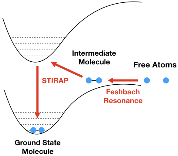
Our model describes a continuous, coherent process from ultraccold, separated atoms into ultracold molecules. Starting with separate atoms, we sweep through a Feshbach resonance to create a Feshbach molecule, i.e. a molecule in a highly excited vibrational state of the electronic ground state. Then we apply STIRAP to the resulting molecule to transfer the molecule into a lower energy state. The key factor that makes this method novel and useful compared to standard techniques is the coherent nature of the process. While common experimental techniques involve storing the Feshbach molecules in an optical trap and then performing STIRAP to cool them, our method is done in one continuous sweep to reduce the time the molecule spends in unstable intermediary states. Figure 1 shows a visualization of this process.

II.1 Model construction
Figure 2 is a visualization of the level scheme for this combined FR into STIRAP process. represents the state of separated ultracold atoms. represents the state of the newly combined Feshbach molecules. represents our end state of ground state molecules, and represents the intermediate molecular state of a standard STIRAP procedure. From this we get the following Hamiltonian for our four level system :
| (1) |
The ’s are detunings of levels from their bare atomic resonances. Our investigation will differ from other investigations into four-level systems Oreg et al. 1992; Band and Julienne 1991 in that we do not apriori assume certain detunings are identically zero or automatically enforce any n-photon resonances. In addition to the decay from out of the system, we have 3 other decay parameters. We have and from into and respectively, as well as from into . This model does not take into account any of the inefficiencies associated with standard FR processes, so population numbers reflect only the percentage of Feshbach molecules that are actually created via the initial magnetic field sweep, which typically is about 20% of the ultracold atom population. We also neglect to include decay from out of the system. From our numerical solutions the population spends negligible time in and thus extra decay from this level would have no effect.
II.2 Feshbach resonance as rapid adiabatic passage
To justify this model we treat FR as RAP. The Hamiltonian for a coupled two-channel model of FR is Köhler et al. 2006
The standard Hamiltonian for RAP is
According to Köhler et al. 2006 we can reduce the diagonal elements of to just the difference between the entrance and closed channels of the system, i.e. and . The optical detuning () of an RAP process is analogous to the magnetic detuning () in a FR process, while the Rabi frequencies () in RAP serve the same purpose as the level couplings () of FR in determining the width of the resonance. The similarity of both processes can be seen in their energy dynamics. This is shown in the appendix.
III Qualitative Analysis
Our goal is to maximize the coherent transfer of population from into . An easy way to do this would be to find a dark state of the Hamiltonian that has components of both and . Then we could adiabatically manipulate the parameters of our system such that the state initially is aligned along and ends fully aligned along . This is the bare minimum we are looking for at first. Once those conditions are satisfied we would like to impose further conditions of minimizing the amount of population that is in and throughout the process, as those states are assumed to be the most unstable and prone to decays out of the system. The first step in finding a dark state is looking at the determinant of the Hamiltonian
| (2) |
This is not identically zero, so no dark state exists apriori in this system. To move forward we artificially create one by enforcing certain relations between the parameters. First, note that this expression can be simplified by taking advantage of the freedom to set the zero energy of this system anywhere. Setting one of the detunings to 0 will negate some terms in this expression and make it more manageable. We choose to set , which reduces the complexity of the determinant to the last two terms in (2). These two terms cancel under following relation
| (3) |
With (3) the determinant of our Hamiltonian becomes 0 and the following unnormalized dark state appears
| (4) |
As desired this dark state has components along and . While there is an additional component along , there is no component along . Getting this dark state to initially line up with is difficult primarily because of the dark state condition (3). Our approximation is to start with and equal to , with and both nonzero. plays no significant role in this discussion, and is already by assumption. Our argument for this setup is that while technically all of the dark state components would be zero with these assignments, the components along and will be more strongly than the component along . The component along is a nonzero number multiplied by something very close to zero, whereas the components along and are the multiplication of two numbers very close to zero. At the end of our process we want the dark state to lie along , so in a similar fashion we choose and to be nonzero while and become or close to it. Other choices can be made for the detunings to set to 0, but they do little to simplify the problem. Setting results in a dark state with components along , , and while setting the other two detunings to zero results in a dark state with components along all four bare states. Throughout this procedure it will be useful to look at the coupling strengths between our dark state and other states in which we wish to avoid large populations. First we move into an adiabatic basis. We choose our dark state (4) and the excited state as two of the new basis vectors. then use Gram-Schmidt orthogonalization to get the remaining two basis states, which we will call bright states. The transformation matrix then becomes
where columns 1 and 2 are the bright states, column 3 is the excited state, and column 4 is our dark state. Sine the parameters in this matrix are time-dependent, this time-dependent transformation leads to the following transformed Hamiltonian
| (5) |
The coupling between the dark state and the excited state is identically 0 in this transformation. Therefore in our adiabatic considerations we focus on the coupling between the dark state and the two constructed bright states. By minimizing this coupling we should be able to stay in our dark state even in the presence of incoherent processes like decay in the system Wu et al. 2016
IV Numerical Results
In order to optimize the process and its timing, we employ numerical calculations. While the results shown here are not systematically optimized, combinations of intensity, detuning, time delays and processing speeds are shown here to demonstrate the power of the procedure compared to typical experimental setups.
A typical functional form of the Rabi frequencies that optimally maintain the coherence necessary for STIRAP consists of arctan-functions:
where , , and are the numerical parameters that form the search space. The form is such that for the ’s start (end) at 0 and end (start) at . We also take a similar form for , where starts near its maximal value and ends near . is numerically determined by the dark state condition (3).
Setting the decay rates and we found a typical evolution , represented by Fig. 3.

Figures (4) and (5) show the Rabi frequencies and detunings respectively needed to achieve this result. Note that the decay rates are near the magnitude of the Rabi frequencies needed to achieve this result. To help understand what these numbers mean, it’s useful to compare them with physically realizable parameters. Scaling the decay rate to the physically relevant quantity results in a maximal Rabi frequency of for Band and Julienne 1991.


This is a considerably better result than what can be achieved by treating the same four level system as two separate coherent processes of RAP followed by STIRAP, as seen in Fig. 6. This is a massive improvement for a medium-strength decay out of the system. While very strong decay out of the system will, up to now, produce similar results, this new method shows much improvement over treating these two processes independently.

Results for different combinations of system parameters (in particular, different strengths of decay out of state ) are shown in .
V Conclusion
This work provides a novel and easily testable framework for the creation of ultracold molecules. In addition, this coherent combination of the two steps can, in principle, be inserted anywhere needed in a chain of steps, joining together any resonant and STIRAP processes. Current experimental setups should be able to incorporate these ideas fairly easily, as the proposed method does not call for new equipment, merely an adjustment of standard techniques by adjusting to time dependent Rabi frequencies and detunings. One issue this work does not address yet is the relative inefficiency of the resonant process, particularly of Feshbach resonances. Due to the coherent nature of the STIRAP procedure, any combination of Feshbach resonance and STIRAP can only be used once, since repeated applications would empty the final state at the same rate as it would be filled. Further study into multiple iterations of this pulse scheme could mitigate that particular issue, altering this method to facilitate multiple runs that will capture more ground state molecules than are destroyed. This will be subject of an upcoming publication. Further improvement on the method presented here could be achieved by taking advantage of the strong coupling between the intermediate levels and Reiter and Sørensen 2012.
VI Acknowledgements
We would like to thank Robin Côtè and Florentin Reiter for helpful discussions. We would also like to acknowledge funding from the National Science Foundation.
Appendix A Explicit Hamiltonian
The entries from the transformed matrix mentioned in (5)
Appendix B Explicit parameter values
Appendix C Additional Graphs


Appendix D RAP and Feshbach Resonance energy structure

References
- Winkler et al. (2007) K. Winkler, F. Lang, G. Thalhammer, P. v. d. Straten, R. Grimm, and J. H. Denschlag, Phys. Rev. Lett. 98, 043201 (2007).
- Danzl et al. (2008) J. G. Danzl, E. Haller, M. Gustavsson, M. J. Mark, R. Hart, N. Bouloufa, O. Dulieu, H. Ritsch, and H.-C. Nägerl, Science 321, 1062 (2008), http://science.sciencemag.org/content/321/5892/1062.full.pdf .
- Vitanov et al. (2001a) N. Vitanov, M. Fleischhauer, B. Shore, and K. Bergmann, Advances In Atomic, Molecular, and Optical Physics, 46, 55 (2001a).
- Vitanov et al. (2001b) N. V. Vitanov, T. Halfmann, B. W. Shore, and K. Bergmann, Annual Review of Physical Chemistry 52, 763 (2001b), pMID: 11326080, https://doi.org/10.1146/annurev.physchem.52.1.763 .
- Malinovsky, V. S. and Krause, J. L. (2001) Malinovsky, V. S. and Krause, J. L., Eur. Phys. J. D 14, 147 (2001).
- Kuznetsova et al. (2008) E. Kuznetsova, P. Pellegrini, R. Côté, M. D. Lukin, and S. F. Yelin, Phys. Rev. A 78, 021402 (2008).
- Tiesinga et al. (1993) E. Tiesinga, B. J. Verhaar, and H. T. C. Stoof, Phys. Rev. A 47, 4114 (1993).
- Courteille et al. (1998) P. Courteille, R. S. Freeland, D. J. Heinzen, F. A. van Abeelen, and B. J. Verhaar, Phys. Rev. Lett. 81, 69 (1998).
- Köhler et al. (2006) T. Köhler, K. Góral, and P. S. Julienne, Rev. Mod. Phys. 78, 1311 (2006).
- Julienne et al. (2004) P. S. Julienne, E. Tiesinga, and T. Köhler, Journal of Modern Optics 51, 1787 (2004), https://www.tandfonline.com/doi/pdf/10.1080/09500340408232491 .
- Chin et al. (2010) C. Chin, R. Grimm, P. Julienne, and E. Tiesinga, Rev. Mod. Phys. 82, 1225 (2010).
- Shapiro et al. (2007) E. A. Shapiro, M. Shapiro, A. Pe’er, and J. Ye, Phys. Rev. A 75, 013405 (2007).
- Bergmann et al. (1998) K. Bergmann, H. Theuer, and B. W. Shore, Rev. Mod. Phys. 70, 1003 (1998).
- Grischkowsky and Loy (1975) D. Grischkowsky and M. M. T. Loy, Phys. Rev. A 12, 1117 (1975).
- Loy (1974) M. M. T. Loy, Phys. Rev. Lett. 32, 814 (1974).
- Grischkowsky (1976) D. Grischkowsky, Phys. Rev. A 14, 802 (1976).
- Cornish (2008) S. Cornish, Physics 1 (2008).
- Oreg et al. (1992) J. Oreg, K. Bergmann, B. W. Shore, and S. Rosenwaks, Phys. Rev. A 45, 4888 (1992).
- Band and Julienne (1991) Y. B. Band and P. S. Julienne, The Journal of Chemical Physics 95, 5681 (1991), https://doi.org/10.1063/1.461642 .
- Wu et al. (2016) Q.-C. Wu, Y.-H. Chen, B.-H. Huang, J. Song, Y. Xia, and S.-B. Zheng, Opt. Express 24, 22847 (2016).
- Reiter and Sørensen (2012) F. Reiter and A. S. Sørensen, Phys. Rev. A 85, 032111 (2012).