Fermionization of Bosons in a Flat Band

A quantum spin-liquid is one of the sought after states in a strongly interacting spin system. A recent neutron scattering experiment on herbertsmithite[1] reported the first detection of a spin-liquid phase. While the characterization of this state has been a matter of debate[2], this experiment indicates that the detection of the various spin-liquid states is not far away. Some manifestations of this state include a gapless Dirac (4-spinor) spin liquid state coupled to a U(1) gauge field[3, 4], a gapped $\mathrm{Z}_{2}$ spin liquid state[5, 2], a chiral spin liquid (CSL) [6, 7, 8, 9, 10, 11, 12, 13] some of which can also be gapless[14]. Such states exhibit absence of rotational symmetry breaking and, as such, do not stabilize any long-range magnetic order. Their collective low-energy excitations support fractionalized statistics, which can be classified using topological quantum field theory with various symmetry properties. Variety of techniques have been used in the literature to identify and study the properties of such states[15, 16, 17, 18] with many of the early and current attempts focusing on 2D triangular and honeycomb lattices[19, 20, 21, 22, 23].

Amongst the numerous quantum spin-liquid candidates[24, 25, 26, 27], the spin-$1/2$ Heisenberg magnet on a Kagome lattice stands out as a fascinating system that is believed to give rise to a variety of spin-liquid phases[28, 29]. The Kagome lattice is known to posses a flat band (quenched dispersion). If the lattice is sparsely populated by strongly interacting bosons (also referred to as hard-core bosons which avoid multiple occupancy of a single site), the state of the system is determined entirely from minimization of the interactions, since the kinetic energy of the system is fully quenched. Such a system is equivalent to an XY model with the $z$-directional magnetic field term, $H_{mag}=\sum_{\bf r}\mu S_{\bf r}^{z}$. The field strength $\mu$ maps on to the chemical potential of hard-core bosons. These bosons at low densities do not condense because of the degeneracy of the condensate wave functions which arises from the flat band. In the XY model, the absence of condensation translates to the absence of magnetic order. One is thus interested in learning about phases that can be stabilized in such a system.

It is instructive to note that if one replaces hard-core bosons by spinless fermions, the flat band would be capable accommodating fermionic states up to $\nu=1/3$, such that fermions avoid each other and have exactly zero energy (measured relative to the flat band) just by filling the flat band. This observation suggests that if there was a way for a system of hard-core bosons to stabilize low-energy excitations with fermionic statistics, such a state could be energetically favorable. In this article, we demonstrate the use of a technique that fermionizes hard-core bosons to find a chiral spin-liquid state as the energetically favorable candidate for the ground state of interacting spins on a Kagome lattice, which spontaneously breaks time-reversal symmetry (TRS) and represents an example where topological ordering is realized with interacting bosons.

Current understanding of the system under consideration is that the hard-core bosons can avoid paying any cost of interaction energy by forming spatially separated localized states[30, 31] which is possible due to the presence of a flat band in the Kagome lattice. Such a state can persist up to lattice filling of $\nu=1/9$, beyond which the system is faced with a choice between (a) populating higher energy bands (see Fig. 1); and (b) letting the bosons still reside in the flat band and paying the interaction cost due to overlap. The choice (a) would result in condensation of bosons (represented by (blue) dots on $E_{2}$ in Fig. 1) to the $\Gamma$ point of the Brillouin zone, leading to the supersolid state whose chemical potential grows as $\mu\sim(\nu-1/9)$, up to logarithmic prefactors. Such a supersolid state has been predicted as a mean-field theory for weakly interacting bosons at lattice fillings above $1/9$ in Ref. 31. The corresponding ground state energy $E_{GS}$ scales as $E_{GS}\sim(\nu-1/9)^{2}$.

The choice (b) essentially remains unexplored. We find within our approach that for strongly interacting bosons in a flat band Kagome lattice the correlations lead to effective fermionization of the bosons. To this end, we show that the system can still save energy (retaining $E_{\rm GS}\sim 0$) by continuing to populate the flat band up to $\nu=1/3$. Interestingly enough, the scaling of the chemical potential of the fermionized system with particle density is insensitive to the filling fraction around $1/9$, which is a critical value for condensed bosons. This change in the scaling of $\mu$ with density will result in different velocity distribution curves extracted from time-of-flight experiments on trapped atoms. This suggests that such an experiment can be used as a tool to distinguish between the two possible states, (a) and (b), under discussion, above the $1/9$ filling.

The fermionization of hard-core bosons relies on attaching a Chern-Simons(CS) phase, $\Lambda_{\{\mathbf{r}\}}$, to a fermionic many-body wavefunction: $|\Phi_{B}\rangle=e^{i\Lambda_{\{\mathbf{r}\}}}|\Psi_{F}\rangle$ (where $\{\mathbf{r}\}$ denotes the set of coordinates of the particles, $\Psi_{F}$ denotes the fermionic wavefunction, and $\Phi_{B}$ denotes the bosonic wavefunction). While this technique was used extensively to describe fractional quantum Hall(fQH) states[32, 33, 34, 35], it has also been applied to spin-orbit coupled bosons[36], bosons in honeycomb lattice[37], and bosons living on a moat[38]. It has been shown that fermionization can stabilize topological spin ordering[39, 40], high-temperature superconductivity[41], and even a chiral spin-liquid in a moat band[42]. In the latter case, the role of magnetic frustration is mapped to the degeneracy of the lowest single-particle states of the fermions (the moat-band). In this article, we device a scheme to fermionize bosons in a non-Bravais lattice in general which allows us to apply the fermionization technique to arbitrary lattices. For demonstration purposes, we apply our formulation to the case of Kagome lattice. We find that the trial wavefunction we propose, which by construction describes a CSL, is an eigenstate of the XY-model within a flux-smearing mean field approximation (MFA), and has the lowest many-body ground state energy. Our MFA breaks TRS and hence has non-zero flux per unit cell. The resulting spectrum has fermionic excitations and flux-flip excitations that can be understood as fractionally charged vortices with fractional self-statistics with angle $\theta=\frac{\pi}{2}$. These are semion excitations (which are examples of abelian anyons) of Kalmeyer-Laughlin CSL[15]. Moreover, the flat band prior to the MFA remains flat, but is now also gapped from the rest of the excited states. This provides a posteriori justification for the stability of our MFA. Indeed, using our trail wavefunction we explicitly demonstrate that the flux distribution within the unit cell is such that the flat band of the Kagome lattice is preserved upon the TRS breaking. This feature is unique to our prescription and unlike other attempts in literature to tackle a similar problem[6, 11, 12]. More explicitly, we set-up a trial wavefunction in the continuum limit (although this limit is not necessary) and demonstrate that our state has the lowest energy, potentially up to $\nu=1/3$.

It must be emphasized that the approach discussed in this article considers the effect of the CS field after the flux smearing MFA (which is consistent with the Gauss law constraint imposed by the CS terms in the original action). If one starts from the lattice gauge theory of CS field prior to the MFA[33, 11, 12, 43], it is not straightforward to converge to particular flux distribution, and the question of the TRS breaking remains an interesting open question. For this work, we wish to emphasize the usefulness of our variational MFA, in light of the previous results obtained in Refs. 36, 38, 42, 39, 41, which shows that the ground state can have the lowest possible energy from small occupation numbers all the way to the one-third filling of the lattice. Importantly, our result rules out the possibility of condensation of interacting bosons [choice (a) discussed above] in the vicinity of the $\nu=1/9$ filling fraction of the lattice. One can classify the possible CSLs based on symmetries, as done in some recent studies[44, 45]. The comprehensive classification of possible spin-liquid states based on the flux attachment procedure used in the present work is also possible, and is an open important problem that needs to be investigated in the future.

As indicated above, using fermionization technique, the CSL behavior has been suggested in systems with moats: which has a degenerate minima in the single particle spectrum. In this article we consider Kagome lattice which possess a flat band. We will discuss the differences arising in the calculation of many-body ground state energy in systems exhibiting moats and flat-bands. Finally we shall present the interesting avenues of research this approach motivates for future work.

The rest of the article is formatted as follows. Section II reviews the fermionization technique in general and presents a scheme to carry it out in a non-Bravais lattice (with multiple atoms per unit cell). In Sec. III we discuss the application of the scheme to Kagome lattice and show that the CSL trial wavefunction has the lowest ground state energy. Finally in Sec. IV we summarize the work and present an outlook for the fermionization technique. An appendix is included that presents technical details of some calculations which would have cluttered the presentation in the main text.

Let us start by summarizing the concept of fermionization. Consider a generic N-body Hamiltonian (on a Bravais lattice) $\hat{H}(\mathbf{r}_{1},...,\mathbf{r}_{N})\equiv\hat{H}(\{\mathbf{r}\})$. Let $|\Phi_{B}\rangle$ be the undetermined many-body bosonic wavefunction (subject to hard-shell constraint for the particles). The many-body ground state energy, $E_{\rm GS}$, for the hard-core bosons can be written as $E_{\rm GS}=\langle\Phi_{B}|\hat{H}(\{\mathbf{r}\})|\Phi_{B}\rangle$. The wavefunction $|\Phi_{B}\rangle$, describing hard core bosons can be expressed in a fermionic basis as $|\Phi_{B}\rangle=e^{i\Lambda_{\{\mathbf{r}\}}}|\Psi_{F}\rangle$, where $\Lambda_{\{\mathbf{r}\}}=\kappa\sum_{r^{\prime}<r}\theta_{\mathbf{r}\mathbf{r}^{\prime}}$ [$\theta_{\mathbf{r}\mathbf{r}^{\prime}}={\rm arg}(\mathbf{r}-\mathbf{r}^{\prime})$], $\kappa$ is an odd integer. Thus,

Here the non local vector potential $\mathbf{A}_{\{\mathbf{r}\}}\equiv\partial_{\mathbf{r}}\Lambda_{\{\mathbf{r}\}}$ enters into the Hamiltonian via covariant derivative $-i\partial_{\mathbf{r}}\rightarrow-i\partial_{\mathbf{r}}+\mathbf{A}_{\{\mathbf{r}\}}$. This amounts to a magnetic field of $\mathbf{B}(\mathbf{r})\equiv\mathbf{\nabla}\times\mathbf{A}_{\{\mathbf{r}\}}=\sum_{i}2\pi\kappa\delta(\mathbf{r}-\mathbf{r}_{i})$. While, the wavefunction $|\Psi_{F}\rangle$ in Eq. (1) is still undetermined, Eq (2) presents a way to estimate $E_{GS}$ and needs further explanation. To go from $\hat{H}(\{\mathbf{r}\},\mathbf{A}_{\{\mathbf{r}\}})$ to $\hat{H}^{MFA}(\mathbf{r},\mathbf{A}_{\mathbf{r}})$, we perform a flux-smearing MFA. The essence of this approximation is that $\mathbf{B}(\mathbf{r})=\sum_{i}2\pi\kappa\delta(\mathbf{r}-\mathbf{r}_{i})$ $\rightarrow 2\pi\kappa\langle\hat{n}(\mathbf{r})\rangle=2\pi\kappa\nu$. That is, the field that was pinned to every particle, is smeared and treated as uniform. This MFA is consistent with the Gauss law constraint ($B=2\pi\kappa\nu$) imposed by the CS field prior to performing the MFA.

An important distinction is to be made here. In the continuum limit, at large enough length scales such that $|\mathbf{r}|\sim l\gg 1/\sqrt{\rm density}$, the Gauss law constraint can be accounted for by introducing a local $\mathbf{A}_{\mathbf{r}}$ such that $\mathbf{\nabla}\times\mathbf{A}_{\mathbf{r}}=\mathbf{B}$. For the lattice version of this approximation, we require the constraint to be implemented at the level of ‘flux per unit cell’ (hence $B$ is related directly to $\nu$ in the above formulas and not the density). For the case of 1 atom per unit cell with nearest neighbor hoppings, the flux configuration of the CS field is no different from the usual Maxwell field. The wavefunctions $|\Psi_{c}\rangle$ in Eq. (2) is then formed from the slater determinant of the single particle states of $\hat{H}(\mathbf{r},\mathbf{A}_{\mathbf{r}})$.

For a non-Bravais lattice, neither the nature of flux smearing MFA, nor the construction of a variational many-body state is straightforward. When there are two (or more) atoms per unit cell, had we carried out the flux smearing approximation as for a Bravias lattice, there would be no distinction between the Maxwell-type field and CS field. We realize that small enough length scales $|\mathbf{r}|\sim$lattice constant, the flux distribution within a unit cell must depend on the relative locations of atoms within the unit cell. Thus it is possible to implement the Gauss-law constraint at the level of unit cell and still be left with a degree of freedom in distributing the flux internally in the unit cell. To implement this feature, we propose that this can be implemented by requiring that all the hops that form loops internal to the unit cell (not more that one sharing edge), must not enclose any flux. This is based on the observation that in the absence of CDW ordering, the homogeneous CS flux attachment preserves the fact that if there is a triangle composed of two nearest-neighboring and one next-nearest-neighboring sites, then there must be such triangle within the unit cell where two subsequent hops along the links of nearest-neighboring sites are equivalent to a single hop along the next-nearest-neighbor link, see approaches in Refs. 36, 38, 42, 39, 46.

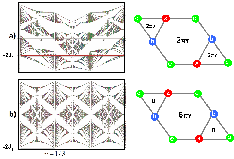
Note that if we have only one atom per unit cell (Bravais lattice), then there are no internal loops possible and thus the CS flux is the same as Maxwell flux. However, when we consider a non-Bravais lattice which contains loops of hops internal to the unit cell, there can be parts of the unit cell with zero net flux[38, 37]. This is seen by redrawing the unit cell as in Fig. 2b. The flux smearing field that confirms with the Gauss law can be accounted for by $\mathbf{A}_{\mathbf{r}}$ which introduces a flux $\phi_{T}$ per triangular region of the Kagome lattice. To account for the zero flux regions, one must introduce an intra-unit cell flux $\phi_{C}=\phi_{T}$ as in Figs. 2c,3. This introduction is lattice dependent and will be demonstrated later for the Kagome lattice.

Having demonstrated the non-triviality in the flux smearing MFA, we now address the subtlety in constructing the many-body wavefunction. The Hamiltonian matrix in a non-Bravais lattice has a rank, $n$, that is the number of atoms in the basis of the lattice. An $N$-body wavefunction can be denoted as $\Psi^{\{a\}}_{\{n\}}(\{\mathbf{r}\})\equiv\Psi_{n_{1},n_{2},...,n_{N}}^{a_{1},a_{2},...,a_{N}}(\mathbf{r}_{1},\mathbf{r}_{2},...,\mathbf{r}_{N})$, where a given coordinate $\mathbf{r}_{i}$ can describe the wavefunction component $a_{i}\in\{1,2,...,n\}$ in quantum state $n_{i}$. Correspondingly, the N-body Hamiltonian acquires the form $\hat{H}_{\{ab\}}(\{\mathbf{r}\})\equiv$

The presence of a basis in a non-Bravais lattice introduces a degree of freedom in implementing the antisymmetrization: if the single particle states are given by $\psi^{a}_{n}(\mathbf{r})$, where $n$ denotes the band and $a$ denotes the component of the wavefunction, the most general construction of a fermionic N-body state is

where $s,s_{i}\in\{1,2,...,N\}$, the repeated indices are summed over, and the Slater determinant is formed out of the indices $n_{i}$ and $\mathbf{r}_{i}$. The tensor $M$ superposes the anti-symmetrized Slater determinants for various combinations of $\{s_{i}\}$. The constraints on $M$ are enforced by requiring the many-body wavefunction be normalized to unity, and that the permutation properties of $M$ must respect antisymmetrization. This formally sets up a variational problem where the choice of the $M$-tensor is variational. The problem of such a huge variational space can be overcome by resorting to another technique to guess a trial wave-function, which we discuss next.

In general, the problem of hard core bosons on a lattice can be studied by looking at the spin-1/2 XY model with Hamiltonian

Here $S^{\pm}=S_{x}\pm iS_{y}$ are the spin-1/2 operators; the index $n$ scans all the neighbors at distance $m$; $\mathbf{r}_{m,n}$ is the vector to the $(m,n)^{\rm th}$ nearest neighbor. The choice of lattice is reflected in the choice various $\mathbf{r}_{mn}$. One choice of the phase attachment(in second-quantized notation) that accomplishes the CS transformation is[32, 33, 34]

where $c^{{\dagger}}_{\mathbf{r}}$ is a fermionic creation operator, and

This transforms the Hamiltonian to a fermionic basis:

where $\Lambda_{\mathbf{r}_{1},\mathbf{r}_{2}}\equiv\Lambda_{\mathbf{r}_{1}}-\Lambda_{\mathbf{r}_{2}}$ evaluated along the line joining $\mathbf{r}_{1}$ and $\mathbf{r}_{2}$. It is the analog of the accumulated phase $\int^{\mathbf{r}_{2}}_{\mathbf{r}_{1}}\mathbf{A}\cdot d\mathbf{l}$ in a lattice. Geometrically, $\Lambda_{\mathbf{r}_{1},\mathbf{r}_{2}}$ is the sum of the angles subtended by the vector $\mathbf{r}_{1}-\mathbf{r}_{2}$ at every other site (located at $\mathbf{r}^{\prime}$), weighted by the occupation probability of all sites along the path $\mathbf{r}_{1}\rightarrow\mathbf{r}_{2}$.

From here on we specialize to the Kagome lattice with the first neighbor hoppings. This is achieved by setting $m=1$, and letting $n$ scan from $1$ through $4$ (4 nearest neighbors) for each of the three atoms in the unit cell. The MFA leads to $c^{{\dagger}}_{\mathbf{r}}c_{\mathbf{r}}\rightarrow\langle c^{{\dagger}}_{\mathbf{r}}c_{\mathbf{r}}\rangle=n_{\mathbf{r}}=\nu$ (the filling fraction in the lattice) in the definition of $\Lambda_{\mathbf{r}}$. Let the lattice now be populated by hard-core bosons at every site with filling fraction $\nu$. Within our MFA, this provides non-zero flux at each site, spontaneously breaking TRS. The flux distribution is such that all the flux ($3\times 2\pi\nu\kappa$) is concentrated through the hexagon (Fig 3). To achieve this, one has to introduce two fluxes $\phi_{T}$ [to account for the Maxwellian field $\mathbf{A}_{\mathbf{r}}$], and $\phi_{C}$ (to account for the the intra unit cell flux modulation). In the absence of any external field, the CS field requires $\phi_{C}=\phi_{T}=3\pi\nu\kappa/4$.

We take note of the fact that the single particle ‘Hofstadter’ spectrum of this system is sensitive to the flux distribution within the unit cell. Figure 4a,b demonstrates that different flux distributions lead to different spectra. The property of the CS flux distribution seems to be that (i) the spectrum is unique up to $\nu=1/3$ at which point the flux through the unit cell is $2\pi$; (ii) the lowest energy band is still flat! We thus observe that a CS-flux distribution in the Kagome unit cell leads to an isolated flat band.

We now resort to calculating $E_{GS}$ where we will need the many-body trial wavefunction. To be explicit, we shall demonstrate this in the continuum limit. We iterate that to calculate $E_{GS}$ for the original Hamiltonian, we make an estimate using a trial wavefunction which is bosonic, but constructed out of a (fermionic) slater determinant by attaching a CS phase. The single particle states needed to construct this slater determinant are the eigenstates of the Hamiltonian obtained after the flux-smearing approximation. Further, since the original Hamiltonian has three bands, we focus of forming the slater determinant from the single particle states of the band in which the chemical potential is expected to lie. Since we will be addressing the low-density regime, we expect the chemical potential to lie in the lowest band. Using the projection technique introduced above, we can express $E_{GS}$ in terms of $E_{n}(\mathbf{r},\mathbf{r}^{\prime})$, where $n$ corresponds to the lowest flat band [see Eqs. (8)-(11)].

We choose $R^{a}_{n}$ and $\psi$ to be the eigenstates of the $\hat{H}^{\rm MFA}(\mathbf{r},\mathbf{A}_{\mathbf{r}})$. This estimate for $E_{GS}$ is expected to account for the non-local nature of $\mathbf{A}(\{\mathbf{r}\})$ and provide corrections to the many-body energy computed within MFA (Fig. 5). We shall explicitly demonstrate this in the continuum limit where the Hamiltonian in Eq. (12) after flux smearing can be written as:

where $H_{i}\equiv\left(e^{i\mathbf{p}\cdot\mathbf{a}_{i}/2}+e^{-i\mathbf{p}\cdot\mathbf{a}_{i}/2}\right),~i\in\{1,3\}$; $H_{2}\equiv\left(e^{i\mathbf{p}\cdot\mathbf{a}_{2}/2}+e^{-i\mathbf{p}\cdot\mathbf{a}_{2}/2}\right)e^{i\phi_{C}}$; $\mathbf{p}\equiv-i\partial_{\mathbf{r}}+\mathbf{A}_{\mathbf{r}}$, $p_{i}\equiv\mathbf{a}_{i}\cdot\mathbf{p}$; and $\mathbf{a}_{1}=a(1,0);~\mathbf{a}_{2}=a(1,\sqrt{3})/2;~\mathbf{a}_{3}=\mathbf{a}_{1}-\mathbf{a}_{2}$ are the translation vectors. It is understood that the Hamiltonian is to be expanded to $\mathcal{O}(p^{2})$. The resulting characteristic equation is

It can be shown that $E=0$ is a trivial solution. The eigenvalues are thus $E_{1}=-2J_{1}$, $E_{2/3}=J_{1}\left(1\mp\sqrt{9-3Ba^{2}(m+1/2)}\right)$, $m\in\{0,1,2,...\}$, and $\mathbf{B}=\mathbf{\nabla}\times\mathbf{A}_{\mathbf{r}}$. Note that the flat band $E_{1}$ is gapped from the rest of the dispersing bands($E_{2,3}$) by $3J_{1}(1-\sqrt{1-Ba^{2}/6})$. From Eq. (16), we note that the wavefunction components $\psi^{i}\equiv\int R^{i}\psi$ ($i\in{a,b,c}$) for $E_{1}$ satisfy

where $\phi_{T}\equiv\frac{\sqrt{3}}{16}Ba^{2}$ (measured counterclockwise). In the absence of any external magnetic field, the CS flux constraint requires $\phi_{T}=\phi_{C}$. Up to $\mathcal{O}(p^{2})$, we can also show that the wavefunction corresponding to $E_{1}$ and in quantum state $i$ is (see Appendix D) for calculation of $\mathcal{N}$):

where $\mathcal{N}$ is a normalization constant and $f_{i}(\mathbf{r})$ can be any function that decays stronger than $1/r^{2}$ (for normalizability). Similar to the Landau problem for free electrons, flat band wavefunctions in the presence of CS field are also inherently localized. To impose analyticity of the wavefunction, we postulate $f_{i}(\mathbf{r})=e^{-(\mathbf{r}-\mathbf{R}_{i})^{2}/2l^{2}_{CS}}$, where $\mathbf{R}_{i}$ is the center of the localized state, and $l_{CS}$ is an undermined localization length scale in the theory.

We prescribed a general scheme to construct the N-body wavefunction and compute the ground state energy of hard-core bosons in a non-Bravais lattice using fermionization. Using the example of the Kagome lattice, we showed that a CS type flux attachment can retain the massive degeneracy of system’s original electronic structure. Our trial wavefunction suggests that the ground state of hard-core bosons on a Kagome lattice is a spontaneously TRS broken chiral spin-liquid state. We proved that our trial wavefunction has zero statistical correction to the ground state energy due to a 2-dimensional degeneracy of the flat band in a Kagome lattice. It is thus a lowest energy state that implies absence of condensation of hard core bosons below third-filling (including the vicinity of the $\nu=1/9$ lattice filling fraction discussed above). While within our analysis, it is not possible to determine the uniqueness of this spin-liquid ground state, corroboration with other numerical techniques (e.g. DMRG) can help confirm this state.

The lattice itself can be realized using a cold atom set-up as in Ref. 49. In this reference, to ensure that the flat band is the lowest of the three, one can tune the lattice to the frustrated hopping regime with the help of artificial gauge fields attaching $\pi$ phases to all links resulting in the flipped sign of the matrix element. Other verifiable properties are bosonic edge states (can be detected using sudden decoupling technique[50]); and fractional excitations (time-of-flight experiments and Bragg spectroscopy[51, 52, 53]).

Acknowledgements: We are grateful to A. Kamenev and L. I. Glazman for useful discussions. T.A.S. thanks the Aspen Center for Physics (supported by National Science Foundation grant PHY-1607611) and the Max Planck Institute for the Physics of Complex Systems for hospitality. The work is supported by startup funds from UMass Amherst.

References

- [1] T.-H. Han, J. S. Helton, S. Chu, D. G. Nocera, J. A. Rodriguez-Rivera, C. Broholm, and Y. S. Lee, Nature 492, 406 EP (2012), URL http://dx.doi.org/10.1038/nature11659.
- [2] M. Punk, D. Chowdhury, and S. Sachdev, Nature Physics 10, 289 EP (2014), URL http://dx.doi.org/10.1038/nphys2887.
- [3] Y. Ran, M. Hermele, P. A. Lee, and X.-G. Wen, Phys. Rev. Lett. 98, 117205 (2007), URL https://link.aps.org/doi/10.1103/PhysRevLett.98.117205.
- [4] Y. Iqbal, F. Becca, and D. Poilblanc, Phys. Rev. B 84, 020407 (2011), URL https://link.aps.org/doi/10.1103/PhysRevB.84.020407.
- [5] S. Yan, D. A. Huse, and S. R. White, Science 332, 1173 (2011), ISSN 0036-8075, URL http://science.sciencemag.org/content/332/6034/1173.
- [6] K. Yang, L. K. Warman, and S. M. Girvin, Phys. Rev. Lett. 70, 2641 (1993), URL https://link.aps.org/doi/10.1103/PhysRevLett.70.2641.
- [7] L. Messio, B. Bernu, and C. Lhuillier, Phys. Rev. Lett. 108, 207204 (2012), URL https://link.aps.org/doi/10.1103/PhysRevLett.108.207204.
- [8] Y.-C. He, D. N. Sheng, and Y. Chen, Phys. Rev. Lett. 112, 137202 (2014), URL https://link.aps.org/doi/10.1103/PhysRevLett.112.137202.
- [9] S.-S. Gong, W. Zhu, and D. N. Sheng, Scientific Reports 4, 6317 EP (2014), article, URL http://dx.doi.org/10.1038/srep06317.
- [10] B. Bauer, L. Cincio, B. P. Keller, M. Dolfi, G. Vidal, S. Trebst, and A. W. W. Ludwig, Nature Communications 5, 5137 EP (2014), article, URL http://dx.doi.org/10.1038/ncomms6137.
- [11] K. Kumar, K. Sun, and E. Fradkin, Phys. Rev. B 90, 174409 (2014), URL https://link.aps.org/doi/10.1103/PhysRevB.90.174409.
- [12] K. Kumar, K. Sun, and E. Fradkin, Phys. Rev. B 92, 094433 (2015), URL https://link.aps.org/doi/10.1103/PhysRevB.92.094433.
- [13] M. P. Zaletel, Z. Zhu, Y.-M. Lu, A. Vishwanath, and S. R. White, Phys. Rev. Lett. 116, 197203 (2016), URL https://link.aps.org/doi/10.1103/PhysRevLett.116.197203.
- [14] R. G. Pereira and S. Bieri, SciPost Phys. 4, 004 (2018), URL https://scipost.org/10.21468/SciPostPhys.4.1.004.
- [15] V. Kalmeyer and R. B. Laughlin, Phys. Rev. Lett. 59, 2095 (1987), URL https://link.aps.org/doi/10.1103/PhysRevLett.59.2095.
- [16] X. G. Wen, F. Wilczek, and A. Zee, Phys. Rev. B 39, 11413 (1989), URL https://link.aps.org/doi/10.1103/PhysRevB.39.11413.
- [17] D. V. Khveshchenko and P. B. Wiegmann, Modern Physics Letters B 03, 1383 (1989), URL https://doi.org/10.1142/S0217984989002089.
- [18] D. V. Khveshchenko and P. B. Wiegmann, Modern Physics Letters B 04, 17 (1990), URL https://doi.org/10.1142/S0217984990000040.
- [19] A. Kitaev, Annals of Physics 321, 2 (2006), ISSN 0003-4916, january Special Issue, URL http://www.sciencedirect.com/science/article/pii/S0003491605002381.
- [20] H. Yao and S. A. Kivelson, Phys. Rev. Lett. 99, 247203 (2007), URL https://link.aps.org/doi/10.1103/PhysRevLett.99.247203.
- [21] C. Xu and S. Sachdev, Phys. Rev. B 79, 064405 (2009), URL https://link.aps.org/doi/10.1103/PhysRevB.79.064405.
- [22] A. Wietek and A. M. Läuchli, Phys. Rev. B 95, 035141 (2017), URL https://link.aps.org/doi/10.1103/PhysRevB.95.035141.
- [23] Y. Werman, S. Chatterjee, S. C. Morampudi, and E. Berg, Phys. Rev. X 8, 031064 (2018), URL https://link.aps.org/doi/10.1103/PhysRevX.8.031064.
- [24] L. Balents, Nature 464, 199 EP (2010), URL http://dx.doi.org/10.1038/nature08917.
- [25] L. Savary and L. Balents, Reports on Progress in Physics 80, 016502 (2017), URL http://stacks.iop.org/0034-4885/80/i=1/a=016502.
- [26] Y. Zhou, K. Kanoda, and T.-K. Ng, Rev. Mod. Phys. 89, 025003 (2017), URL https://link.aps.org/doi/10.1103/RevModPhys.89.025003.
- [27] O. Benton, L. D. C. Jaubert, R. R. P. Singh, J. Oitmaa, and N. Shannon, Phys. Rev. Lett. 121, 067201 (2018), URL https://link.aps.org/doi/10.1103/PhysRevLett.121.067201.
- [28] M. R. Norman, Rev. Mod. Phys. 88, 041002 (2016), URL https://link.aps.org/doi/10.1103/RevModPhys.88.041002.
- [29] R. Pohle, H. Yan, and N. Shannon, arXiv (2017), URL https://arxiv.org/abs/1711.03778.
- [30] D. L. Bergman, C. Wu, and L. Balents, Phys. Rev. B 78, 125104 (2008), URL https://link.aps.org/doi/10.1103/PhysRevB.78.125104.
- [31] S. D. Huber and E. Altman, Phys. Rev. B 82, 184502 (2010), URL https://link.aps.org/doi/10.1103/PhysRevB.82.184502.
- [32] J. K. Jain, Phys. Rev. Lett. 63, 199 (1989), URL https://link.aps.org/doi/10.1103/PhysRevLett.63.199.
- [33] A. Lopez and E. Fradkin, Phys. Rev. B 44, 5246 (1991), URL https://link.aps.org/doi/10.1103/PhysRevB.44.5246.
- [34] B. I. Halperin, P. A. Lee, and N. Read, Phys. Rev. B 47, 7312 (1993), URL https://link.aps.org/doi/10.1103/PhysRevB.47.7312.
- [35] S. C. Zhang, T. H. Hansson, and S. Kivelson, Phys. Rev. Lett. 62, 82 (1989), URL https://link.aps.org/doi/10.1103/PhysRevLett.62.82.
- [36] T. A. Sedrakyan, A. Kamenev, and L. I. Glazman, Phys. Rev. A 86, 063639 (2012), URL https://link.aps.org/doi/10.1103/PhysRevA.86.063639.
- [37] T. A. Sedrakyan, V. M. Galitski, and A. Kamenev, Phys. Rev. Lett. 115, 195301 (2015a), URL https://link.aps.org/doi/10.1103/PhysRevLett.115.195301.
- [38] T. A. Sedrakyan, L. I. Glazman, and A. Kamenev, Phys. Rev. B 89, 201112 (2014), URL https://link.aps.org/doi/10.1103/PhysRevB.89.201112.
- [39] T. A. Sedrakyan, V. M. Galitski, and A. Kamenev, Phys. Rev. B 95, 094511 (2017), URL https://link.aps.org/doi/10.1103/PhysRevB.95.094511.
- [40] R. Wang, B. Wang, and T. A. Sedrakyan, Phys. Rev. B 98, 064402 (2018), URL https://link.aps.org/doi/10.1103/PhysRevB.98.064402.
- [41] R. Wang, T. A. Sedrakyan, B. Wang, and D. Xing (2017), URL https://arxiv.org/abs/1712.06762.
- [42] T. A. Sedrakyan, L. I. Glazman, and A. Kamenev, Phys. Rev. Lett. 114, 037203 (2015b), URL https://link.aps.org/doi/10.1103/PhysRevLett.114.037203.
- [43] R. Sohal, L. H. Santos, and E. Fradkin, Phys. Rev. B 97, 125131 (2018), URL https://link.aps.org/doi/10.1103/PhysRevB.97.125131.
- [44] S. Bieri, L. Messio, B. Bernu, and C. Lhuillier, Phys. Rev. B 92, 060407 (2015), URL https://link.aps.org/doi/10.1103/PhysRevB.92.060407.
- [45] S. Bieri, C. Lhuillier, and L. Messio, Phys. Rev. B 93, 094437 (2016), URL https://link.aps.org/doi/10.1103/PhysRevB.93.094437.
- [46] S. Maiti and T. A. Sedrakyan, arXiv 1812.10153 (2019), URL https://arxiv.org/abs/1812.10153.
- [47] Y.-M. Lu and A. Vishwanath, Phys. Rev. B 86, 125119 (2012), URL https://link.aps.org/doi/10.1103/PhysRevB.86.125119.
- [48] X.-G. Wen, Advances in Physics 44, 405 (1995), eprint https://doi.org/10.1080/00018739500101566, URL https://doi.org/10.1080/00018739500101566.
- [49] G.-B. Jo, J. Guzman, C. K. Thomas, P. Hosur, A. Vishwanath, and D. M. Stamper-Kurn, Phys. Rev. Lett. 108, 045305 (2012), URL https://link.aps.org/doi/10.1103/PhysRevLett.108.045305.
- [50] M. Atala, M. Aidelsburger, M. Lohse, J. T. Barreiro, B. Paredes, and I. Bloch, Nature Physics 10, 588 EP (2014), article, URL http://dx.doi.org/10.1038/nphys2998.
- [51] J. Stenger, S. Inouye, A. P. Chikkatur, D. M. Stamper-Kurn, D. E. Pritchard, and W. Ketterle, Phys. Rev. Lett. 82, 4569 (1999), URL https://link.aps.org/doi/10.1103/PhysRevLett.82.4569.
- [52] A. M. Rey, P. B. Blakie, G. Pupillo, C. J. Williams, and C. W. Clark, Phys. Rev. A 72, 023407 (2005), URL https://link.aps.org/doi/10.1103/PhysRevA.72.023407.
- [53] P. T. Ernst, S. Götze, J. S. Krauser, K. Pyka, D.-S. Lühmann, D. Pfannkuche, and K. Sengstock, Nature Physics 6, 56 EP (2009), article, URL http://dx.doi.org/10.1038/nphys1476.