Bayesian inference in high-dimensional linear models using an empirical correlation-adaptive prior
Abstract
In the context of a high-dimensional linear regression model, we propose the use of an empirical correlation-adaptive prior that makes use of information in the observed predictor variable matrix to adaptively address high collinearity, determining if parameters associated with correlated predictors should be shrunk together or kept apart. Under suitable conditions, we prove that this empirical Bayes posterior concentrates around the true sparse parameter at the optimal rate asymptotically. A simplified version of a shotgun stochastic search algorithm is employed to implement the variable selection procedure, and we show, via simulation experiments across different settings and a real-data application, the favorable performance of the proposed method compared to existing methods.
Keywords and phrases: Collinearity; empirical Bayes; posterior convergence rate; stochastic search; variable selection.
1 Introduction
Consider the standard linear regression model
where is a vector of response variables, is a matrix of predictor variables, is a vector of regression coefficients, and is a vector of iid errors. We are interested in the high-dimensional case, where . Furthermore, it is assumed that the true is sparse, i.e., only a small subset of the coefficients are nonzero.
There are a variety of methods available for estimating under a sparsity constraint. This includes regularization-based methods like the lasso (Tibshirani, 1996), the adaptive lasso (Zou, 2006), the SCAD (Fan and Li, 2001), and MCP (Zhang, 2010); see Fan and Lv, 2010 for a review. From a Bayesian point of view, varieties of priors for regression coefficients and the model space have been developed, leading to promising selection properties. For the regression coefficients, , the normal mixture prior is specified in George and McCullogh, 1993; George and Foster, 2000 introduce empirical Bayes ideas; Ishwaran and Rao, 2005 use spike-and-slab priors; Bondell and Reich, 2012 estimate as the “most sparse” among those in a suitable posterior credible region; Polson and Scott, 2012 consider a horseshoe prior; Narisetty and He, 2014 use shrinking and diffusing priors; and Martin et al., 2017 consider an empirical Bayes version of spike-and-slab.
Collinearity is unavoidable in high-dimensional settings, and methods such as lasso tend to smooth away the regression coefficients of highly collinear predictors, and hence deter correlated covariates to be included in the model simultaneously. This motivated Krishna et al., 2009 to propose an adaptive powered correlation prior that lets the data itself weigh in on how collinear predictors are to be handled. However, their suggested generalized Zellner’s prior is not applicable in the scenario. To overcome this, we use an empirical Bayes approach, and propose an empirical correlation-adaptive prior (ECAP) to this framework. In Section 2, we present our empirical Bayes model and a motivating example illustrating the effect of correlation-adaptation in the prior. Asymptotic posterior concentration properties are derived in Section 3, in particular, adaptive minimax rates are established for estimation of the mean response. In Section 4, we recommend a shotgun stochastic search approach for computation of the posterior distribution over the model space. Simulation experiments are presented in Section 5, and we demonstrate the benefits of adaptively varying the correlation structure in the prior for variable selection compared to existing methods. The real-data illustration in Section 6 highlights the improved predictive performance that can be achieved using the proposed correlation-adaptive prior. Proofs of the theorems are deferred to the Appendix.
2 Model specification
2.1 The prior
Under assumed sparsity, it is natural to decompose as , where is the set of non-zero coefficients, called the configuration of , and is the -vector of non-zero values, with denoting the cardinality of . We will write for the sub-matrix of corresponding to the configuration . With this decomposition of , a hierarchical prior is convenient, i.e., a prior for and a conditional prior for , given .
First, for the prior for , we follow Martin et al., 2017 and write
where is a prior on and is a conditional prior on , given . Based on the recommendation in Castillo et al., 2015, we take
| (1) |
where and are positive constants, and . It is common to take to be uniform, but here we break from this trend to take collinearity into account. Let denote the determinant of , and consider the geometric mean of the eigenvalues, , as a measure of the “degree of collinearity” in model . We set
| (2) |
where is the condition number of , and and are positive constants specified to exclude models with extremely ill-conditioned . The constant is an important feature of the proposed model, and will be discussed in more detail below. Because of the dependence on above, we will henceforth write for the prior of .
Second, as the prior for , given , we take
| (3) |
Here is the least squares estimator corresponding to configuration and design matrix , is a shrinkage factor to be specified, is a parameter controlling the prior spread, is an adaptive powered correlation matrix, and
is a standardizing factor as in Krishna et al., 2009 designed to control for the scale corresponding to different values of . This data-driven prior centering is advantageous because we can use a conjugate normal prior, which has computational benefits, but without sacrificing on theoretical posterior convergence rate properties (Martin et al., 2017). Let denote this prior density for , given .
The power parameter on the prior covariance matrix can encourage or discourage the inclusion of correlated predictors. When , the prior shrinks the coefficients of correlated predictors towards each other; when , they tend to be kept apart, with being the most familiar; and, finally, implies prior independence. Therefore, positive would prefer larger models by capturing as many correlated predictors as possible, while negative tends to select models with less collinearity; see Krishna et al., 2009 for additional discussion of this phenomenon. Our data-driven choice of , along with that of the other tuning parameters introduced here and in the next subsection, will be discussed in Section 4.2.
2.2 The posterior distribution
For this standard linear regression model, the likelihood function is
It would be straightforward to include as an argument in this likelihood function, introduce a prior for , and carry out a full Bayesian analysis. However, our intention is to use a plug-in estimator for in what follows and, hence, we do not include the error variance as an argument in our likelihood function.
Given a prior and a likelihood, we can combine the two via Bayes’s formula to obtain a posterior distribution for or, equivalently, for the coefficient vector . To put a minor twist on this standard formulation, we follow a recent trend (Martin and Walker, 2014; Grünwald and van Ommen, 2017; Syring and Martin, 2017, e.g.,) and use a power likelihood instead of the likelihood itself. That is, our posterior for is defined as
where is the -vector obtained by filling in around with zeros in the entries corresponding to , and is a regularization factor. Then the posterior distribution for , denoted by , is obtained by summing over all configurations , i.e.,
Since one of our primary objectives is variable selection, it is of interest that we can obtain a closed-form expression for the posterior distribution of , up to a normalizing constant, a result of our use of a conjugate normal prior for , given . That is, we can integrate out above to get a marginal likelihood for , i.e.,
| (4) |
where is the eigenvalue of ; also, is the spectral decomposition of , with , and is the element of . Then it is straightforward to get the posterior distribution for :
| (5) |
The variable selection method described in Section 4 and illustrated in Sections 5–6 is based on this posterior distribution.
2.3 A motivating example
We now give a simple example to illustrate the effects of incorporating into (2) and (3). Consider a case with and let have iid rows, each with a standard multivariate normal with first-order autoregressive dependence and correlation parameter . Given , the conditional distribution of the response is determined by the linear model
The black, blue, and red curves in Figure 1 represent , for three different configurations, namely, the true configuration , , and , respectively. Panel (a) corresponds to a high correlation case, , we see that the ECAP-based posterior would prefer for suitably large ; compare this to the choice in Martin et al., 2017 which would prefer the smaller configuration . On the other hand, when the correlation is relatively low, as in Panel (b), we see that large positive would encourage larger configuration while the true configuration would be preferred for sufficiently large negative values of . The take-away message is that, by allowing to vary, the ECAP-based model has the ability to adjust to the correlation structure, which can be beneficial in identifying the relevant variables.


3 Posterior convergence properties
3.1 Setup and assumptions
We will stick with the standard notation given previously, but it will help to keep in mind that and are better understood as triangular arrays. Therefore, we can have , , and all depend on . We assume throughout that ; more precise conditions given below. We also assume that , , and are fixed constants in this setting, not parameters to be estimated/tuned. Therefore, to simplify the notation here and in the proofs, we will drop the subscript and simply write for the posterior for instead of .
For the fundamental problem of estimating the mean response, the minimax rate does not depend on the correlation structure in , so we cannot expect any improvements in the rate by incorporating this correlation structure in our prior distribution. Therefore, our goal here is simply to show that the minimax rates can still be achieved while leaving room to adjust for collinearity in finite-samples. The finite-sample benefits of the correlation-adaptive prior will be seen in the numerical results presented in Section 5.
We start by stating the basic assumptions for all the results that follow, beginning with two simple-to-state assumptions about the asymptotic regime. In particular, relative to , the true configuration is not too complex.
Assumption 1.
.
The next assumption puts a very mild size condition on the non-zero regression coefficients as well as on the user-specified shrinkage factor in the prior.
Assumption 2.
The true satisfies and, moreover, the factor satisfies .
The condition on above basically says that , which is typically much weaker than the usual beta-min condition—see (10) in Section 3.5—that is required for variable selection consistency. Note, however, that one would need to know to check this assumption about , and we present a data-driven choice of that satisfies this condition in Section 4.2.3.
Finally, we need to make some assumptions on the design matrix . For a given configuration , let and denote the smallest and the largest eigenvalues of , respectively. Next, define
Recall that these depend (implicitly) on because of the triangular array formulation. It is also clear that and are non-increasing and non-decreasing functions of the complexity , respectively. If is the condition number of , then we can define
and get the relation .
Assumption 3.
.
This assumption says, roughly, that every submatrix , for , is full rank, and is implied by, for example, the sparse Riesz condition of order in Zhang and Huang, 2008. More general results can surely be derived, i.e., with weaker conditions on , but at the expense of more complicated statements and assumptions.
3.2 Rates under prediction error loss
Define the set
| (6) |
which contains those that would do a relatively poor job of estimating the mean or, equivalently, of predicting the response . We, therefore, hope that the posterior assigns asymptotically negligible mass there. The following theorem makes this precise. Recall the definitions of the prior and, in particular, the quantities and .
Theorem 1.
Proof.
See Appendix A.2. ∎
In the so-called ordinary high-dimensional regime (Rigollet and Tsybakov, 2012, e.g.,), is the minimax concentration rate. So the take-away message here is, as long as the in (1) and (2) are chosen to satisfy
the ECAP posterior attains the minimax optimal rate.
3.3 Effective posterior dimension
Theorem 1 suggests that the posterior for concentrates near the true in some sense. However, since is sparse, it would be beneficial, for the sake of parsimony, etc, if the posterior also concentrated on a roughly -dimensional subset of . This does not follow immediately from the prediction loss result but, the following theorem reveals that the effective dimension of the posterior for is approximately .
Theorem 2.
Proof.
See Appendix A.3. ∎
Aside from the economical benefits of having an effectively low-dimensional posterior distribution, Theorem 2 is useful in the proofs of all the remaining results.
3.4 Rates under estimation error loss
Define the set
| (8) |
Just like in Section 3.2, we hope that, for suitable , the posterior will assign asymptotically negligible mass to this set of undesirable s.
Theorem 3.
Proof.
See Appendix A.4. ∎
Under Assumption 1 and 3, is bounded with probability . Hence, our rate is , better than the rate for lasso (Zhang et al., 2008).
3.5 Variable selection consistency
One of our primary objectives in introducing the -dependent prior distribution that accounts for collinearity structure in the design matrix is for the purpose of more effective variable selection. So it is imperative that we can demonstrate theoretically that, at least asymptotically, our posterior distribution will concentrate on the correct configuration . The following theorem establishes this variable selection consistency property.
Theorem 4.
Proof.
See Appendix A.5. ∎
The extra conditions on in Theorem 4 effectively require that the true configuration size, , is small relative to and, furthermore, that the constant in (1) is large enough that concentrates on comparatively small configurations. Also, the non-zero values are more difficult to detect if their magnitudes are small. This is intuitively clear, and also shows up in our simulation results for Cases 1–2 in Section 5. Theorem 4 gives a mathematical explanation of this intuition, stating that variable selection based on our empirical Bayes posterior will be correct asymptotically if the true signals have magnitude greater than the threshold in (10). This is the so-called beta-min condition; see, e.g., Bühlmann and van de Geer, 2011 or Arias-Castro and Lounici, 2014.
4 Implementation details
4.1 Stochastic search of the configuration space
In order to compute the posterior probability, we need to evaluate as defined in (2). The difficulty comes from the denominator of (2), i.e.,
where, again, is the determinant. Since and could be chosen large enough so that only extremely ill-conditioned cases would be excluded, there are approximately terms in the above summation. So brute-force computation can be done only for relatively small . Given that the eigenvalues are bounded from above and below for a given predictor matrix , is too, so it is not unreasonable to approximate the above summation by . This approximation is exact in the case of if all are included, and numerical experiments suggest that it is stable across a range of , , and . Therefore, using this approximation, the posterior distribution for that we use is given by
| (11) |
Markov chain Monte Carlo (MCMC) methods can be used to compute this posterior but this tends to be inefficient in high-dimensional problems. As an alternative, we employ the simplified shotgun stochastic search algorithm with screening (Shin et al., 2018, S5,), a simplified version of shotgun stochastic search (Hans et al., 2007, SSS,), to explore our posterior distribution. Different from traditional MCMC method, SSS does not attempt to approximate the posterior probability; instead, it only tries to explore high posterior probability regions as thoroughly as possible.
Here is a summary of our SSS algorithm. Let be a configuration of size , with , its corresponding (unnormalized) posterior. Define the neighborhood of as , where is the set containing all dimensional configurations that include , is the set containing all -dimensional configurations that only have one variable different from variables in , and is the set containing all -dimensional configurations that are nested in . The iteration of SSS goes as follows:
- 1.
Given , compute for all .
- 2.
Sample , , respectively from , , , with probabilities .
- 3.
Sample from with probabilities proportional to , , and , obtained by summing.
All visited configurations are recorded, and the final chosen configuration can be the maximum a posteriori model, median probability model (the model including those variables of which marginal inclusion probability is not less than ), or something else. For our simulations in Section 5, the selected configuration is the median probability model.
While SSS has the ability to explore many more high posterior configurations than MCMC, it is still computationally expensive, especially in high-dimensional case. For this reason, we adopt the S5 algorithm, which uses a screening technique to significantly decrease the computational cost.
4.2 Choice of tuning parameters
4.2.1 Choice of
An “ideal” value of is one that minimizes the Kullback–Leibler divergence of the marginal distribution from the true distribution of or, equivalently, one that maximizes the expected log marginal likelihood, i.e.,
Unfortunately, the ideal value is not available because we do not know the true distribution of , nor can we estimate it with an empirical distribution. However, a reasonable estimate of this ideal is
Indeed, Figure 2 shows for several different samples, along with an approximation of based on point-wise averaging. Notice that the individual log marginal likelihoods are maximized very close by where the expectation is maximized.

There is still one more obstacle in obtaining , namely, that we cannot directly compute the summation involved in due to the large number of configurations . Fortunately, we can employ an importance sampling strategy to overcome this. Specifically, we have
where are samples from . In our numerical results that follow, we use this to estimate defined above.
As discussed in Section 2.3, plays an important role in both model prior and coefficient prior. That is, for a fixed size , a positive favors model including predictors with relatively high correlation; a negative favors model including predictors with relatively low correlation; equals zero actually put equal mass on each model regardless of their predictors’ correlation structure. The in the conditional prior for , given , has a similar effect; see Krishna et al., 2009. Thus, a “good” estimate of should be such that it reflects the correlation structure in .
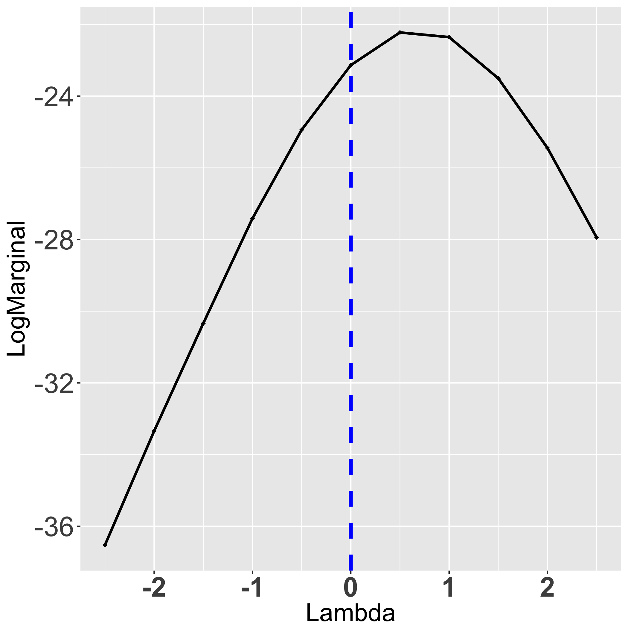
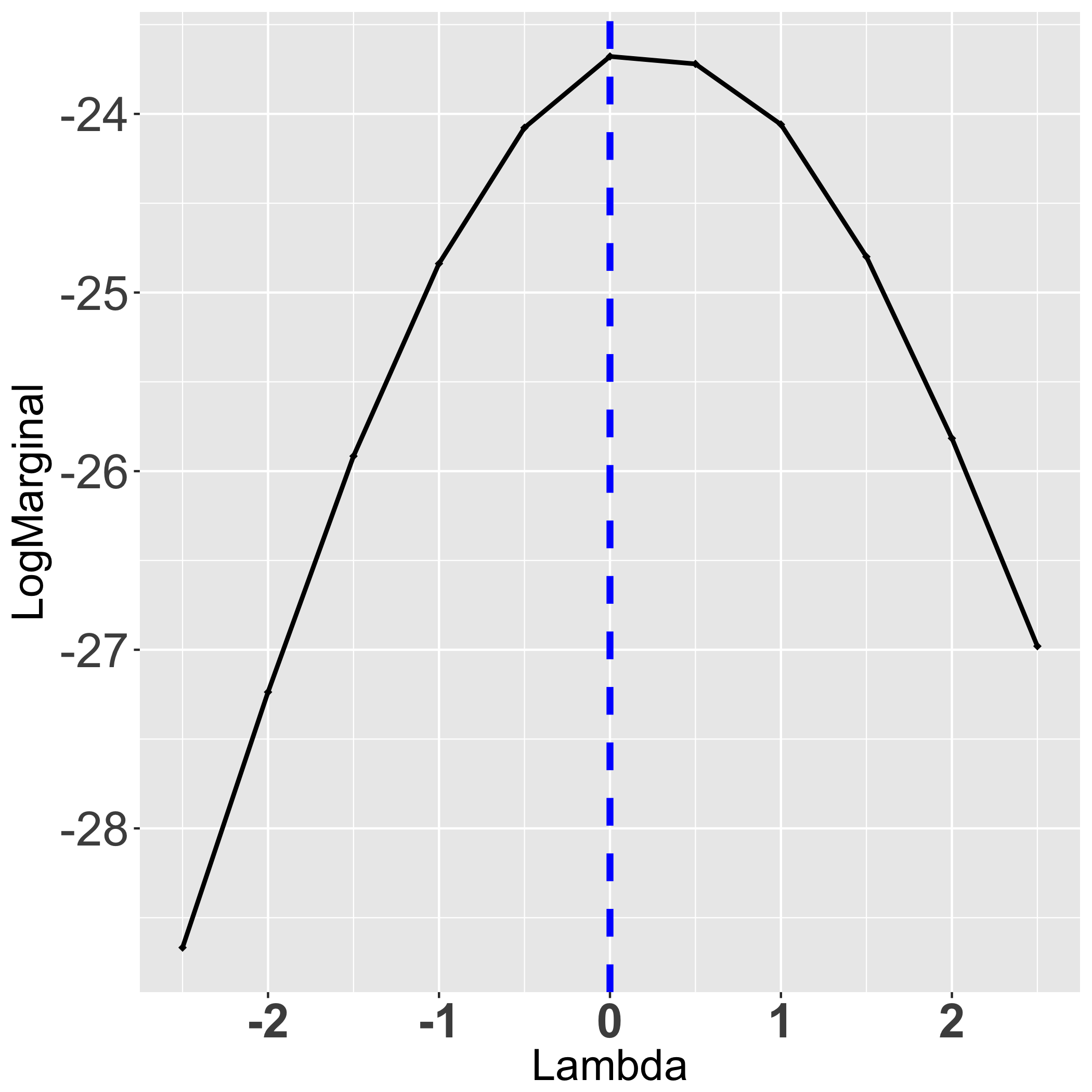
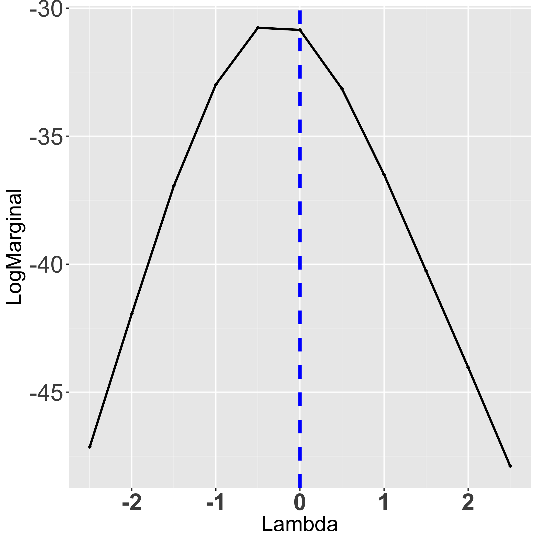
To help see this, consider a few examples, each with of dimension and , having an AR(1) correlation structure with varying correlation and true configuration . In particular, we consider two configurations:
Figure 3 shows chosen by maximizing the marginal likelihood in three different cases, and we argue that is at least in the “right direction.” In particular, when the true predictors are highly correlated, as in Panel (a), tends to be positive which encourages highly correlated predictors to be selected; and when the true predictors have low correlation, as in Panel (b), the estimate of is close to 0 hence a nearly uniform prior for . The situation in Panel (c) is different since the true predictors are minimally correlated while unimportant predictors are highly correlated. In this case, tends to be negative which discourages selecting the highly correlated ones that are likely unimportant.
4.2.2 Choice of
Now, recall that determines the magnitude of the prior variance of . If is sufficiently large, the conditional prior for is effectively flat; if is extremely tiny, then the posterior probability for will concentrate on the prior center . Kass and Wasserman, 1995 proposed the unit information criteria, which amounts to taking in the regression setting with Zellner’s prior. Foster and George, 1994 suggest a choice of . Here, we use a local empirical Bayes estimator for . That is, for given and , we choose a that maximizes the local marginal likelihood, that is,
In the special case where and , and a conjugate prior for , Feng et al., 2008 showed that , where is the usual statistic under model for testing . In general, our estimator, must be computed numerically.
4.2.3 Choice of
In our choice of , we seek to employ a meaningful amount of shrinkage while still maintaining the condition in Assumption 2. Towards this, if we view as a shrinkage estimator, then it is possible to choose so that the corresponding James–Stein type estimate has smaller mean square error. In particular, a that achieves this is
and, moreover, it can be shown that . Unfortunately, this still depends on , so we need to use some data-driven proxy for this. We recommend first estimating by from the adaptive lasso, with and the corresponding least squares estimators, and then setting
In practice, variable selection results are not sensitive to the choice of unless it is too close to 1. That is, according to Figure 4, we see good curvature in the log marginal likelihood for , with roughly the same maximizer, for a range of . The curves flatten out when is too close to 1, but that “too close” cutoff gets larger with , consistent with the assumption that . To ensure identifiability of , we manually keep our estimate of away from 1, in particular, we take .

4.2.4 Specification of remaining parameters
It remains to specify the likelihood power , the tuning parameters , specifying the prior on configuration size, and to specify a plug-in estimator for the error variance . As in Martin et al., 2017, we take , , and . For the error variance, we use the adaptive lasso to select a configuration and set equal to the mean square error for that selected configuration.
5 Simulation experiments
Here we investigate the variable selection performance of different methods in five simulated data settings. In each setting, and and the error variance is set to 1. The first two settings have severe collinearity. We employ the first order autoregressive structure with as the covariance structure of the design matrix ; and the true configuration includes two blocks of variables that the first block contains the 11th to the 15th variable and the second block contains the 31st to the 35th variable. We explored both large and small signal cases as follows.
- Case 1:
-
- Case 2:
-
- Case 3:
-
In this case, we consider a block covariance setting, which is the same as the Case 4 in Narisetty and He, 2014. In this setting, interesting variables have common correlation ; uninteresting variables have common correlation ; the common correlation between interesting and uninteresting ones is . The coefficients of the interesting variables are .
- Case 4:
-
This case is similar to Case 3, but let , , and . Also, a larger is adopted.
- Case 5:
-
This case is a low correlation case, which is set the same as Case 2 in Narisetty and He, 2014. All variables are set to have common correlation and the coefficients for interesting variables are .
For each case, 1000 data sets are generated. Denoting the chosen configuration as , we compute and in these 1000 iterations to measure the performance of our method, denoted by ECAP. For comparison purposes, we also consider the lasso (Tibshirani, 1996), the adaptive lasso (Zou, 2006), the smoothly clipped absolute deviation (Fan and Li, 2001, SCAD,), the elastic net (Zou and Hastie, 2005, EN,) and an empirical Bayes approach (Martin et al., 2017, EB,). Tuning parameters in the first four methods are chosen by BIC. The results are summarized in Table 1.
| Case | Method | Average | ||
|---|---|---|---|---|
| 1 | lasso | 0.082 | 0.996 | 13.61 (0.09) |
| alasso | 0.397 | 0.930 | 10.73 (0.04) | |
| EN | 0.133 | 0.983 | 13.24 (0.20) | |
| SCAD | 0 | 0.001 | 12.36 (0.15) | |
| EB | 0.165 | 0.215 | 9.56 (0.17) | |
| ECAP | 0.263 | 0.342 | 9.65 (0.15) | |
| 2 | lasso | 0.297 | 1 | 11.65 (0.05) |
| alasso | 0.356 | 0.412 | 9.33 (0.03) | |
| EN | 0.557 | 0.816 | 10.25 (0.07) | |
| SCAD | 0 | 0 | 7.93 (0.04) | |
| EB | 0.815 | 1 | 11.27 (0.91) | |
| ECAP | 0.994 | 1 | 10.00 (0.00) | |
| 3 | lasso | 0 | 0.874 | 18.67 (0.12) |
| alasso | 0.002 | 0.277 | 11.26 (0.10) | |
| EN | 0 | 0.945 | 19.82 (0.22) | |
| SCAD | 0.882 | 0.958 | 5.05 (0.01) | |
| EB | 0.560 | 0.670 | 4.69 (0.05) | |
| ECAP | 0.760 | 0.778 | 4.90 (0.08) | |
| 4 | lasso | 0.135 | 1 | 8.08 (0.09) |
| alasso | 0.701 | 0.940 | 5.34 (0.03) | |
| EN | 0.327 | 0.997 | 7.33 (0.13) | |
| SCAD | 0.070 | 0.148 | 4.45 (0.04) | |
| EB | 0.793 | 0.822 | 4.87 (0.04) | |
| ECAP | 0.861 | 0.940 | 5.05 (0.07) | |
| 5 | lasso | 0.001 | 0.990 | 17.55 (0.15) |
| alasso | 0.057 | 0.693 | 8.63 (0.11) | |
| EN | 0.005 | 0.991 | 17.04 (0.28) | |
| SCAD | 0.419 | 0.908 | 5.88 (0.04) | |
| EB | 0.680 | 0.795 | 4.82 (0.04) | |
| ECAP | 0.827 | 0.919 | 4.95 (0.05) |
According to these results, ECAP performs significantly better than lasso, SCAD, and EN in terms of the probability of choosing the true configuration. It also has uniformly better performance compared with EB, which is expected since the new ECAP method takes the correlation information into account. However, when considering , ECAP is not always the highest, e.g., Case 1. Note that and for ECAP are always close to each other, which is not the case for lasso or EN. This is because the ECAP method is more likely to shrink the coefficients of unimportant predictors to zero, which is desirable if the goal is to find the true .
6 Real-data illustration
In this section, we examine our method in a real data example and evaluate its performance against other prevalent approaches including lasso, SCAD and the penalized credible region approach in Bondell and Reich, 2012. We use the data from an experiment conducted by Lan et al., 2006 that studies the genetics of two inbred mouse populations (B6 and BTBR). The data include gene expressions of 31 female and 29 male mice. Some phenotypes, including phosphoenopiruvate (PEPCK) and glycerol-3-phosphate acyltransferase (GPAT) were also measured by quatitative real-time PCR. The data are available at Gene Expression Omnibus data repository (http://www.ncbi.nlm.nih.gov/geo; accession number GSE3330).
We choose PEPCK and GPAT as response variables. Given that this is an ultra-high dimensional problem, we use marginal correlation based screening method, to screen down from genes to genes. Combining the screened 1999 genes with the sex variable, the final dimension of the predictor matrix is . After screening, we apply our method to the data and select a best subset of predictors . Then we use the posterior mean of as the estimator for , for given and . The posterior distribution for is normal with
where . For hyperparameters , and , we can plug in their corresponding estimators which can be obtained in the same way as in Section 4.
In order to evaluate the performance of our approach, we randomly split the sample into a training data set of size 55 and a test set of 5. First, we apply our variable selection method to the training set and obtain the selected variables. Then conditioning on this model, we estimate the regression coefficients using the above method. Based on the estimated regression coefficient, we predict the remaining 5 observations and calculate the prediction loss. This process is repeated 100 times, and an estimated mean square prediction error (MSPE) along with its standard error can be computed; see Table 2.
| PEPCK | GPAT | |||
|---|---|---|---|---|
| Method | MSPE | Model Size | MSPE | Model Size |
| ECAP () | 1.02 (0.07) | 5.04 (0.19) | 2.26 (0.18) | 8.34 (0.33) |
| lasso () | 3.03 (0.19) | 7.70 (0.96) | 5.03 (0.42) | 3.30 (0.79) |
| BCR.joint () | 2.03 (0.14) | 9.60 (0.46) | 3.83 (0.34) | 4.20 (0.43) |
| BCR.marginal () | 1.84 (0.14) | 23.3 (0.67) | 5.33 (0.41) | 21.8 (0.72) |
| SIS+SCAD () | 2.82 (0.18) | 2.30 (0.09) | 5.88 (0.44) | 2.60 (0.10) |
| ECAP () | 0.72 (0.07) | 4.93 (0.30) | 1.66 (0.52) | 7.92 (0.73) |
In Table 2, BCR.joint and BCR.marginal denote methods using joint credible sets and marginal credible sets respectively, for details, see Bondell and Reich, 2012. The first four methods, ECAP, lasso, BCR.joint and BCR.marginal are implemented on the screened data with dimension . The fifth row is the results of sure independence screening (SIS) combined with SCAD applied to the full data and the last row is the outcomes from directly applying ECAP to unscreened dataset. The stopping rules of lasso, SCAD, BCR.joint and BCR.marginal are based on BIC.
In terms of MSPE, ECAP outperforms all the other methods significantly in both PEPCK and GPAT cases, given the estimated standard errors. Moreover, the MSPE from ECAP is even smaller for the full dataset compared with the screened data. And for the model size, on average, ECAP, lasso, BCR.joint and SIS+SCAD select models with comparable sizes while BCR.marginal always chooses larger models. Overall, ECAP performs very well in this real data example compared to these other methods in terms of both MSPE and model size.
Acknowledgments
The work presented herein is partially supported by the U.S. National Science Foundation, grant DMS–1737933.
Appendix A Technical details
A.1 Preliminary lemmas
Before getting to the proofs of the main theorems, we need to suitably lower-bound the posterior denominator and upper-bound the posterior numerator, the latter depending on the type of neighborhood being considered. In particular, for a generic measurable subset of the parameter space, write
where is the likelihood ratio, with the -vector corresponding to with zeros filled in around the indices in . Lemma 1 gives a general lower bound on the denominator .
In what follows, will denote the true and sparse coefficient vector in , with the corresponding configuration of complexity .
Lemma 1.
Given , define
where is the condition number of . Then under Assumptions 1–4, the denominator satisfies as .
Proof.
Since is a sum of non-negative terms, we get the trivial bound
where
are both non-negative, and the matrix is defined as
| (12) |
From the well-known sampling distribution of , we have
Next, for , under Assumption 3, it can be verified that the maximal eigenvalue of is . Therefore, . Since
and the first term is , it follows from Assumptions 1 and 2 that . This implies that which, in turn, implies that the exponential term in the lower bound for is no smaller than 1. Therefore,
and the product can be lower-bounded by for as defined above. Finally, we have that with vanishing -probability, as was to be shown. ∎
Next is an upper bound on the posterior numerator, , where is the complement of a neighborhood like that in (6), relevant to Theorem 1.
Lemma 2.
There exists a constant such that
where
where and depends only on .
Proof.
Let us consider the expectation of , given the true distribution of y, i.e. . Then by Hölder’s inequality, for constants and , we can find an upper bound for ,
| (13) |
where
If , then the Renyi divergence formula gives that
| (14) |
where the -dimensional vector is an augmented form of with if . Next, for , after factoring out the non-stochastic terms in the multivariate normal density, there is an expectation of exponential quadratic form to be dealt with, i.e.,
| (15) |
where and is the least square estimator under configuration . Let denote the mean of , then . Applying a spectral decomposition on in , we have,
where . is a diagonal matrix whose diagonal elements are the corresponding eigenvalues, and is a matrix with columns being corresponding eigenvectors. It is not difficult to show,
which implies are iid , where is the eigenvalue of and is the eigenvector. Hence, has a non-central distribution with non-centrality parameter . By taking advantage of the independence of s and using the moment generating function of the non-central chi-square distribution, (15) can be written as,
| (16) |
where . It is clear that (16) is a non-decreasing function with respect to . And when , . Then , we can obtain an upper bound for (15) by replacing with in (16),
| (17) |
For and , we can get the same expression of with and respectively. Therefore,
| (18) |
Since and are non-negative, we upper-bound the integral in (13) by
| (19) |
By plugging (18) and (14) into (19), and integrating out , we bound by,
where function is defined as above. ∎
A.2 Proof of Theorem 1
With Lemmas 1 and 2, the expectation of posterior probability of event , which is defined in (6), can be bounded by,
While for the prior, if , we can get,
Therefore the upper bound for the posterior probability can be written as,
where
Taking logarithm on both sides, we get
| (20) |
We require to have a certain rate such that the upper bound for posterior probability can vanish. A preliminary requirement for is , in order make as . In addition, should satisfy . Therefore, as , and . Thus, for any satisfying , we will have
Next, we establish the rate for . Under Assumption 1 and 2, is bounded with probability 1. By Stirling’s formula, we have that
Given that , we can also have
Since we have ruled out cases with extremely ill-conditioned , is bounded above by . Thus, for the nonnegative case,
Therefore, when , the rate of should be
The proofs for are similar. Therefore, the rate then can be rewritten as
where function has already been defined in Theorem 1.
A.3 Proof of Theorem 2
Followed by Lemma 2 and Theorem 1, we can get
Then it is not difficult to show that,
With the help of Lemma 1, the posterior probability of event can be bounded as,
| (21) |
From Theorem 1, we have
In addition, for , if , we can get
When , , then dominates the other two terms in (21). Therefore, will vanish as . Similarly for , we can get the same result if .
A.4 Proof of Theorem 3
A.5 Proof of Theorem 4
We segment the proof11 1 Some of the arguments presented here refer to Martin et al., 2017, but there are some oversights in the selection consistency results presented in the published version of that paper. The version available at arXiv:1406.7718 contains corrections of those arguments. of Theorem 4 into two parts. First, under Assumptions 1 and 3, we aim to show that, . Second, under the beta-min condition, we prove that . We only consider positive case here. The proofs in Parts 1 and 2 below can go through the same way when .
Part 1
Let be any configuration containing but not equal to the true model , i.e. . Then the posterior for can be written as,
where , is as in (12), and
Applying Hölder’s inequality with the same constants in (13), and , we get that is upper-bounded by
| (22) |
First, given that , is idempotent and . Therefore, has a central chi-square distribution . If , using moment generating function of central chi-square, the first expectation term in (22) can be written as,
Second, from the spectral decomposition , if , then,
Obviously, , and this implies . It follows that the s are independent non-central chi-square random variables, with non-centrality parameter and degrees of freedom of . Using the same argument as in (16)–(17), we get,
where . Since , we have
Also, by Assumptions 2 and 3, the exponential term is asymptotically bounded by . Therefore, we can conclude that the second expectation term in (22) is also asymptotically upper-bounded by .
Next, it is clear that
Since satisfies
and the lower and upper bounds are stable according to Assumption 3, it follows that is upper-bounded by , where .
For , as in Appendix A.2, we have
Now we can bound above by,
where and is a constant. By Theorem 2, we only need to consider configurations of size no more than , where in (7) and . Therefore,
| (23) |
Under Assumption 3, is bounded, so following the results in Martin et al., 2017, (23) turns out to be,
So, if and are such that , then will go to as .
Part 2
Consider a configuration satisfying , in Part 1, we already have (22), which is
For the first expectation term, if we plug in , where , then according to the results in Martin et al., 2017
Since and are independent, using the moment generating function of normal and chi-square distributions, we can get,
| (24) |
With some algebraic manipulation, we can show that
and then based on Lemma 5 of Arias-Castro and Lounici, 2014, we get
By the beta-min condition (10), it follows that , and, hence,
Then following the results in Martin et al., 2017, we can get,
When , we have,
When , we have,
Furthermore, if satisfies , the two fractions above will finally go to as and go to infinity.
References
- Arias-Castro and Lounici, (2014) Arias-Castro, E. and Lounici, K. (2014). Estimation and variable selection with exponential weights. Electron. J. Statist., 8(1):328–354.
- Bondell and Reich, (2012) Bondell, H. D. and Reich, B. J. (2012). Consistent high-dimensional Bayesian variable selection via penalized credible regions. J. Amer. Statist. Assoc., 107:1610–1624.
- Bühlmann and van de Geer, (2011) Bühlmann, P. and van de Geer, S. (2011). Statistics for High-Dimensional Data: Methods, Theory and Applications. Springer Science & Business Media.
- Castillo et al., (2015) Castillo, I., Schmidt-Hieber, J., and van der Vaart, A. (2015). Bayesian linear regression with sparse priors. Ann. Statist., 43:1986–2018.
- Fan and Li, (2001) Fan, J. and Li, R. (2001). Variable selection via nonconcave penalized likelihood and its oracle properties. J. Amer. Statist. Assoc., 96:1348–1360.
- Fan and Lv, (2010) Fan, J. and Lv, J. (2010). A selective overview of variable selection in high dimensional feature space. Statist. Sinica, 20:101–148.
- Feng et al., (2008) Feng, L., Rui, P., German, M., Merlise, A., and Jim, O. (2008). Mixtures of g priors for Bayesian variable selection. J. Amer. Statist. Assoc., 103:410–423.
- Foster and George, (1994) Foster, D. P. and George, E. I. (1994). The risk inflation criterion for multiple regression. Ann. Statist., 22:1947–1975.
- George and Foster, (2000) George, E. I. and Foster, D. P. (2000). Calibration and empirical Bayes variable selection. Biometrika, 87:731–747.
- George and McCullogh, (1993) George, E. I. and McCullogh, R. E. (1993). Variable selection via Gibbs sampling. J. Amer. Statist. Assoc., 88:881–889.
- Grünwald and van Ommen, (2017) Grünwald, P. and van Ommen, T. (2017). Inconsistency of Bayesian inference for misspecified linear models, and a proposal for repairing it. Bayesian Anal., 12(4):1069–1103.
- Hans et al., (2007) Hans, C., Dobra, A., and West, M. (2007). Shotgun stochastic search for large regression. J. Amer. Statist. Assoc., 102:507–517.
- Ishwaran and Rao, (2005) Ishwaran, H. and Rao, J. S. (2005). Spike and slab gene selection for multigroup microarray data. J. Amer. Statist. Assoc., 100:764–780.
- Kass and Wasserman, (1995) Kass, R. E. and Wasserman, L. (1995). A reference Bayesian test for nested hypotheses and its relationship to the schwarz criterion. J. Amer. Statist. Assoc., 90:928–934.
- Krishna et al., (2009) Krishna, A., Bondell, H., and Ghosh, S. K. (2009). Bayesian variable selection using an adaptive powered correlation prior. J. Statist. Plann. Inference, 139:2665–2674.
- Lan et al., (2006) Lan, H., Chen, M., Flowers, J. B., Yandell, B. S., Stapleton, D. S., Mata, C. M., Mui, E. T.-K., Flowers, M. T., Schueler, K. L., Manly, K. F., et al. (2006). Combined expression trait correlations and expression quantitative trait locus mapping. PLoS Genetics, 2(1):e6.
- Martin et al., (2017) Martin, R., Mess, R., and Walker, S. G. (2017). Empirical Bayes posterior concentration in sparse high-dimensional linear models. Bernoulli, 23:1822–1847.
- Martin and Walker, (2014) Martin, R. and Walker, S. G. (2014). Asymptotically minimax empirical Bayes estimation of a sparse normal mean vector. Electron. J. Stat., 8:2188–2206.
- Narisetty and He, (2014) Narisetty, N. N. and He, X. (2014). Bayesian variable selection with shrinking and diffusing priors. Ann. Statist., 42:789–817.
- Polson and Scott, (2012) Polson, N. G. and Scott, J. G. (2012). Local shrinkage rules, Lévy processes and regularized regression. J. R. Stat. Soc. Ser. B. Stat. Methodol., 74(2):287–311.
- Rigollet and Tsybakov, (2012) Rigollet, P. and Tsybakov, A. B. (2012). Sparse estimation by exponential weighting. Statist. Sci., pages 558–575.
- Shin et al., (2018) Shin, M., Bhattacharya, A., and Johnson, V. E. (2018). Scalable Bayesian variable selection using nonlocal prior densities in ultrahigh-dimensional settings. Statist. Sinica, 28(2):1053–1078.
- Syring and Martin, (2017) Syring, N. and Martin, R. (2017). Calibrating general posterior credible regions. Biometrika, to appear, arXiv:1509.00922.
- Tibshirani, (1996) Tibshirani, R. (1996). Regression shrinkage and selection via the lasso. J. R. Stat. Soc. Ser. B. Stat. Methodol, 58:267–288.
- Zhang, (2010) Zhang, C.-H. (2010). Nearly unbiased variable selection under minimax concave penalty. Ann. Statist., 38:894–942.
- Zhang and Huang, (2008) Zhang, C.-H. and Huang, J. (2008). The sparsity and bias of the lasso selection in high-dimensional linear regression. Ann. Statist., 36:1567–1594.
- Zhang et al., (2008) Zhang, C.-H., Huang, J., et al. (2008). The sparsity and bias of the lasso selection in high-dimensional linear regression. Ann. Statist., 36(4):1567–1594.
- Zou, (2006) Zou, H. (2006). The adaptive lasso and its oracle properties. J. Amer. Statist. Assoc., 101:1418–1429.
- Zou and Hastie, (2005) Zou, H. and Hastie, T. (2005). Regularization and variable selection via the elastic net. J. R. Statist. Soc. B, 67:301–320.