The growth of channel capacity for nondispersive nonlinear optical fiber channel in intermediate power range. Extension of the model.
Abstract
In our previous paper Terekhov:2016a we considered the optical channel modelled by the nonlinear Sсhrödinger equation with zero dispersion and additive Gaussian noise. We found per-sample channel capacity for this model. In the present paper we extend per-sample channel model by introducing the initial signal dependence on time and the output signal detection procedure. The proposed model is a closer approximation of the realistic communications link than the per-sample model where there is no dependence of the initial signal on time. For the proposed model we found the correlators of the output signal both analytically and numerically. Using these correlators we built the conditional probability density function. Then we calculated an entropy of the output signal, a conditional entropy, and the mutual information. Maximizing the mutual information we found the optimal input signal distribution, channel capacity, and their dependence on the shape of the initial signal in the time domain for the intermediate power range.
pacs
89.70.-a, 05.10.GgI Introduction.
Nonlinear communication channels have received a lot of attention in last twenty years due to the development of fiber optical communication systems. In these communication systems the Kerr nonlinearity in the optical fiber becomes important when one increases the power of transmitted signal. The problem of capacity finding was considered analytically and numerically in a series of papers, see e.g. Mitra:2001; Narimanov:2002; Kahn:2004; Essiambre:2008; Essiambre:2010; Killey:2011; Agrell:2014; Sorokina2014; Terekhov:2016b; Terekhov:2016a; Terekhov:2017 and references therein. In spite of a lot of publications this problem has not been solved for the case of arbitrary Kerr nonlinearity and the second dispersion parameter of an optical fiber. The nondispersive model is much simpler than the case with nonzero dispersion but it catches-up the main features connected with nonlinearity. Also this model is more convenient for the understanding of dependence of the capacity on the channel nonlinearity. So the analytical form of the conditional probability density function , i.e., the probability density function (PDF) to receive the output signal if the input signal is , for nondispersive per-sample channel was first obtained in Ref.M1994. The upper bound for the capacity at very large input signal power for the model was obtained in Refs. tdyt03; Mansoor:2011. The capacity of the channel was found in Ref. Terekhov:2016a in the intermediate power range implying both large signal-to-noise ratio (SNR) and the condition for the next-to-leading corrections in the noise power to be small, see Eq. (23) in Ref. Terekhov:2016a.
The per-sample model assumes that the input signal does not depend on time. In realistic communication channel the transmitted signal does depend on time. In the recent paper Kramer:2017 the influence of the receiver, signal, and noise bandwidth on the autocorrelation function and the capacity was discussed within the filter-and-sample model for the channel with zero dispersion. In our opinion, one of the important result of the paper Kramer:2017 is understanding that the conditional PDF depends significantly on the properties of the receiver.
In this paper we consider the nondispersive channel in the intermediate power range in the case where the initial signal depends on time and has the bandwidth much less than the noise bandwidth. We also introduce the detection procedure which takes into account the time resolution characteristics of the detector and we demonstrate the influence of the detector and the noise bandwidth on statistical properties of the channel. Therefore this paper is the generalization of the previous results of Refs.Terekhov:2016a; Terekhov:2017 for the per-sample model to the time-dependant signal.
The paper is organized in the following way. In Sec. II we present the model of the signal propagation, the input signal and the receiver model. In Sec. III we obtain the conditional probability density function for the introduced model. In Sec. IV we present numerical results for the correlators and compare these results with analytical ones. And in Sec. V we calculate the optimal input signal distribution and the channel capacity in the intermediate power range. In the Conclusion we discuss our results.
II Model of the signal propagation and detection
In our model the propagation of the signal is described by the stochastic nonlinear Sсhrödinger equation (NLSE) with zero dispersion:
| (1) |
where is the Kerr nonlinearity coefficient, the function obeys the input and output conditions: and , respectively, is the length of the signal propagation, and is an additive complex noise with zero mean , and the correlation function in the frequency domain:
| (2) | |||||
where the bar means complex conjugation, and is a power of the noise per unit length and per unit frequency, is the Heaviside theta-function, is the Dirac delta-function, is the bandwidth of the noise. The noise is not white due to limited bandwidth. In the time domain this correlator has the form
| (3) |
One can see that if the time difference then the correlator (3) is equal to zero, here is integer. Thus we can solve equation (1) independently for parameters for different integer , where is the time grid spacing. Therefore instead of the continuous time model (1) we will consider the following discrete model:
| (4) |
for any time moment . It means that we obtain the set of independent time channels since the noise in these moments is not correlated. We present the input and output conditions in the discrete form as well: and . Note that the solution of the equation (4) with zero noise which obeys the input condition has the form:
| (5) |
Below we assume that the frequency bandwidth of the noise is much broader than the frequency bandwidth of the input signal and the frequency bandwidth of the function .
In our model the input signal has the form:
| (6) |
where are complex random coefficients with some probability density function , ; the pulse envelope is the real function which is normalized as . The pulse envelope has the following properties: the overlapping of the functions and for is negligible: . It means that the function has almost the finite support , and the input signal is defined on the interval . Thus the frequency support of the function is infinite. But we imply that , where is the Fourier transformation of . The last relation means that .
In our consideration the average input signal power is fixed:
| (7) |
where , and the input signal probability density function is normalized as follows:
| (8) |
Using the properties of the function we can rewrite equation (7):
| (9) |
where
| (10) |
and we imply that the distribution does not depend on .
Let us describe the output signal detection procedure. Our detector recovers the information which is carried by the coefficients . First, the detector receives the signal at the discrete time moments , here , where . It means that the time resolution of the detector coincides with the time discretization . Since our detector can completely recover the input signal in noiseless case. Second, the detector removes the nonlinear phase to obtain the recovered input signal in the following form
| (11) |
And finally, using detector recovers the coefficients by projecting on the basis functions :
| (12) | |||||
One can check that in the case of zero noise and .
III Statistics of
In the previous paper Terekhov:2016a we obtained the conditional probability function for the case where input and output signals do not depend on time (per-sample conditional PDF). In the previous section we extend our model Terekhov:2016a by including detector procedure and time dependence of the input signal . Our goal is to obtain conditional probability function , i.e., the probability to detect the set of coefficients if the transmitted set is . Using the function we can calculate the probability density function as
| (13) |
Since the propagation of the signal in the different time moments is independent, and noise is not correlated, the conditional probability function , i.e., the probability density to obtain the output signal for the given input signal , can be presented in the factorized form:
| (14) |
where , , and is per-sample conditional PDF obtained in Ref. Terekhov:2016a. The function in the leading and next-to-leading order in parameter can be deduced from the results of Ref. Terekhov:2016a, where we have to replace parameter by :
| (15) |
here , , , and , . The expression (III) was obtained in Ref. Terekhov:2016a on the condition that the average input signal power lies in the intermediate power range:
| (16) |
where , is the distribution function of the quantity , see Ref. Terekhov:2016a. Therefore, our consideration is restricted by the condition (16). The factorization of in the form (14) means that there are independent ‘‘sub-channels’’. Note that, the signal is completely defined by coefficients , i.e., there are only independent , but all quantities are independent. However, our detector reduces the function to the set of coefficients by the procedure (11) and (12). Therefore we have to reduce the function to the function by integrating over redundant degrees of freedom. Using the conditional PDF in the form (14) one can calculate all correlators of the coefficients : , , . Here
| (17) |
where , and is defined in equation (12), and in the discrete form it reads:
| (18) |
To recover the function in the leading approximation in parameter it is necessary to know only three correlators: , , . After substitution of Eqs. (14), (III), and (18) to Eq. (III) and performing the integration we obtain in the leading order in the noise parameter Q:
| (19) |
| (20) |
| (21) |
where is Kronecker symbol and
| (22) |
Note that for the first correlator is proportional to , i.e., it is proportional to the total noise power. Whereas the correlators (III) and (III) are proportional to and do not depend on the discretization parameter only in leading order in parameter and depend on the parameter in higher order corrections in parameter , see Appendix A.
Using the correlators (19)–(III) we obtain the conditional PDF in the leading order in parameter :
| (23) |
where
| (24) |
Here we have introduced the notations:
| (25) | |||||
| (26) | |||||
| (27) | |||||
| (28) |
The parameter obeys inequality due to Cauchy-Schwarz-Buniakowski inequality. Note that the function has the factorized form (23) only in the leading approximation in the parameter . The Eq. (23) means that we have independent information channels, and the channel corresponding to the time slot is described by the function . The function obeys the normalization condition
| (29) |
Since there are independent channels, we can choose the input signal distribution in the factorized form:
| (30) |
and we can consider only one channel, say -th channel. For this channel we can calculate the probability distribution function of the coefficients :
| (31) |
We imply that the function is a smooth function that changes on a scale which is much greater than :
| (32) |
In other words, the signal power is much greater than the noise power in the channel. The variation scale of the function in the variable is of order of therefore we can use Laplace’s method Lavrentiev:1987 for the calculation of the integral (31). Performing the integration in the leading order in parameter we obtain
| (33) |
for details see Appendix C in Ref. Terekhov:2016a. The result (33) implicates that the statistics of the coefficients coincides with the statistics of the coefficients .
IV Numerical calculations of the correlators
In order to verify analytical results we performed numerical simulations of pulse propagation through nonlinear nondispersive optical fiber and calculated correlators (19), (III), and (III). For these purposes we solve numerically Eq. (1) for fixed input signal and for different realizations of the noise . Then we numerically perform the detection procedure described by Eqs. (11), (12). Finally, we average the coefficients and their quadratic combinations over noise realizations. In our simulations we use two numerical methods of the solution of Eq. (1): the split-step Fourier method and Runge-Kutta method of the fourth order. The results are presented in the following subsections. We have checked that the numerical results do not depend on the numerical method and these results are consistent with analytical ones for different realizations of the form of the input pulse.
For numerical simulation we choose the following realistic channel parameters. The duration of one pulse is sec; fiber length is equal to km; Kerr nonlinearity parameter is (kmW)-1.
IV.1 Split-step Fourier method
Equation (1) was integrated numerically over from 0 up to communication line length using split-step Fourier method Agraval:2007, Hardin:1973:
| (34) |
where stands for numerical solution of (1), is a step size of -mesh, denotes discrete inverse Fourier transform. The quantity stands for the noise addition per step which is made in frequency domain according to
| (35) |
where stands for index of -mesh, is the number of - and -mesh points, is the total width of -mesh, we choose , see Eq. (36) below; and are independent standard Gauss random numbers with zero mean and , additive noise level is W/(kmHz).
The input signal for has the form
| (36) |
here we use the pulse envelope of the Gaussian form:
| (37) |
where sec stands for the characteristic time scale of the function . Pulse intersection is negligible. For such pulses coefficients defined in Eq. (22) are , , , .
In the numerical simulation we vary the average power of the input signal from mW up to mW. It corresponds to the variation of the peak power () from mW up to 25 mW.
Simulations are performed for different -meshes (different grid spacing ), i.e., for different noise bandwidths and fixed noise parameter . These meshes differ from each other by time grid spacing : sec, sec and sec. These grid spacings determine the widths of conjugated -meshes: THz, THz and THz.
For each average power of the signal and each mesh step size we simulate propagation of the signal for different realizations of the noise and then average obtained results for correlators over realizations. The total number of noise realizations for fixed , see Eq. (36), is determined by the necessary statistic relative error and is chosen as . This number of the realizations corresponds to the statistic relative error for correlators (III) and (III) on the level of (since the total number of pulses is ). We performed simulations on -meshes with different number of points (100, 200, 400, 800) and checked out that the results do not depend on step size .


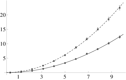
In Figs. 1–5 the numerical and analytical results for correlators (19)–(III) are presented for different time grid spacing as a function of input signal power. In Fig. 5 the results are presented for the grid spacings and because the results for and almost coincide. One can see that numerical and analytical results are in a good agreement up to 3 mW at least. However the difference between numerical and analytical results for the smallest time grid spacing is maximal. Decreasing of the parameter means the increasing of the spectral bandwidth of the noise. This increasing results in the growth of the total noise power received by detector. Note that the analytical expressions for correlators were obtained using the conditional PDF in the form (III). This form was derived in the approximation of large signal-to-noise ratio . Decreasing parameter we diminish the parameter and, as a consequence, the accuracy of our approximation. The difference between numerical and analytical results can be explained by taking into account the next-to-leading order (NLO) corrections in noise power parameter . Analytical results in Figs. 3–5 are shown with taking into account both leading order results (III)–(III) and NLO corrections presented in Appendix A, see Eqs. (A) and (A).
IV.2 Runge-Kutta method
For the equation (1) the time is the incoming parameter. Thus the simulation consists in the solution of ordinary differential equation with various initial conditions determined by the real pulse shape , the amplitude , and independent random noise functions . In the second method we used pulse envelopes of the form
| (38) |
for , : and . We choose the time discretization parameter . The random noise was realized as the telegraph process with the step of the length and of the random height with zero average and with the dispersion both for real and imaginary parts. The noise power parameter reads as W/(kmHz) and it is almost six times greater than that in the previous method. We independently control this parameter by using the leading order contribution to the correlator (III) numerically simulated for . The noise is constant within the step. Within the step the equation (1) was solved by the Runge-Kutta method of the fourth order with the step . The recovered input signal was calculated using Eq. (11) at the equidistant points . The coefficients were calculated using Eq. (12). The average (19) and correlators (III),(III) were calculated over 16384 values of which were found for various noise realizations.
To control the accuracy of the method we solved the equation (1) with zero noise from to with the step and then we performed the backward propagation from to with the found solution as the initial condition. In the procedure the input signal was recovered with the relative precision equal to .
The analytical results in comparison with the numerical results are presented in Figs. 6–10 for different pulse shapes and average power. The numerical results are presented with statistic errors on the level of three standard deviations. One can see that numerical and analytical results are in a good agreement as well.


V Entropies and mutual information
Now we proceed to the calculation of the output signal entropy
| (39) |
conditional entropy
| (40) | |||||
and the mutual information
| (41) |
Our calculations of the entropies (39), (40), and the mutual information (41) are similar to calculations of the entropies and the mutual information for per-sample channel, see Sec.III and Sec.IV of Ref. Terekhov:2016a. Therefore we will not repeat the similar calculations here and present only the final results:
| (42) | |||||
| (43) |
To calculate the optimal input signal distribution we calculate the mutual information substituting Eqs. (42) and (V) to Eq. (41) then we variate the mutual information over with taking into account the normalization condition (8) and the fixed average power (9). Assuming the variation of the mutual information to be zero, we obtain the equation for the optimal input signal distribution . We solve the equation and obtain (for details of the similar calculations for per-sample channel see the Sec.III of Ref. Terekhov:2016a):
| (44) |
where parameters and are functions of the power and modified nonlinearity parameter by virtue of the relations (compare with Eqs. (46) and (47) of Ref. Terekhov:2016a):
| (45) |
| (46) |
The capacity of one channel , i.e., the mutual information calculated using the optimal input signal distribution (44) reads
| (47) |
One can see that the first term in the right-hand side of Eq. (47) corresponds to the Shannon’s result Shannon:1948 for the linear channel at large signal-to-noise ratio, the second and third terms are related with the nonlinearity impact. The result (47) is similar to that obtained for the per-sample model in Ref. Terekhov:2016a but with modification of the Kerr nonlinearity parameter for per-sample model to parameter for the present model, where . There is no simple analytical form for and , see the Secs. III and IV of Ref. Terekhov:2016a, therefore we present below the analytical results for the asymptotics of the mutual information for small and large dimensionless nonlinearity parameter and the numerical calculations in Fig. 11.

Performing the substitution in the results of the Sec.III and Sec IV of Ref. Terekhov:2016a we arrive at following asymptotics of the mutual information for small and large dimensionless nonlinearity parameter :
| (48) |
for , and
| (49) |
for and . Here , is the Euler constant. Note that the asymptotics (V) is obtained with accuracy , see the Sec. IV of Ref. Terekhov:2016a.
VI Conclusion
In the present paper we use results obtained in Ref. Terekhov:2016a for per-sample model to calculate the informational characteristics of the channel where the input signal depends on time, see Eq. (6). For this channel the information is carried by coefficients . In the process of the signal propagation the input signal is transformed by the Kerr nonlinearity and the noise in the channel. To recover the transmitted information we introduce the detection procedure which removes the nonlinearity effects, see Eq. (11), and then projects on the basis functions, see Eq. (12), to obtain the coefficients . Using the conditional probability density function for per-sample model obtained in Ref. Terekhov:2016a we calculate the correlators of the coefficients , see Eqs. (19)–(III). We demonstrate that these correlators depend on the noise bandwidth parameter . We also perform the numerical calculations of these correlators using two different methods and show that the numerical and analytical results are in agreement. Using obtained results for correlators we find the conditional probability density function in the leading and next-to-leading orders in parameter . Then we calculate the informational entropies and the mutual information for the channel in leading order in the parameter . We perform variation of the mutual information over the input signal distribution function and obtain the optimal input signal distribution function which maximizes the mutual information. We calculate the channel capacity in the leading order in parameter and demonstrate that the capacity depends on the pulse envelope through one parameter , see Eq. (28). The capacity grows as for sufficiently large average power : . Note that the same asymptotics was obtained for per-sample model, therefore taking into account the time dependance of the pulse envelope does not change the asymptotics behavior and modifies only the nonlinearity parameter to .
Acknowledgements.
AcknowledgmentAll authors would like to thank the Russian Science Foundation (RSF), grant No. 16-11-10133. Also A.V. would like to thank the Russian Foundation for Basic Research (RFBR), grant No. 16-31-60031. Also I.S. would like to thank the Russian Science Foundation (RSF), grant No. 17-72-30006, and Ministry of Education and Science of the Russian Federation (14.Y26.31.0017).
Appendix A Correlators (III) and (III) with NLO corrections
Let us present the correlator (III) with next-to-leading (NLO) corrections in the noise power.
| (50) |
Here we have used the relation
| (51) |
the result (19) for and the calculation of on the base of next-to-leading order result for in Ref. Terekhov:2017.
In a similar manner it is easy to calculate the following corrections to correlator (III) from the results obtained in Ref. Terekhov:2017:
| (52) |
Note that these NLO results (A) and (A) contain the time discretization parameter related with the noise bandwidth . The relative importance of the NLO corrections in correlators (A) and (A) is governed by the dimensionless parameter , i.e., it increases linearly for large and increasing . To demonstrate the importance of these corrections for our numerical results we present the Fig. (12) where for the noise power parameter W/(kmHz) the imaginary part of the leading order contribution (III) and the next-to-leading order corrections (A) are presented together with the numerical results (Runge-Kutta method) for the envelope form . One can see that our calculations, i.e., Eq. (24) and formulae of the Sec. V based on the leading order results (19)–(III) are in a good agreement with the numerical calculations up to the average power of order of 4 mW for given noise and channel parameters.

References
- (1) I. S. Terekhov, A. V. Reznichenko, Ya. A. Kharkov, and S. K. Turitsyn, Phys. Rev. E 95, 062133 (2017).
- (2) A. A. Panarin, A. V. Reznichenko, I. S. Terekhov, Phys. Rev. E 95, 012127 (2016).
- (3) P. P. Mitra and J. B. Stark, Nature 411, 1027 (2001).
- (4) E. E. Narimanov and P. Mitra, J. Lightwave Technol. 20, 530 (2002).
- (5) J. M. Kahn and K.-P. Ho, IEEE. J. Sel. Topics Quant. Electron. 10, 259 (2004).
- (6) R.-J. Essiambre, G. J. Foschini, G. Kramer, and P. J. Winzer, Phys. Rev. Lett. 101, 163901 (2008).
- (7) R.-J. Essiambre, G. Kramer, P. J. Winzer, G. J. Foschini, and B. Goebel, J. of Lightwave Technol. 28, 662 (2010).
- (8) R. Killey and C. Behrens, J. Mod. Opt. 58, 1 (2011).
- (9) E. Agrell, A. Alvarado, G. Durisi, and M. Karlsson, IEEE/OSA J. Lightwave Technol. 32, 2862 (2014).
- (10) M. A. Sorokina and S. K. Turitsyn, Nat. Comm. 5, 3861 (2014).
- (11) I. S. Terekhov, A. V. Reznichenko, and S. K. Turitsyn, Phys. Rev. E, 94, 042203 (2016).
- (12) A. Mecozzi, J. Lightwave Technol. 12, 1993 (1994).
- (13) K.S. Turitsyn, S.A. Derevyanko, I.V. Yurkevich, and S.K. Turitsyn, Phys. Rev. Lett. 91, 203901 (2003).
- (14) M. I. Yousefi and F. R. Kschischang, IEEE Trans. on Information Theory 57, 7522 (2011).
- (15) G. Kramer, Submitted to the IEEE Transactions on Information Theory, (2018) arXiv:1705.00454v2.
- (16) M. A. Lavrentiev and B. V. Shabat, Method of Complex Function Theory. (Nauka, Moscow, 1987, in Russian); M. Lavrentiev and B. Chabot, Methodes de la Theorie des fonctions d’une variable complexe (Mir, Moscou, 1977, in French).
- (17) G. P. Agrawal, Nonlinear Fiber Optics (Academic press, 4th edition, 2007).
- (18) R. H. Hardin and F. D. Tappert, SIAM Rev. Chronicle, 15, 423 (1973).
- (19) C. Shannon, Bell Syst. Tech. J. 27, 379 (1948); 27, 623 (1948).