Distributed linear regression by averaging
Abstract
Distributed statistical learning problems arise commonly when dealing with large datasets. In this setup, datasets are partitioned over machines, which compute locally, and communicate short messages. Communication is often the bottleneck. In this paper, we study one-step and iterative weighted parameter averaging in statistical linear models under data parallelism. We do linear regression on each machine, send the results to a central server, and take a weighted average of the parameters. Optionally, we iterate, sending back the weighted average and doing local ridge regressions centered at it. How does this work compared to doing linear regression on the full data? Here we study the performance loss in estimation, test error, and confidence interval length in high dimensions, where the number of parameters is comparable to the training data size.
We find the performance loss in one-step weighted averaging, and also give results for iterative averaging. We also find that different problems are affected differently by the distributed framework. Estimation error and confidence interval length increase a lot, while prediction error increases much less. We rely on recent results from random matrix theory, where we develop a new calculus of deterministic equivalents as a tool of broader interest.
1 Introduction

Datasets are constantly increasing in size and complexity. This leads to important challenges for practitioners. Statistical inference and machine learning, which used to be computationally convenient on small datasets, now bring an enormous computational burden.
Distributed computation is a universal approach to deal with large datasets. Datasets are partitioned across several machines (or workers). The machines perform computations locally and communicate only small bits of information with each other. They coordinate to compute the desired quantity. This is the standard approach taken at large technology companies, which routinely deal with huge datasets spread over computing units. What are the best ways to divide up and coordinate the work?
The same problem arises when the data is distributed due to privacy, security, or ethical concerns. For instance, medical and healthcare data is typically distributed across hospitals or medical units. The parties agree that they want to aggregate the results. At the same time, they do not want other parties access their data. How can they compute the desired aggregates, without sharing the data?
In both cases, the key question is how to do statistical estimation and machine learning in a distributed setting. And what performance can the best methods achieve? This is a question of broad interest, and it is expected that the area of distributed estimation and computation will grow even more in the future.
In this paper, we develop precise theoretical answers to fundamental questions in distributed estimation. We study one-step and iterative parameter averaging in statistical linear models under data parallelism. Specifically, suppose in the simplest case that we do linear regression (Ordinary Least Squares, OLS) on each subset of a dataset distributed over machines, and take an optimal weighted average of the regression coefficients. How do the statistical and predictive properties of this estimator compare to doing OLS on the full data?
We study the behavior of several learning and inference problems, such as estimation error, test error (i.e., out-of-sample prediction error), and confidence intervals. We also consider a high-dimensional (or proportional-limit) setting where the number of parameters is of the same order as the number of total samples (i.e., the size of the training data). We also study an analogous iterative algorithm, where we do local ridge regressions, take averages of the parameters on a central machine, send back the update to the local machines, and then again do local ridge, but where the penalty is centered around the previous mean. Our iterative algorithm falls between several classical methods such as ADMM and DANE, and we discuss connections.
We discover the following key phenomena, some of which are surprising in the context of existing work:
- 1.
Sub-optimality. One-step averaging is not optimal (even with optimal weights), meaning that it leads to a performance decay. In contrast to some recent work (see the related work section), we find that there is a clear performance loss due to one-step averaging even if we split the data only into two subsets. This loss is because the number of parameters is of the same order as the sample size. However, we can quantify this loss precisely.
- 2.
Strong problem-dependence. Different learning and inference problems are affected differently by the distributed framework. Specifically, estimation error and the length of confidence intervals increases a lot, while prediction error increases less. The intuition is that prediction is a noisy task, and hence the extra error incurred is relatively smaller.
- 3.
Simple form and universality. The asymptotic efficiencies for one step distributed learning have simple forms that are often universal. Specifically, they do not depend on the covariance matrix of the data, or on the sample sizes on the local machines. For instance, the estimation efficiency decreases linearly in the number of machines (see Figure 1 and Table 1).
- 4.
Iterative parameter averaging has benefits. We show that simple iterative parameter averaging mechanisms can reduce the error efficiently. We also exhibit computation-statistics tradeoffs: depending on the hyperparameters, we can converge fast to statistically suboptimal solutions; or vice versa.
While there is already a lot of work in this direction (see Section 2) our results are new and complementary. The key elements of novelty of our setting are: (1) The sample size and the dimension are comparable, and we do not assume sparsity. (2) We have a new mathematical approach, using recent results from asymptotic random matrix theory such as (Rubio and Mestre 2011). Our approach also develops a novel theoretical tool, the calculus of deterministic equivalents, and we illustrate how it can be useful in other problems as well. (3) We consider several accuracy metrics (estimation, prediction) in a unified framework of so-called general linear functionals.
| Quantity | Relative efficiency () |
|---|---|
| Estimation & CIs | |
| Test error |
The code for our paper is available at http://www.github.com/dobriban/dist.
2 Some related work
In this section we discuss some related work. There is a great deal of work in computer science and optimization on parallel and distributed computation (Bertsekas and Tsitsiklis 1989; Boyd et al. 2011; Bekkerman et al. 2011, see e.g.,). In addition, there are several popular examples of distributed data processing frameworks: for instance MapReduce (Dean and Ghemawat 2008) and Spark (Zaharia et al. 2010).
In contrast, there is less work on understanding the statistical properties, and the inherent computation-statistics tradeoffs, in distributed computation environments. This area has attracted increasing attention only in recent years, see for instance Mcdonald et al. 2009; Zhang et al. 2012; Zhang et al. 2013b; Zhang et al. 2013a; Duchi et al. 2014; Zhang et al. 2015; Braverman et al. 2016; Jordan et al. 2016; Rosenblatt and Nadler 2016; Smith et al. 2016; Fan et al. 2017; Lin et al. 2017; Lee et al. 2017; Battey et al. 2018; Zhu and Lafferty 2018, and the references therein. See Huo and Cao 2018 for a review. We can only discuss the most closely related papers due to space limitations.
Zinkevich et al. 2009 study the parallelization of SGD for learning, by reducing it to the study of delayed SGD; giving positive results for low latency ”multicore” settings. They give an insightful discussion of the impact of various computational platforms, such as shared memory architectures, clusters, and grid computing. Mcdonald et al. 2009 propose averaging methods for special conditional maximum entropy models, showing variance reduction properties. Zinkevich et al. 2010 expand on this, proposing ”parallel SGD” to average the SGD iterates computed on random subsets of the data. Their proof is based on the contraction properties of SGD.
Zhang et al. 2013b bound the leading order term for MSE of averaged estimation in empirical risk minimization. Their bounds do not explicitly take dimension into account. However, their empirical data example clearly has large dimension , considering a logistic regression with sample size , and , so that . In their experiments, they distribute the data over up to 128 machines. So, our regime, where is of the same order as , matches well their simulation setup. In addition, their concern is on regularized estimators, where they propose to estimate and reduce bias by subsampling.
Liu and Ihler 2014 study distributed estimation in statistical exponential families, connecting the efficiency loss from the global setting to the deviation from full exponential families. They also propose nonlinear KL-divergence-based combination methods, which can be more efficient than linear averaging.
Zhang et al. 2015 study divide and conquer kernel ridge regression, showing that the partition-based estimator achieves the statistical minimax rate over all estimators. Due to their generality, their results are more involved, and also their dimension is fixed. Lin et al. 2017 improve those results. Duchi et al. 2014 derive minimax bounds on distributed estimation where the number of bits communicated is controlled.
Rosenblatt and Nadler 2016 consider the distributed learning problem in three different settings. The first two settings are fixed dimensional. The third setting is high-dimensional M-estimation, where they study the first order behavior of estimators using prior results from Donoho and Montanari 2013; El Karoui et al. 2013. This is possibly the most closely related work to ours in the literature. They use the following representation, derived in the previous works mentioned above: a high-dimensional -estimator can be written as , where , is the limit of , and is a constant depending on the loss function, whose expression can be found in Donoho and Montanari 2013; El Karoui et al. 2013.
They derive a relative efficiency formula in this setting, which for OLS takes the form
In contrast, our result for this case (Theorem 5.1) is equal to
Thus, our result is much more precise, and in fact exact, while of course being limited to the special case of linear regression.
In a heterogeneous data setting, Zhao et al. 2016 fit partially linear models, and estimate the common part by averaging. For model selection problems in GLM, Chen and Xie 2014 propose weighted majority voting methods. Lee et al. 2017 study sparse linear regression, showing that averaging debiased lasso estimators can achieve the optimal estimation rate if the number of machines is not too large. Battey et al. 2018 study a similar problem, also including hypothesis testing under more general sparse models. Shi et al. 2018; Banerjee et al. 2019 show that in problems with non-standard rates, averaging can lead to improved pointwise inference, while decreasing performance in a uniform sense. Volgushev et al. 2019 (among other contributions) provide conditions under which averaging quantile regression estimators have an optimal rate. Banerjee and Durot 2018 propose improvements based on communicating smoothed data, and fitting estimators after. Szabo and van Zanten 2018 study estimation methods under communication constraints in nonparametric random design regression model, deriving both minimax lower bounds and optimal methods.
See Section 7 for more discussion of multi-round methods.
3 One-step weighted averaging: General linear functionals
We consider the standard linear model
Here we have an outcome variable along with some covariates , and want to understand their relationship. We observe such data points, arranging their outcomes into the vector , and their covariates into the matrix . We assume that depends linearly on , via some unknown parameter vector .
We assume there are more samples than training data points, i.e., , while can also be large. In that case, a gold standard is the usual least squares estimator (ordinary least squares or OLS)
We also assume that the coordinates of the noise are uncorrelated and have variance .
Suppose now that the samples are distributed across machines (these can be real machines, but they can also be—say—sites or hospitals in medical applications, or mobile devices in federated learning). The -th machine has the matrix , containing samples, and also the vector of the corresponding outcomes for those samples. Thus, the -th worker has access to only a subset of training data points out of the total of training data points. For instance, if the data points denote users, then they may be partitioned into sets based on country of residence, and we may have samples from the United States on one server, samples from Canada on another server, etc. The broad question is: How can we estimate the unknown regression parameter if we need to do most of the computations locally?
Let us write the partitioned data as
We also assume that each local OLS estimator is well defined, which requires that the number of local training data points must be at least on each machine (so ). We first consider combining the local OLS estimators at a parameter server via one-step weighted averaging. Since they are uncorrelated and unbiased for , we consider unbiased weighted estimators
with .
We introduce a ”general linear functional” framework to study learning tasks such as estimation and prediction in a unified way. In the general framework, we predict linear functionals of of the form
Here is a fixed matrix, and is a zero-mean Gaussian noise vector of dimension , with covariance matrix , for some scalar parameter . We denote the covariance matrix between and by , so that . If , we say that there is no noise. In that case, we necessarily have .
We predict the linear functional via plug-in based on some estimator (typically OLS or distributed OLS)
We measure the quality of estimation by the mean squared error
We compute the relative efficiency of OLS compared to a weighted distributed estimator :
The relative efficiency is a fundamental quantity, giving the loss of accuracy due to distributed estimation.
3.1 Examples
We now show how several learning and inference problems fall into the general framework. See Table 2 for a concise summary.
| Statistical learning problem | |||||
| Estimation | 0 | 0 | |||
| Regression function estimation | 0 | 0 | |||
| Confidence interval | 0 | 0 | |||
| Test error | 1 | 0 | |||
| Training error |
- •
Parameter estimation. In parameter estimation, we want to estimate the regression coefficient vector using . This is an example of the general framework by taking , and without noise (so that ).
- •
Regression function estimation. We can use to estimate the regression function . In this case, the transform matrix is , the linear functional is , the predictor is , and there is no noise.
- •
Out-of-sample prediction (Test error). For out-of-sample prediction, or test error, we consider a test data point , generated from the same model , where are independent of , and only is observable. We want to use to predict .
This corresponds to predicting the linear functional , so that , and the noise is , which is uncorrelated with the noise in the original problem.
- •
In-sample prediction (Training error). For in-sample prediction, or training error, we consider predicting the response vector , using the model fit . Therefore, the functional is This agrees with regression function estimation, except for the noise , which is identical to the original noise. Hence, the noise scale is , and .
- •
Confidence intervals. To construct confidence intervals for individual coordinates, we consider the normal model . Assuming is known, a confidence interval with coverage for a given coordinate is
where is the inverse normal CDF, and is the -th diagonal entry of .
Therefore, we can measure the difficulty of the problem by . The larger is, the longer the confidence interval. This also measures the difficulty of estimating the coordinate . This can be fit in our general framework by choosing , the vector of zeros, with only a one in the -th coordinate. This problem is noiseless. In this sense, the problem of confidence intervals is the same as the estimation accuracy for individual coordinates of .
If is not known, then we we first need to estimate it in a distributed way. This is an interesting problem in itself, but beyond the scope of our current work.
3.2 Finite sample results
We now show how to calculate the efficiency explicitly in the general framework. We start with the simpler case where . We then have for the OLS estimator
For the distributed estimator with weights summing to one, given by , we have
Using a simple Cauchy-Schwarz inequality (see Section A for the argument for parameter estimation), we find that the optimal efficiency, for the optimal weights, is
| (1) |
This shows that the key to understanding the efficiency are the traces Proving that the efficiency is at most unity turns out to require the concavity of the matrix functional . This is a consequence of classical results in convex analysis, see for instance Davis 1957; Lewis 1996. For completeness, we give a short self-contained proof in Section B of the Appendix.
Proposition 3.1 (Concavity for general efficiency, Davis 1957; Lewis 1996).
The function is a concave function defined on positive definite matrices. As a consequence, the general relative efficiency for distributed estimation is at most unity for any matrices :
For the more general case when , we can also find the OLS MSE as
For the distributed estimator, we can find, denoting ,
Let , and . The optimal weights can be found from a quadratic optimization problem:
The resulting formula for the optimal weights, and for the global optimum, can be calculated explicitly. The details can be found in the supplement (Section C).
4 Calculus of deterministic equivalents
4.1 A calculus of deterministic equivalents in RMT
We saw that the relative efficiency depends on the trace functionals , for specific matrices . To find their limits, we will use the technique of deterministic equivalents from random matrix theory. This is a method to find the almost sure limits of random quantities. See for example Hachem et al. 2007; Couillet et al. 2011 and the related work section below.
For instance, the well known Marchenko-Pastur (MP) law for the eigenvalues of random matrices (Marchenko and Pastur 1967; Bai and Silverstein 2009) states that the eigenvalue distribution of certain random matrices is asymptotically deterministic. More generally, one of the best ways to understand the MP law is that resolvents are asymptotically deterministic. Indeed, let , where and is a random matrix with iid entries of zero mean and unit variance. Then the MP law means that for any with positive imaginary part, we have the equivalence
for a certain scalar (that will be specified later). At this stage we can think of the equivalence entry-wise, but we will make this precise next. The above formulation has appeared in some early works by VI Serdobolskii, see e.g., Serdobolskii 1983, and Theorem 1 on page 15 of Serdobolskii 2007 for a very clear statement.
The consequence is that simple linear functionals of the random matrix have a deterministic equivalent based on . In particular, we can approximate the needed trace functionals by simpler deterministic quantities. For this we will take a principled approach and define some appropriate notions for a calculus of deterministic equivalents, which allows us to do calculations in a simple and effective way.
First, we make more precise the notion of equivalence. We say that the (deterministic or random) not necessarily symmetric matrix sequences of growing dimensions are equivalent, and write
if
almost surely, for any sequence of not necessarily symmetric matrices with bounded trace norm, i.e., such that
We call such a sequence a standard sequence. Recall here that the trace norm (or nuclear norm) is defined by , where are the singular values of .
4.2 General MP theorem
To find the limits of the efficiencies, the most important deterministic equivalent will be the following result, essentially a consequence of the generalized Marchenko-Pastur theorem of Rubio and Mestre 2011 (see Section D for the argument). We study the more general setting of elliptical data. In this model the data samples may have different scalings, having the form , for some vector with iid entries, and for datapoint-specific scale parameters . Arranging the data as the rows of the matrix , that takes the form
where and are as before: has iid standardized entries, while is the covariance matrix of the features. Now is the diagonal scaling matrix containing the scales of the samples. This model has a long history in multivariate statistics (Mardia et al. 1979, e.g.,).
Theorem 4.1 (Deterministic equivalent in elliptical models, consequence of Rubio and Mestre 2011).
Let the data matrix follow the elliptical model
where is an diagonal matrix with non-negative entries representing the scales of the observations, and is a positive definite matrix representing the covariance matrix of the features. Assume the following:
- 1.
The entries of are iid random variables with mean zero, unit variance, and finite -th moment, for some .
- 2.
The eigenvalues of , and the entries of , are uniformly bounded away from zero and infinity.
- 3.
We have , with bounded away from zero and infinity.
Let be the sample covariance matrix. Then is equivalent to a scaled version of the population covariance
Here is the unique solution of the fixed-point equation
Thus, the inverse sample covariance matrix has a deterministic equivalent in terms of a scaled version of the inverse population covariance matrix. This result does not require the convergence of the aspect ratio , or of the e.s.d. of , and , as is sometimes the case in random matrix theory. However, if the empirical spectral distribution of the scales tends to , the above equation has the limit
The usual MP theorem is a special case of the above result where . As a result, we obtain the following corollary:
Corollary 4.2 (Deterministic equivalent in MP models).
Let the data matrix follow the model where is a positive definite matrix representing the covariance matrix of the features. Assume the same conditions on from Theorem 4.1. Then is equivalent to a scaled version of the population covariance
The proof is immediate, by checking that in this case.
4.2.1 Related work on deterministic equivalents
There are several works in random matrix theory on deterministic equivalents. One of the early works is Serdobolskii 1983, see Serdobolskii 2007 for a modern summary. The name ”deterministic equivalents” and technique was more recently introduced and re-popularized by Hachem et al. 2007 for signal-plus-noise matrices. Later Couillet et al. 2011 developed deterministic equivalents for matrix models of the type , motivated by wireless communications. See the book Couillet and Debbah 2011 for a summary of related work. See also Müller and Debbah 2016 for a tutorial. However, many of these results are stated only for some fixed functional of the resolvent, such as the Stieltjes transform. One of our points here is that there is a much more general picture.
Rubio and Mestre 2011 is one of the few works that explicitly states more general convergence of arbitrary trace functionals of the resolvent. Our results are essentially a consequence of theirs.
However, we think that it is valuable to define a set of rules, a ”calculus” for working with deterministic equivalents, and we use those techniques in our paper. Similar ideas for operations on deterministic equivalents have appeared in Peacock et al. 2008, for the specific case of a matrix product. Our approach is more general, and allows many more matrix operations, see below.
4.3 Rules of calculus
The calculus of deterministic equivalents has several properties that simplify calculations. We think these justify the name of calculus. Below, we will denote by etc, sequences of deterministic or random matrices. See Section E in the supplement for the proof.
Theorem 4.3 (Rules of calculus).
The calculus of deterministic equivalents has the following properties.
- 1.
Equivalence. The relation is indeed an equivalence relation.
- 2.
Sum. If and , then .
- 3.
Product. If is a sequence of matrices with bounded operator norms i.e., , and , then .
- 4.
Trace. If , then almost surely.
- 5.
Stieltjes transforms. As a consequence, if for symmetric matrices , then almost surely. Here is the Stieltjes transform of the empirical spectral distribution of .
In addition, the calculus of deterministic equivalents has additional properties, such as continuous mapping theorems, differentiability, etc. We have developed the differentiability in the follow-up work (Dobriban and Sheng 2019).
We also briefly sketch several applications of the calculus of deterministic equivalents in Section F in the supplement, to studying the risk of ridge regression in high dimensions, including in the distributed setting, gradient flow for least squares, interpolation in high dimensions, heteroskedastic PCA, as well as exponential family PCA. We emphasize that in each case, including for the formulas of asymptotic efficiencies in the current work, there are other proof techniques, but they tend to be more case-by-case. The calculus provides a unified set of methods, and separate results can be seen as applications of the same approach.
5 Examples
We now use the calculus of deterministic equivalents to find the limits of the trace functionals in our general framework. We study each problem in turn. For asymptotics, we consider as before elliptical models. The data on the -th machine takes the form
where contains the scales of the -th machine and is the appropriate submatrix of .
In this model, it turns out that the efficiencies can be expressed in a simple way via the -transform (Tulino and Verdú 2004). The -transform of a distribution is
for all for which this expectation is well-defined. We will see that the efficiencies can be expressed in terms of the functional inverse of the -transform evaluated at the specific value :
| (2) |
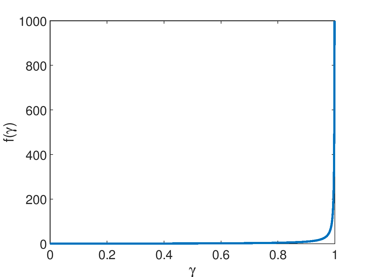
We think of elliptical models where the limiting distribution of the scales is . For some insight on the behavior of and , consider first the case when is a point mass at unity, . In this case, all scales are equal, so this is just the usual Marchenko-Pastur model. Then, we have , while . See Figure 2 for the plots. The key points to notice are that is a decreasing function of , with , and . Moreover, is an increasing function on with , . The same qualitative properties hold in general for compactly supported distributions bounded away from .

5.1 Parameter estimation
For estimating the parameter, we have . We find via (1) the estimation efficiency
Recall that . Recall that the empirical spectral distribution (e.s.d.) of a symmetric matrix is simply the CDF of its eigenvalues (which are all real-valued). More formally, it is the discrete distribution that places equal mass on all eigenvalues of .
Theorem 5.1 (RE for elliptical and MP models).
Under the conditions of Theorem 4.1, suppose that, as with , the of converges weakly to some , the of each converges weakly to some , and that the of converges weakly to . Suppose that is compactly supported away from the origin, while is also compactly supported and does not have a point mass at the origin. Then, the RE has almost sure limit
For Marchenko-Pastur models, the RE has the form
See Section G in the supplement for the proof. For MP models, for any finite sample size , dimension , and number of machines , we can approximate the ARE as
This efficiency for MP models depends on a simple linear way on . We find this to be a surprisingly simple formula, which can also be easily computed in practice. Moreover, the formula has several more intriguing properties:
- 1.
The ARE decreases linearly with the number of machines . This holds as long as . At the threshold case , there is a phase transition. The reason is that there is a singularity, and the OLS estimator is undefined for at least one machine.
However, we should be cautious about interpreting the linear decrease. For the root mean squared error (RMSE), the efficiency is the square root of the ARE above, and thus does not have a linear decrease.
- 2.
The ARE has two important universality properties.
- (a)
First, it does not depend on how the samples are distributed across the different machines, i.e., it is independent of the specific sample sizes .
- (b)
Second, it does not depend on the covariance matrix of the samples. This is in contrast to the estimation error of OLS, which does in fact depend on the covariance structure. Therefore, we think that the cancellation of in the ARE is noteworthy.
- (a)
The ARE is also very accurate in simulations. See Figure 3 for an example. Here we report the results of a simulation where we generate an random matrix such that the rows are distributed independently as . We take to be diagonal with entries chosen uniformly at random between 1 and 2. We choose , and for each value of such that , we split the data into groups of a random size . To ensure that each group has a size , we first let , and then distribute the remaining samples uniformly at random. We then show the theoretical results compared to the theoretical ARE. We observe that the two agree closely.


5.2 Regression function estimation
For estimating the regression function, we have . We then find via equation (1) the prediction efficiency
For asymptotics, we consider as before elliptical models.
Theorem 5.2 (FE for elliptical and MP models).
See Section G.6 for the proof. This efficiency is more complex than that for estimation error; specifically it generally depends on the individual and not just .
5.3 In-sample prediction (Training error)
For in-sample prediction, we start with the well known formula
As we saw, to fit in-sample prediction in the general framework, we need to take the transform matrix , the noise , and the covariance matrices . Then, in the formula for optimal weights we need to take and . Therefore, the optimal error for distributed regression is achieved by the weights
Plugging these into given in the general framework, we find
Thus, the optimal in-sample prediction efficiency is
For asymptotics in elliptical models, we find:
Theorem 5.3 (IE for elliptical and MP models).
See Section G.7 for the proof. This efficiency does not depend on a simple linear way on , but rather via a ratio of two linear functions of . However, it can be checked that many of the properties (e.g., monotonicity) for ARE still hold here.
5.4 Out-of-sample prediction (Test error)
In out-of-sample prediction, we consider a test datapoint , generated from the same model , where are independent of , and only is observable. We want to use to predict . We compare the prediction error of two estimators:
In our general framework, we saw that this corresponds to predicting the linear functional . Based on equation (1), the optimal out-of-sample prediction efficiency is
For asymptotics in elliptical models, we find the following result. Since the samples have the form , the test sample depends on a scale parameter .
Theorem 5.4 (OE for elliptical and MP models).
See Section G.8 for the proof. If the scale parameter is random, then the OE typically does not have an almost sure limit, and converges in distribution to a random variable instead. We mention that Theorem 5.4 holds under even weaker conditions, if we are only given the -th moment of instead of -th one. The argument is slightly different, and is presented in the location referenced above.
One can check that that . Thus, out-of-sample prediction incurs a smaller efficiency loss than estimation. The intuition is that the out-of-sample prediction always involves a fixed loss due to the irreducible noise in the test sample, which ”amortizes” the problem. Moreover,
The intuition here is that IE incurs a smaller fixed loss than OE, because the noise in the training set is effectively reduced, as it is already partly fit by our estimation process. So the graph of IE will be in between the other two criteria. See Figure 4. We also see that the IE is typically very close to OE.
In addition, the increase of the reducible part of the error is the same as for estimation error. The prediction error has two components: the irreducible noise, and the reducible error. The reducible error has the same behavior as for estimation, and thus on figure 4 it would have the same plot as the curve for estimation.
5.5 Confidence intervals
To form confidence intervals, we consider the normal model . Recall that in this model the OLS estimator has distribution Assuming is known, an exact level confidence interval for a given coordinate can be formed as
where is the inverse normal CDF, and is the -th diagonal entry of . We follow the same program as before, comparing the length of the confidence intervals formed based on our two estimators. However, for technical reasons it is more convenient to work with squared length.
Thus we consider the criterion
Here is the variance of the -th entry of an optimally weighted distributed estimator. As we saw in our framework, this is equivalent to estimating the -th coordinate of . Hence the optimal confidence interval efficiency is
| (3) |
For asymptotics, we find:
Theorem 5.5 (CE for elliptical and MP models).
See Section G.9 for the proof.
5.6 Understanding and comparing the efficiencies
We give two perspectives for understanding and comparing the efficiencies. The key qualitative insight is that estimation and CIs are much more affected than prediction.
Criticality of . We ask: What is the largest number of machines such that the asymptotic efficiency is at least 1/2? Let us call this the critical number of machines. It is easy to check that for estimation and CIs, . For training error, , while for test error, .
We also have the following asymptotics as :
while
So the number of machines that can be used is nearly maximal (i.e., ) for training and test error, while it is about half that for estimation error and CIs. This shows quantitatively that estimation and CIs are much more affected by distributed averaging than prediction.
Edge efficiency. The maximum number of machines that we can use is approximately , for small . Let us define the edge efficiency as the relative efficiency achieved at this edge case. For estimation and CIs, we have . For training error, , and for test error, .
We also have the following asymptotic values as :
while
This shows that for the edge efficiency is vanishing for estimation and CIs, while it is approximately 1/2 for training and test error. Thus, even for the maximal number of machines, prediction error is not greatly increased.
6 Insights for Parameter Estimation
There are additional insights for the special case of parameter estimation. First, it is of interest to understand the performance of one-step weighted averaging with suboptimal weights . How much do we lose compared to the optimal performance if we do not use the right weights? In practice, it may seem reasonable to take a simple average of all estimators. We have performed that analysis in the supplement (Section H.1), and we found that the loss can be viewed in terms of an inequality between the arithmetic and harmonic means.
There are several more remarkable properties. We have studied the monotonicity properties and interpretation of the relative efficiency, see the supplement (Section H.2). We have also given a multi-response regression characterization that heuristically gives an upper bound on the ”degrees of freedom” for distributed regression (Section H.3).
For elliptical data, the graph of ARE is a curve below the straight line from before. The interpretation is that for elliptical distributions, there is a larger efficiency loss in one-step weighted averaging. Intuitively, the problem becomes ”more non-orthogonal” due to the additional variability from sample to sample.
It is natural to ask which elliptical distributions are difficult for distributed estimation. For what scale distributions does the distributed setting have a strong effect on the learning accuracy? Intuitively, if some of the scales are much larger than others, then they ”dominate” the problem, and may effectively reduce the sample size. We show that this intuition is correct, and we find a sequence of scale distributions such that distributed estimation is ”arbitrarily bad”, so that the ARE decreases very rapidly, and approaches zero even for two machines (see Section G.1 in the supplement).
7 Multi-shot methods
While our focus has been on methods with one round of communication, in practice it is more common to use iterative methods with several rounds of communication. These usually improve statistical accuracy. A great deal of research has been done on multi-shot distributed algorithms. Due to limited space, here we will only list and analyze some of them. Our least squares objective can be written as a sum of least squares objectives for each machine as
Here each machine has access only to local data . With this formulation, there are a large number of standard optimization methods to minimize this objective: distributed gradient descent, alternating directions method of multipliers, and several others we discuss below. We will focus on parameter server architectures, where each machine communicates independently with a central server.
Distributed Gradient Descent. A simple multi-round approach to distributed learning is synchronous distributed gradient descent (DGD), as discussed e.g., in Chu et al. 2007. This maintains iterates , started with some standard value, such as . At each iteration each local machine calculates the gradient at the current iterate , and then sends the local gradient to the server to obtain the overall gradient
Then the center server sends the updated parameter back to the local machines, where is the learning rate (LR). This synchronous implementation is identical to centralized gradient descent. Thus for smooth and strongly convex objectives and suitably small , communication rounds are sufficient to attain an -suboptimal solution in terms of objective value, where are the smoothness and strong convexity parameters (Boyd and Vandenberghe 2004, e.g.,).
- 1.
Many works study the optimization properties of GD/synchronous DGD, in terms of convergence rate to the optimal objective or parameter value. From a statistical point of view, the GD iterates start with large bias and small variance, and gradually reduce bias, while slightly increasing the variance. This has motivated work on the risk properties of GD, emphasizing early stopping (Yao et al. 2007; Ali et al. 2019, e.g.,). Recently, Ali et al. 2019 gave a more refined analysis of the estimation risk of GD for OLS, showing that its risk at an optimal stopping time is at most 1.22 times the risk of optimally tuned ridge regression.
- 2.
Compared to GD, one-shot weighted averaging has several advantages: it is simpler to implement, as it requires no iterations. It requires fewer tuning parameters, and those can be set optimally in an easy way, unlike the LR . The weights are proportional to , which can be computed locally. We point out that GD is sensitive to the learning rate: this has to be bounded (by for OLS) to converge, and the convergence can be faster for large LR, hence in practice sophisticated LR schedules are used. This can make DGD complicated to use. In addition, in practice DGD is susceptible to stragglers, i.e., machines that take too long to compute their answers. To mitigate this problems, asynchronous DGD algorithms (Tsitsiklis et al. 1986; Nedic and Ozdaglar 2009, e.g.,), and other sophisticated coding ideas (Tandon et al. 2017) have been proposed. However those lead to additional complexity and hyperparameters to tune (e.g., for async algorithms: how much to wait, how to aggregate non-straggler gradients).
- 3.
One may also use other gradient based methods, such as accelerated or quasi-Newton methods, e.g., L-BFGS (Agarwal et al. 2014).
Alternating Direction Method of Multipliers (ADMM). Another approach is the alternating direction method of multipliers (see Boyd et al. 2011, for an exposition) and its variants. In ADMM, we alternate between solving local problems, global averaging, and computing local dual variables. For us, at time step of ADMM, each local machine calculates a local estimator
(where is a hyperparameter) and sends it to the parameter server to get an average
Finally, the server sends back to the local machines to update the dual variables
These three steps can be written as a linear recursion for a state variable including and . If all singular values of are less than one, then the iteration converges to a fixed point solving , so that . However, it seems hard to prove convergence in our asymptotic setting.
Distributed Approximate Newton-type Method (DANE). Shamir et al. 2014 proposed an approximate Newton-like method (DANE), which uses that the sub-problems are similar. For our problem, DANE aggregates the local gradients on the parameter server at each step , and sends this quantity, i.e., to all machines. Then each machine computes a local estimator by a gradient step in the direction of a regularized local Hessian ,
where is the regularizer and is the learning rate. The machines send it to the server to get the aggregated estimator
For a noiseless model where , we can summarize the update rule as
so we have the error bound
In Shamir et al. 2014, the authors showed that given a suitable learning rate and regularizer , when is close to , as .
For a noisy linear model , the limit of is exactly the OLS estimator of the whole data set, and we have the following recursion formula
and the convergence guarantee is the same as for the noiseless case.
Iterative Averaging Method. Here we describe an iterative averaging method for distributed linear regression. This method turns out to be connected to DANE, and it has the advantage that it can be analyzed more conveniently. We define a sequence of local estimates and global estimates with initialization . At the -th step we update the local estimate by the following weighted average of the local ridge regression estimator and the current global estimate
Then we average the local estimates
To understand this, let us first consider a noiseless model where . In that case, we can also write this update as a weighted average,
where
is the weight matrix of the global estimate. Propagating the iterative update to the global machine, we find a linear update rule:
where . Hence, the error is updated as
This recursion relation is very similar to the one for DANE; we just need to replace by (and in practice usually is used). The only difference is that DANE has a step where we need to collect the local gradients to get the global gradient, and then broadcast it to all local machines. Our iterative averaging method has lower communication cost.
In terms of convergence, will converge geometrically to for all , if and only if the largest eigenvalue of is strictly less than . It is not hard to see that this holds if at least one has positive eigenvalues by using the fact . When the samples are uniformly distributed, we should have , which means the convergence rates of DANE and iterative averaging should be very close. Hence, in terms of the total cost (communication and computation), our iterative averaging should compare favorably to DANE.
To summarize the noiseless case, we can formulate the following result:
Theorem 7.1 (Convergence of iterative averaging, noiseless case).
Consider the iterative averaging method described above. In the noiseless case when , we have the following: If at least one has positive eigenvalues, then the iterates converge to the true coefficients geometrically, , and:
Consider now the noisy case when with the same assumptions as in the rest of the paper. We have
where . As before, defining appropriately
so .
With noise, does not converge to OLS, but to the following quantity:
We can check that is an unbiased estimator for and
Under the conditions of Theorem 7.1, we have , and the MSE for is
How large is this MSE, and how does it depend on ?We have the following results.
Theorem 7.2 (Properties of Iterative averaging, noisy case).
Consider the iterative averaging method described above. In the noisy case when , we have the following:
- 1.
If at least one has strictly positive eigenvalues, then the iterates converge to the following limiting unbiased estimator
and the convergence is geometric
- 2.
The mean squared error of has the following form
- 3.
Suppose the samples are evenly distributed, i.e., and the regularizers are all the same . The MSE is a differentiable function of the regularizer , with derivative
where and
- 4.
is a non-increasing function on and . So for any , i.e. the MSE of the iterative averaging estimator with positive regularizer is smaller than the MSE of the one-step averaging estimator.
- 5.
When , reduces to the one-step averaging estimator with MSE
When , converges to the OLS estimator with MSE
See Section I of the supplement for the proof. The argument for monotonicity relies on Schur complements, and is quite nontrivial. From Theorem 7.2, it appears we should choose the regularizer as large as possible, since the limiting estimator will converge to the OLS estimator as . This is true for statistical accuracy. However, there is a computational tradeoff, since the convergence rate of to is slower for large .
Moreover, one may argue that reduces to the naive averaging estimator but not the optimally weighted averaging estimator when . However, we have shown in the supplement (Section H.1) that for evenly distributed samples, the MSE of the naive averaging estimator and the optimally weighted averaging estimator is asymptotically the same. Thus, there exists a regularizer such that the iterative averaging estimator has smaller MSE than the one-step weighted averaging estimator.
Other approaches. There are many other approaches to distributed learning. Dual averaging for decentralized optimization over a network (Duchi et al. 2011) builds on Nesterov’s dual averaging method (Nesterov 2009). It chooses the iterates to minimize an averaged first-order approximation to the function, regularized with a proximal function. The communication-efficient surrogate likelihood approximates the objective by an expression of the form , where is a preliminary estimator (Jordan et al. 2016; Wang et al. 2017). Chen et al. 2018b propose a related method for quantile regression. Both are related to DANE (Shamir et al. 2014).
Chen et al. 2018a study divide and conquer SGD (DC-SGD), running SGD on each machine and averaging the results. They also propose a distributed first-order Newton-type estimator starting with a preliminary estimator , of the form , where is the population Hessian. They show how to numerically estimate this efficiently, and also develop a more accurate multi-round version.
7.1 Numerical comparisons
We report simulations to compare the convergence rate and statistical accuracy of the one-shot weighted method with some popular multi-shot methods described above (Figure 5). Here we work with a linear model , where and all follow standard normal distributions. We take , and . We plot the relative efficiencies of different methods against the number of iterations.
We can see that the one-shot weighted method is good in some cases. The multi-shot methods usually need several iterations to achieve better statistical accuracy. When the communication cost is large, one-shot methods are attractive. Also, we can clearly see the computation vs accuracy tradeoff for the iterative averaging method from the plots. When the regularizer is small, the convergence is fast, but in the end the accuracy is not as good as the other multi-shot methods. On the other hand, if the regularizer is large, we have a better accuracy with slower convergence. Moreover, the widely-used multi-shot methods can require a lot of work for parameter tuning, and sometimes it is very difficult to find the optimal parameters. See Figure 6 for an example. In contrast, weighted averaging requires less tuning, making it a more attractive method.


We have performed several more numerical simulations to verify our theory, in addition to the results shown in the paper. Due to space limitations, these are presented in the supplement. In Section K, we present an empirical data example to assess the accuracy of our theoretical results for one-shot averaging. We find that they can be quite accurate.
Acknowledgments
We thank Jason D. Lee, Philip Gressman, Andreas Haeberleen, Boaz Nadler, Balasubramanian Narashiman and Ziwei Zhu for helpful discussions. We are grateful to Sifan Liu for providing an initial script for processing the empirical data. We thank John Duchi for pointing out references from convex optimization showing the concavity of the relative efficiencies (proposition 3.1). We thank Du Bing for pointing out a typo in the definition of in a previous version of the manuscript. This work was partially supported by NSF BIGDATA grant IIS 1837992.
References
- Agarwal et al. (2014) A. Agarwal, O. Chapelle, M. Dudik, and J. Langford. A reliable effective terascale linear learning system. Journal of Machine Learning Research, 15:1111–1133, 2014.
- Ali et al. (2019) A. Ali, J. Z. Kolter, and R. J. Tibshirani. A continuous-time view of early stopping for least squares regression. In Proceedings of Machine Learning Research, volume 89, pages 1370–1378, 2019.
- Bai and Silverstein (2009) Z. Bai and J. W. Silverstein. Spectral analysis of large dimensional random matrices. Springer Series in Statistics. Springer, 2009.
- Banerjee and Durot (2018) M. Banerjee and C. Durot. Removing the curse of superefficiency: an effective strategy for distributed computing in isotonic regression. arXiv preprint arXiv:1806.08542, 2018.
- Banerjee et al. (2019) M. Banerjee, C. Durot, and B. Sen. Divide and conquer in nonstandard problems and the super-efficiency phenomenon. The Annals of Statistics, 47(2):720–757, 2019.
- Battey et al. (2018) H. Battey, J. Fan, H. Liu, J. Lu, and Z. Zhu. Distributed testing and estimation under sparse high dimensional models. The Annals of Statistics, 46(3):1352–1382, 2018.
- Bekkerman et al. (2011) R. Bekkerman, M. Bilenko, and J. Langford. Scaling up machine learning: Parallel and distributed approaches. Cambridge University Press, 2011.
- Bertsekas and Tsitsiklis (1989) D. P. Bertsekas and J. N. Tsitsiklis. Parallel and distributed computation: numerical methods, volume 23. Prentice hall Englewood Cliffs, NJ, 1989.
- Boyd and Vandenberghe (2004) S. Boyd and L. Vandenberghe. Convex optimization. Cambridge university press, 2004.
- Boyd et al. (2011) S. Boyd, N. Parikh, E. Chu, B. Peleato, and J. Eckstein. Distributed optimization and statistical learning via the alternating direction method of multipliers. Foundations and Trends® in Machine learning, 3(1):1–122, 2011.
- Braverman et al. (2016) M. Braverman, A. Garg, T. Ma, H. L. Nguyen, and D. P. Woodruff. Communication lower bounds for statistical estimation problems via a distributed data processing inequality. In Proceedings of the forty-eighth annual ACM symposium on Theory of Computing, pages 1011–1020. ACM, 2016.
- Chen et al. (2018a) X. Chen, W. Liu, and Y. Zhang. First-order newton-type estimator for distributed estimation and inference. arXiv preprint arXiv:1811.11368, 2018a.
- Chen et al. (2018b) X. Chen, W. Liu, and Y. Zhang. Quantile regression under memory constraint. arXiv preprint arXiv:1810.08264, 2018b.
- Chen and Xie (2014) X. Chen and M.-g. Xie. A split-and-conquer approach for analysis of extraordinarily large data. Statistica Sinica, pages 1655–1684, 2014.
- Chu et al. (2007) C.-T. Chu, S. K. Kim, Y.-A. Lin, Y. Yu, G. Bradski, K. Olukotun, and A. Y. Ng. Map-reduce for machine learning on multicore. In Advances in neural information processing systems, pages 281–288, 2007.
- Couillet and Debbah (2011) R. Couillet and M. Debbah. Random Matrix Methods for Wireless Communications. Cambridge University Press, 2011.
- Couillet and Hachem (2014) R. Couillet and W. Hachem. Analysis of the limiting spectral measure of large random matrices of the separable covariance type. Random Matrices: Theory and Applications, 3(04):1450016, 2014.
- Couillet et al. (2011) R. Couillet, M. Debbah, and J. W. Silverstein. A deterministic equivalent for the analysis of correlated mimo multiple access channels. IEEE Trans. Inform. Theory, 57(6):3493–3514, 2011.
- Davis (1957) C. Davis. All convex invariant functions of hermitian matrices. Archiv der Mathematik, 8(4):276–278, 1957.
- Dean and Ghemawat (2008) J. Dean and S. Ghemawat. Mapreduce: simplified data processing on large clusters. Communications of the ACM, 51(1):107–113, 2008.
- Dobriban and Sheng (2019) E. Dobriban and Y. Sheng. One-shot distributed ridge regression in high dimensions. arXiv preprint arXiv:1903.09321, 2019.
- Dobriban and Wager (2018) E. Dobriban and S. Wager. High-dimensional asymptotics of prediction: Ridge regression and classification. The Annals of Statistics, 46(1):247–279, 2018.
- Dobriban et al. (2017) E. Dobriban, W. Leeb, and A. Singer. Optimal prediction in the linearly transformed spiked model. arXiv preprint arXiv:1709.03393, 2017.
- Dobriban et al. (2019) E. Dobriban, W. Leeb, and A. Singer. Theoretical justification for exponential family pca. forthcoming, 2019.
- Donoho and Montanari (2013) D. L. Donoho and A. Montanari. High dimensional robust M-estimation: Asymptotic variance via approximate message passing. arXiv preprint arXiv:1310.7320, 2013.
- Duchi et al. (2011) J. C. Duchi, A. Agarwal, and M. J. Wainwright. Dual averaging for distributed optimization: Convergence analysis and network scaling. IEEE Transactions on Automatic control, 57(3):592–606, 2011.
- Duchi et al. (2014) J. C. Duchi, M. I. Jordan, M. J. Wainwright, and Y. Zhang. Optimality guarantees for distributed statistical estimation. arXiv preprint arXiv:1405.0782, 2014.
- El Karoui et al. (2013) N. El Karoui, D. Bean, P. J. Bickel, C. Lim, and B. Yu. On robust regression with high-dimensional predictors. Proc. Natl. Acad. Sci. USA, 110(36):14557–14562, 2013.
- Fan et al. (2017) J. Fan, D. Wang, K. Wang, and Z. Zhu. Distributed estimation of principal eigenspaces. arXiv preprint arXiv:1702.06488, 2017.
- Hachem et al. (2007) W. Hachem, P. Loubaton, and J. Najim. Deterministic equivalents for certain functionals of large random matrices. The Annals of Applied Probability, 17(3):875–930, 2007.
- Hastie et al. (2019) T. Hastie, A. Montanari, S. Rosset, and R. J. Tibshirani. Surprises in high-dimensional ridgeless least squares interpolation. arXiv preprint arXiv:1903.08560, 2019.
- Hong et al. (2018a) D. Hong, L. Balzano, and J. A. Fessler. Asymptotic performance of pca for high-dimensional heteroscedastic data. Journal of multivariate analysis, 167:435–452, 2018a.
- Hong et al. (2018b) D. Hong, J. A. Fessler, and L. Balzano. Optimally weighted pca for high-dimensional heteroscedastic data. arXiv preprint arXiv:1810.12862, 2018b.
- Huo and Cao (2018) X. Huo and S. Cao. Aggregated inference. Wiley Interdisciplinary Reviews: Computational Statistics, page e1451, 2018.
- Jordan et al. (2016) M. I. Jordan, J. D. Lee, and Y. Yang. Communication-efficient distributed statistical inference. arXiv preprint arXiv:1605.07689, 2016.
- Lee et al. (2017) J. D. Lee, Q. Liu, Y. Sun, and J. E. Taylor. Communication-efficient sparse regression. Journal of Machine Learning Research, 18(5):1–30, 2017.
- Lewis (1996) A. S. Lewis. Convex analysis on the hermitian matrices. SIAM Journal on Optimization, 6(1):164–177, 1996.
- Lin et al. (2017) S.-B. Lin, X. Guo, and D.-X. Zhou. Distributed learning with regularized least squares. The Journal of Machine Learning Research, 18(1):3202–3232, 2017.
- Liu et al. (2018) L. T. Liu, E. Dobriban, A. Singer, et al. pca: High dimensional exponential family pca. The Annals of Applied Statistics, 12(4):2121–2150, 2018.
- Liu and Ihler (2014) Q. Liu and A. T. Ihler. Distributed estimation, information loss and exponential families. In Advances in Neural Information Processing Systems, pages 1098–1106, 2014.
- Liu and Dobriban (2019) S. Liu and E. Dobriban. Ridge regression: Structure, cross-validation, and sketching. arXiv preprint arXiv:1910.02373, 2019.
- Marchenko and Pastur (1967) V. A. Marchenko and L. A. Pastur. Distribution of eigenvalues for some sets of random matrices. Mat. Sb., 114(4):507–536, 1967.
- Mardia et al. (1979) K. Mardia, J. T. Kent, and J. M. Bibby. Multivariate analysis. Academic Press, 1979.
- Mcdonald et al. (2009) R. Mcdonald, M. Mohri, N. Silberman, D. Walker, and G. S. Mann. Efficient large-scale distributed training of conditional maximum entropy models. In Advances in Neural Information Processing Systems, pages 1231–1239, 2009.
- Müller and Debbah (2016) A. Müller and M. Debbah. Random matrix theory tutorial–introduction to deterministic equivalents. TRAITEMENT DU SIGNAL, 33(2-3):223–248, 2016.
- Nedic and Ozdaglar (2009) A. Nedic and A. Ozdaglar. Distributed subgradient methods for multi-agent optimization. IEEE Transactions on Automatic Control, 54(1):48, 2009.
- Nesterov (2009) Y. Nesterov. Primal-dual subgradient methods for convex problems. Mathematical programming, 120(1):221–259, 2009.
- Paul and Silverstein (2009) D. Paul and J. W. Silverstein. No eigenvalues outside the support of the limiting empirical spectral distribution of a separable covariance matrix. Journal of Multivariate Analysis, 100(1):37–57, 2009.
- Peacock et al. (2008) M. J. Peacock, I. B. Collings, and M. L. Honig. Eigenvalue distributions of sums and products of large random matrices via incremental matrix expansions. IEEE Transactions on Information Theory, 54(5):2123–2138, 2008.
- Rosenblatt and Nadler (2016) J. D. Rosenblatt and B. Nadler. On the optimality of averaging in distributed statistical learning. Information and Inference: A Journal of the IMA, 5(4):379–404, 2016.
- Rubio and Mestre (2011) F. Rubio and X. Mestre. Spectral convergence for a general class of random matrices. Statistics & Probability Letters, 81(5):592–602, 2011.
- Serdobolskii (1983) V. I. Serdobolskii. On minimum error probability in discriminant analysis. In Dokl. Akad. Nauk SSSR, volume 27, pages 720–725, 1983.
- Serdobolskii (2007) V. I. Serdobolskii. Multiparametric Statistics. Elsevier, 2007.
- Shamir et al. (2014) O. Shamir, N. Srebro, and T. Zhang. Communication-efficient distributed optimization using an approximate newton-type method. In Proceedings of the 31st International Conference on Machine Learning, volume 32, pages 1000–1008, 2014.
- Shi et al. (2018) C. Shi, W. Lu, and R. Song. A massive data framework for m-estimators with cubic-rate. Journal of the American Statistical Association, 113(524):1698–1709, 2018.
- Smith et al. (2016) V. Smith, S. Forte, C. Ma, M. Takác, M. I. Jordan, and M. Jaggi. Cocoa: A general framework for communication-efficient distributed optimization. arXiv preprint arXiv:1611.02189, 2016.
- Szabo and van Zanten (2018) B. Szabo and H. van Zanten. Adaptive distributed methods under communication constraints. arXiv preprint arXiv:1804.00864, 2018.
- Tandon et al. (2017) R. Tandon, Q. Lei, A. G. Dimakis, and N. Karampatziakis. Gradient coding: Avoiding stragglers in distributed learning. In International Conference on Machine Learning, pages 3368–3376, 2017.
- Tsitsiklis et al. (1986) J. Tsitsiklis, D. Bertsekas, and M. Athans. Distributed asynchronous deterministic and stochastic gradient optimization algorithms. IEEE transactions on automatic control, 31(9):803–812, 1986.
- Tulino and Verdú (2004) A. M. Tulino and S. Verdú. Random matrix theory and wireless communications. Communications and Information theory, 1(1):1–182, 2004.
- Volgushev et al. (2019) S. Volgushev, S.-K. Chao, and G. Cheng. Distributed inference for quantile regression processes. The Annals of Statistics, 47(3):1634–1662, 2019.
- Wang et al. (2017) J. Wang, M. Kolar, N. Srebro, and T. Zhang. Efficient distributed learning with sparsity. In Proceedings of the 34th International Conference on Machine Learning-Volume 70, pages 3636–3645. JMLR. org, 2017.
- Wickham (2018) H. Wickham. nycflights13: Flights that Departed NYC in 2013, 2018. URL https://CRAN.R-project.org/package=nycflights13. R package version 1.0.0.
- Yao et al. (2007) Y. Yao, L. Rosasco, and A. Caponnetto. On early stopping in gradient descent learning. Constructive Approximation, 26(2):289–315, 2007.
- Zaharia et al. (2010) M. Zaharia, M. Chowdhury, M. J. Franklin, S. Shenker, and I. Stoica. Spark: Cluster computing with working sets. HotCloud, 10(10-10):95, 2010.
- Zhang et al. (2012) Y. Zhang, M. J. Wainwright, and J. C. Duchi. Communication-efficient algorithms for statistical optimization. In Advances in Neural Information Processing Systems, pages 1502–1510, 2012.
- Zhang et al. (2013a) Y. Zhang, J. Duchi, and M. Wainwright. Divide and conquer kernel ridge regression. In Conference on Learning Theory, pages 592–617, 2013a.
- Zhang et al. (2013b) Y. Zhang, J. C. Duchi, and M. J. Wainwright. Communication-efficient algorithms for statistical optimization. Journal of Machine Learning Research, 14:3321–3363, 2013b.
- Zhang et al. (2015) Y. Zhang, J. Duchi, and M. Wainwright. Divide and conquer kernel ridge regression: A distributed algorithm with minimax optimal rates. The Journal of Machine Learning Research, 16(1):3299–3340, 2015.
- Zhao et al. (2016) T. Zhao, G. Cheng, and H. Liu. A partially linear framework for massive heterogeneous data. Annals of statistics, 44(4):1400, 2016.
- Zhu and Lafferty (2018) Y. Zhu and J. Lafferty. Distributed nonparametric regression under communication constraints. arXiv preprint arXiv:1803.01302, 2018.
- Zinkevich et al. (2009) M. Zinkevich, J. Langford, and A. J. Smola. Slow learners are fast. In Advances in neural information processing systems, pages 2331–2339, 2009.
- Zinkevich et al. (2010) M. Zinkevich, M. Weimer, L. Li, and A. J. Smola. Parallelized stochastic gradient descent. In Advances in neural information processing systems, pages 2595–2603, 2010.
Appendix A Form of optimal weights
Here we describe the proof of the form of optimal weights for the special case of parameter estimation. Each local estimator is unbiased, and has MSE . If we restrict to , then the weighted estimator is unbiased and its MSE equals
Clearly, to minimize this subject to , by the Cauchy-Schwarz inequality we should take , and the minimum is . This finishes the proof.
Appendix B Proof of Proposition 3.1
Notice that, it is sufficient to show that, for any given , the function is concave on positive definite matrices. Similar to the proof of proposition 2.2., we can define . The constraints on are the same as before. Now, we have
Since is always nonnegative definite, we can get the desired result by an explicit calculation. We show below the steps for for simplicity, but the same steps extend to general .
Let us define , where is a positive definite matrix and is any symmetric matrix such that is still positive definite. Then is concave iff is concave on its domain for any and .
Now we have
where -s are eigenvalues of . From the assumption, we always have . Since is a positive definite matrix, its diagonal elements are all positive. We may use the notation . Then, let us compute and . First we have
Next, we find
Multiplying by , we get the expression
Hence concave, and so is .
We can use the convexity directly to check is less than or equal to unity. Indeed, is affine, in the sense that for any . The concavity result that we proved implies that, with ,
By the affine nature of , this result implies that is sub-additive. This can be checked to be equivalent to , finishing the proof.
Appendix C Computing optimal weights in the general framework, Section 3.1
Recall that we have
For OLS, we can calculate, recalling , Hence
For the distributed estimator , we have
Above, we denoted . Therefore,
To find the optimal weights, we consider more generally the quadratic optimization problem
subject to We assume that . In that case, the problem is convex, and we can use a simple Lagrangian reformulation to solve it. Note that we do not impose the constraint , because in principle one could allow negative weights, and because it is usually satisfied without imposing the constraint.
Denoting by the objective, we consider the problem of minimizing the Lagrangian . It is easy to check that the condition reduces to
In order for the constraint to be satisfied, we need that
Plugging back this value of , we obtain the optimal value or the weights . To apply this result to our problem, we choose , and . This finishes the proof.
Appendix D Proof of Theorem 4.1
We want to show
As mentioned, the proof of this result relies on the generalized Marchenko-Pastur theorem of Rubio and Mestre 2011. From that result, we have under the stated assumptions
where are the unique solutions of the system
From section 2.2 of Paul and Silverstein 2009, when the e.s.d of converges to and the e.s.d of converges to , and will converge to and respectively, where and are the unique solutions of the system
Recall that, in Section G.2, we have the system of equations
Then, it’s easy to check that and . We will use these relations later.
Now, we want to show that we can take , i.e.
So for a given sequence of matrices with bounded trace norm we need to bound
We can bound the four error terms in turn:
- 1.
Bounding :
We have
Hence, the operator norm of can be bounded as
for sufficiently small .
Recall that , where is a diagonal matrix with positive entries and is a symmetric positive definite matrix. Let us consider the least singular value of . By assumption, the entries of and the eigenvalues of are uniformly bounded below by some constant K. So we can bound as follows:
By using the bound above, we have
where the final step comes from the well-known Bai-Yin law (Bai and Silverstein 2009).
Thus, we conclude that
This holds almost surely, for some fixed constant .
- 2.
Bounding :
This just follows Theorem 1 of Rubio and Mestre 2011:
- 3.
Bounding :
By a similar logic, we can obtain a bound on the operator norm of
for sufficiently small , of the form
for sufficiently small . Again, we have assumed that the smallest eigenvalues of are always bounded away from zero, so that for some fixed constant . Since as , and we know that is analytic in a neighborhood of the origin with . We can argue that is bounded below in a neighborhood of the origin.
So we conclude that
This holds almost surely, for some fixed constant .
- 4.
Bounding :
This holds almost surely for some fixed constant , since is analytic near the origin with .
Combining these, we have
Since can be arbitrarily small, we conclude that, almost surely
This finishes the proof.
Appendix E Proof of Theorem 4.3
Recall that we defined if a.s., for any standard sequence (of symmetric deterministic matrices with bounded trace norm). Below, will always denote such a sequence.
- 1.
The three required properties are that the relation is reflexive, symmetric and transitive. The reflexivity and symmetry are obvious. To verify transitivity, we suppose and . Then, for any standard sequence , by the triangle inequality,
Since the two sequences on the right hand side converge to zero almost surely, the conclusion follows.
- 2.
Let and . Then we can bound by the triangle inequality
As before, the two sequences on the right hand side converge to zero almost surely, so the conclusion follows.
- 3.
We need to show that . Let be any standard sequence. For this it is enough to show that is still a standard sequence. However, this is clear, because
- 4.
We know that a.s., for any standard sequence . Consider . Then , so that is a standard sequence. Therefore, a.s., as desired.
- 5.
This is a direct consequence of the trace property.
Appendix F Applications of the calculus
In this section we briefly sketch several applications of the calculus of deterministic equivalents. We emphasize that in each case, there are other proof techniques, but they tend to be more case-by-case. The calculus provides a unified set of methods using which separate results can be seen as applications of the same approach.
Risk of ridge regression. We can get a simpler derivation of certain previously found formulas for the risk of ridge regression (Dobriban and Wager 2018). Considering Theorem 2.1 in that work, the finite-sample predictive risk of ridge regression involves . Using the calculus of deterministic equivalents, we can compute this quantity using the following steps, starting with the main equivalence:
It remains to find the limit of the right hand side. This can be done by using the fixed point equation defining . From the proof of Theorem 4.1, we have that and the associated scalar are the unique solutions of the system
This gives a characterization of that cannot be simplified, and hence solves the problem to the extent that random matrix theory can, recovering the known results in a simpler way (Dobriban and Wager 2018).
Fine-grained structure of ridge regression. In a recent work (Liu and Dobriban 2019), we have studied ridge regression on a deeper level, including presenting an equivalent for ridge as a sum of a covariance matrix dependent transform of the parameter vector, and another transform of the noise. In that work, we have relied significantly on the calculus of deterministic equivalents.
Distributed ridge regression. In a follow-up work to the present one, we study one-shot distributed ridge regression (Dobriban and Sheng 2019). In that work, we rely heavily on the calculus of deterministic equivalents, and we think that this is a good example of results that would be hard or complicated to obtain otherwise. We refer the reader to Dobriban and Sheng 2019 for details.
Gradient flow for least squares. To study gradient flow for least squares regression, Ali et al. 2019 also require the limiting behavior of (see the proof of their Theorem 6). Our calculus can thus be used as an alternative way to derive their results.
Interpolation. The recent work of Hastie et al. 2019 has studied high-dimensional interpolation using techniques from random matrix theory. Some of their arguments can be phrased and simplified in the language of the calculus of deterministic equivalents. Consider for instance their Lemma 2, whose proof in version 3 of their arXiv preprint relies on the results of Rubio and Mestre 2011. This proof can be simplified if expressed in the natural way in the calculus: In equation 30, they want to find the limit
Using the calculus of deterministic equivalents, we know that for any fixed , and any fixed -sequence with bounded norm
These results are not uniform in , but this could be proved with a bit more effort. Now, in their work , hence
Moreover,
After some elementary calculation, we find that the limit as when is , which agrees with Hastie et al. 2019.
Heteroskedastic PCA. The calculus of deterministic equivalents can be used to simplify certain arguments used to study heteroskedastic PCA (Hong et al. 2018a; Hong et al. 2018b). Specifically, for Lemma 5 in Hong et al. 2018b, the key problem is to find the limit of , where is the resolvent of a Marchenko-Pastur type matrix . The calculus of deterministic equivalents leads, using notation that has to be changed mutatis mutandis, and , to
Then, using the specific expression of , which is diagonal in this case, it is not hard to recover the statement of Lemma 5 from Hong et al. 2018b.
ePCA theory. Another application of the calculus of deterministic equivalents is to develop a rigorous analysis for spiked covariance models in exponential families, which were proposed in Liu et al. 2018. This is an ongoing project of one of the authors, and we refer to the forthcoming manuscript for details (Dobriban et al. 2019).
Appendix G Elliptical models
We study the setting of elliptical data. In this model the data samples may have different scalings, having the form , for some vector with iid entries, and for datapoint-specific scale parameters . Arranging the data as the rows of the matrix , that takes the form
where and are as before: has iid standardized entries, while is the covariance matrix of the features. Now is the diagonal scaling matrix containing the scales of the samples. This model has a long history in multivariate statistical analysis (Mardia et al. 1979, e.g.,).
In the elliptical model, we find the following expression for the ARE.
Theorem G.1 (ARE for elliptical models).
Consider the above high-dimensional asymptotic limit, where the data matrix is random, and the samples have the form . Suppose that, as with , the of converges weakly to , the of each converges weakly to some , and that the of converges weakly to . Suppose that is compactly supported away from the origin, is also compactly supported and does not have point mass at the origin. Then, the ARE has the form
See the following sections (Section G.1) for the proof.
There are two implicit relations in the above formula. First, , because . Second, , or equivalently , because contains all entries of each .
For the special case when all aspect ratios are equal, and all scale distributions are equal to , we can say more about the ARE. We have the following theorem.
Theorem G.2 (Properties of ARE for elliptical models).
Consider the behavior of distributed regression in elliptical models under the conditions of Theorem G.1. Suppose that the data sizes on all machines are equal, so that for all . Suppose moreover that the scale distributions on all machines are also equal. Then, the ARE has the following properties
- 1.
It can be expressed equivalently as
Here is the -transform of , is defined above, while is the unique positive solution of the equation
- 2.
Suppose also that does not have a point mass at the origin. Then, the ARE is a strictly decreasing smooth convex function for . Here is viewed as a continuous variable. Moreover , and
See Section G.3 for the proof. These theoretical formulas again match simulation results well, see Figure 7. On that figure, we use the same simulation setup as for Figure 3, and in addition we choose the scale distribution to be uniform on .


The ARE for a constant scale distribution is a straight line in , ARE. For a general scale distribution, the graph of ARE is a curve below that straight line. The interpretation is that for elliptical distributions, there is a larger efficiency loss in one-step averaging. Intuitively, the problem becomes ”more non-orthogonal” due to the additional variability from sample to sample.
G.1 Worst-case analysis
It is natural to ask which elliptical distributions are difficult for distributed estimation. That is, for what scale distributions does the distributed setting have a strong effect on the learning accuracy? Intuitively, if some of the scales are much larger than others, then they ”dominate” the problem, and may effectively reduce the sample size.
Here we show that this intuition is correct. We find a sequence of scale distributions such that distributed estimation is ”arbitrarily bad”, so that the ARE decreases very rapidly, and approaches zero even for two machines.
Proposition G.3 (Worst-case example).
Consider elliptical models with scale distributions that are a mixture of small variances , and larger variances , with weights and , i.e., . Then, as , we have ARE. Therefore, the relative efficiency for any tends to zero.
See Section G.4 for the proof.
Next, we consider more general scale distributions that are a mixture of small scales , and larger scales , with arbitrary weights and :
| (G.1) |
where , and . To gain some intuition about the setting where , we notice that only the large scales contribute a non-negligible amount to the sample covariance matrix . Therefore, the sample size is reduced by a factor equal to the fraction of large scales, which equals . More specifically, we have
The last approximation follows because the sample covariance matrix has eigenvalues, out of which we expect to be large, of the order of . The remaining are smaller, of unit order. Thus, heuristically, this matrix is well approximated by a scaled sample covariance matrix of vectors. Therefore, the sample size is reduced to the number of large scales. If , the matrix is nearly singular, while if , it is well-conditioned. This should provide some intuition for the results to follow.
Theorem G.4 (More general worst-case example).
Consider elliptical models with scale distribution
as in (G.1), where , and . When tends to infinity, the ARE will depend on and as summarized in Table 3.
See Section G.5 for the proof.
As an example of special interest, if for some , then
As before, this result can be understood in terms of reducing the effective sample size to . When , i.e., , each local problem can be well-conditioned. However, when , i.e., , all local OLS problems are ill-conditioned, so the ARE is small.
 |
 |
 |
 |
 |
 |
G.2 Proof of Theorem G.1
Consider the matrix
Recall that the of converges to , and that the of converges to . According to Paul and Silverstein 2009, with probability 1, the of converges to a distribution , whose Stieltjes transform is given by
where is the unique solution in of the equation
Since , we only need to solve for . As we will show below, we can take , and obtain that
hence can be checked to be the unique positive solution to the equation
To make this rigorous, we need to use some results from Couillet and Hachem 2014. Let be the probability measures corresponding to the distributions . Our goal is to show that, when is compactly supported away from the origin, is compactly supported and does not have a point mass at the origin, then is also compactly supported away from the origin and the solutions , to the above equations can be extended to the origin.
First, for any , Couillet and Hachem 2014 showed that the system of equations
admits a unique solution . Let and be these solutions. Notice that and have the following relation: . Therefore, we can equivalently study instead of . The function , which is the Stieltjes transform of , can be expressed as:
We will use this expression later.
A important and useful proposition from Couillet and Hachem 2014 is that the functions admit the representations
where and are two Radon positive measures on such that
Thus, and can be analytically extended to supp and supp respectively.
For the support of measures and , we have the following relations from Couillet and Hachem 2014:
- 1.
So under our assumption that each of have zero point mass at the origin, and that , we have .
- 2.
Let , then supp supp supp.
- 3.
Suppose supp, i.e. the support of is away from the origin, then supp, the support of is also away from the origin.
- 4.
supp is compact if and only if supp and supp are both compact.
- 5.
Under our assumption, . Since as and is compactly supported away from the origin, by the dominated convergence theorem (DCT),
Given these, the picture is now clear. That is, under our assumption, supp supp, supp, where is some compact set on away from the origin. Thus, and can be analytically extended to . And can be extended to a meromorphic function on , with a simple pole at .
Let us rewrite the system of equations as
where . Now, using the integral representations of given above,
it is easy to check that the right-hand sides of both equations above are analytic at least in a small neighborhood of the origin. By the uniqueness property of analytic functions, the above system of equations will hold for all . This means that we can evaluate the equation at . For the equation
we find by a similar argument that we can also evaluate at . This finishes the proof for the expressions of given at the beginning of the proof of the main theorem.
Moreover, the Stieltjes transform we are looking for has the form . Let us write for showing the dependence on explicitly. Then,
Similarly, since has the same elliptical form , and by assumption the e.s.d. of converges to , we obtain that
Thus, the ARE equals
Notice now that so the ARE also equals This finishes the proof.
G.3 Proof of Theorem G.2
Under the assumptions of the theorem, we have:
The second form given in the theorem follows directly from the definition of .
Next, we assume does not have a point mass at the origin. From the definition of -transform, we have the following observation. For any , is a smooth decreasing function on with and . So defined on is also smooth and decreasing with and . This means that is indeed a well-defined function for .
Next we show that ARE is a decreasing convex function. Convexity is equivalent to saying that is decreasing and convex in . Let . Then is the unique positive solution to the equation
We can differentiate with respect to on both sides to get
Similarly, we differentiate it twice to get
This proves that is decreasing and convex, and finishes the proof.
G.4 Proof of Proposition G.3
Recall that . Since ARE is always decreasing, we only need to show that ARE. Now,
Recall also that , and so for ,
To find , , it is sufficient to solve the following quadratic equations:
We can rewrite this as
Since we are looking for a positive solution, we find that
The order of magnitude calculations follow as . Specifically, for the first case, one can check that the numerator is of order by using the formula for conjugate square roots. For the second case, we only need to notice that the numerator tends to as . So ARE.
G.5 Proof of Theorem G.4
As before, to find , , we solve the quadratic equations:
and choose the positive solutions:
So
is independent of , which intuitively makes sense. Indeed, the problem is scale invariant. We can rescale our data by any constant and the relative efficiency does not change.
Observe that, when we take to tend to infinity, the limit will depend on the choice of and . There are five sub-cases:
- 1.
.
In this case, since the limit of is , we should look at the limit of for , which turns out to be also :
- 2.
.
The previous example is a sub-case of this case, where the ratio between the large and small variances equals .
- 3.
.
- 4.
.
- 5.
.
Here, we can easily find as , but now the exact value of matters. That is, suppose for some . Then we will find that
G.6 Proof of Theorem 5.2
In the proof of Theorem 5.3, we derive the limit for
which is
Then the desired result follows. It is not hard to check the results in the MP case.
G.7 Proof of Theorem 5.3
We consider the Elliptical type sample covariance matrices first. Recall that we have , where is an matrix with standardized entries, is an diagonal matrix with positive entries and is a nonnegative-definite matrix. Our goal is to understand the limit of
If we delete all rows of from and denote the remaining matrix by , then this can be written as
Since , where the matrix and the matrix both have i.i.d. standardized entries, the diagonal matrix is the remaining matrix after deleting all the entries of from . Then we find that the population covariance will cancel out:
To evaluate the limit, we will use the following lemma from Rubio and Mestre 2011.
Lemma G.5 (Concentration of average of quadratic forms, Lemma 4 in Rubio and Mestre 2011).
Let denote a collection of i.i.d. random vectors with i.i.d entries that have mean , variance and finite moment, . Furthermore, consider a collection of random matrices such that, for each , may depend on all the elements of except for , and the trace norm of , is almost surely uniformly bounded for all . Then, almost surely as ,
For our purpose, we can take the number of summands to be the dimension and the inner matrices to be . Also, we let to be the -th row of . By using the well-known result on spectrum separation(Bai and Silverstein 2009, see e.g.,), almost surely, the smallest eigenvalue of is uniformly bounded below by some constant. Since , is also uniformly bounded below almost surely. So under the assumption of Theorem 5.3, we can check that the trace norm of is indeed uniformly bounded. Then by Lemma G.5, we will have as
This implies
since and
This holds for all . Thus, for the elliptical model, we have
where
Now, for the MP model, we can simply take to be identity matrix, then the above result reduces to
which finishes the proof.
G.8 Proof of Theorem 5.4
We first provide the proof for the MP model. Since is positive definite, we have
This cancellation shows that the test error does not depend on the covariance matrix.
For the null case, we will show below that we have, almost surely
Hence, we obtain that
Under the elliptical model, we have While still cancels out, the scale parameters do not cancel out anymore. Therefore, we must take them into account when taking the limits. However, similarly to the proof of Theorem 5.2, we find that, almost surely
Putting these together finishes the proof.
To see the reason for the convergence of quadratic forms, we present a slightly different argument. In fact, Theorem 5.4 will still hold if we are only given the -th moment of instead of -th one. This follows by the concentration of quadratic forms for matrices whose spectral distribution converges, and for vectors with iid entries. Specifically, we will use the following well-known statement about concentration of quadratic forms. To use this result, we simply choose , and , and the desired claim follows.
Lemma G.6 (Concentration of quadratic forms, consequence of Lemma B.26 in Bai and Silverstein 2009).
Let be a random vector with i.i.d. entries and , for which and for some and . Moreover, let be a sequence of random symmetric matrices independent of , with uniformly bounded eigenvalues. Then the quadratic forms concentrate around their means at the following rate
To prove this, we will use the following Trace Lemma quoted from Bai and Silverstein 2009, see also Dobriban et al. 2017 for a similar argument.
Lemma G.7 ([Trace Lemma, Lemma B.26 of Bai and Silverstein 2009).
Let be a p-dimensional random vector of i.i.d. elements with mean 0. Suppose that , and let be a fixed matrix. Then
for some constant that only depends on .
Proof.
Under the conditions of Lemma G.6, the operator norms are almost surely uniformly bounded by a constant , thus and . Consider now a random vector with the properties assumed in the present lemma. For and , using that and the other the conditions in Lemma G.6, Lemma G.7 thus yields
or equivalently .
By Markov’s inequality applied to the -th moment of , we obtain as required
∎
G.9 Proof of Theorem 5.5
From Theorem 4.1, it follows that the inverse sample covariance matrix is equivalent to a scaled version of the population covariance
for some scalar sequence . By taking in Theorem 4.1 the matrix , the matrix with a 1 in the -th entry, and zeros otherwise, we find that almost surely,
We can apply this to each sub-matrix to find
Here is the solution to the fixed point equation
Moreover, and is the sub-matrix of corresponding to the -th machine. It follows that the CE has a deterministic equivalent equal to
Here are the quantities encountered before, discussed after Theorem 4.1. The convergence follows from the discussion after Theorem 4.1. Also, from the definition of it follows that , so that we get the desired result. This finishes the proof.
Appendix H Special case of parameter estimation
H.1 Suboptimal weights
If we take all weights to be equal, i.e. , then the MSE is
Thus the ARE of the equally weighted estimator becomes (with the notation AE denoting asymptotic MSE)
Now, can be viewed as a harmonic mean of the numbers
while the optimal ARE is the corresponding arithmetic mean. Therefore, we have
H.2 Properties and interpretation of the relative efficiency.
Let be the relative efficiency for estimation, . If , that expression is negative, but in that case it is more proper to define the relative efficiency as 0. So, we consider
This has the following properties. Each of these has a statistical interpretation.
- 1.
Well-definedness. is well-defined for all such that
- 2.
Range. for all . Clearly the efficiency should be between zero and unity.
Also, is zero for . In this case, some machine has an OLS estimator that is not well-defined.
Moreover, when or when . When we have one machine, the efficiency is unity by definition. When , the problem is not well-defined, as there are no parameters to estimate.
- 3.
Monotonicity.
- (a)
is monotone decreasing in . This property is easy to interpret. The distributed regression problem gets harder as increases.
- (b)
is monotone increasing in . The linear regression problem should get easier as grows. However, it turns out that more is true. The distributed problem gets relatively easier compared to the ”shared” problem.
- (c)
is monotone decreasing in . Similarly, a typical linear regression problem should get harder as grows. However, the relative difficulty of solving the distributed problem also gets larger.
- (a)
- 4.
Limits and singularity.
- (a)
. When with fixed , then tends to unity. When , the distributed estimator becomes asymptotically efficient.
- (b)
. The function is singular when , because the OLS estimator itself is singular when .
- (a)
Note that these properties are not enough to characterize the relative efficiency. In fact, for any monotone increasing transform such that and , has the same properties.
H.3 Degrees of freedom interpretation
Next we give a multi-response regression characterization that heuristically gives an upper bound on the ”degrees of freedom” for distributed regression. This will be helpful to understand the asymptotic formulas derived above.
We re-parametrize , treating the samples on each machine as a different outcome. We write the multi-response outcome matrix , the feature matrix , and the corresponding noise as
We also introduce , the parameter matrix, which shares parameters across the outcomes:
Note that is equivalent to . The OLS estimator of is . This can be calculated as
Notice that the estimators of the coefficients of different outcomes are the familiar distributed OLS estimators. Now, we can find a plug-in estimator of , based on . Given the form of above, for any vector such that , we have that can be expressed in terms of the tensorized parameter as a weighted combination
Therefore, for any unbiased estimator of , the corresponding weighted combination estimators given below are unbiased for :
In our case, given the zeros in the estimator, this simply reduces to the weighted sum .
This explains how our problem can be understood in the framework of multi-response regression. Also, the number of parameters in that problem is , so the ”degrees of freedom” is . Indeed, the residual effective degrees of freedom is usually defined as . Let be the hat matrix on the -th machine, so that . Then it is easy to see that , for all . Since is simply the block diagonal matrix with as blocks, we see that , as required.
This provides a simple explanation for why the ”effective number of parameters” in a one-step distributed linear regression problem is upper bounded by . Equivalently, the residual ”degrees of freedom” of a one-step distributed estimation problem is lower bounded by . Note that with more rounds of communication, we could drive the degrees of freedom up, and hence this is just a heuristic bound.
Appendix I Proof of Theorem 7.2
First, when , the MSE reduces to which is exactly the MSE of the one-step naive average estimator . Second, when ,
which is the OLS estimator for the whole data set and the MSE also converges to the corresponding MSE . Actually, we can define the MSE as a function of in the following way
where . For any fixed , we can consider a small perturbation at , i.e. we can consider the difference between and . By using the formula
and we define the following quantity
We have the following expansions:
By putting these together, we have
which means is differentiable and the derivative at is
Actually, we can show that holds for all . In order to do that, we need to introduce the so-called Schur complement and its applications on positive semi-definite matrices.
Lemma I.1 (Schur complement condition for positive semi-definiteness).
For any symmetric matrix of the form
if is invertible then the following properties hold:
- 1.
iff and .
- 2.
If , then iff .
In order to show , it is sufficient to show
Let , then we only need to show
Since is a positive semi-definite matrix, and for two positive semi-definite matrices , we have , the remaining work is to show . Now, by using Lemma I.1, it enough to show
We can write as sum of matrices , where
By using Lemma I.1 again, since
Finally we have , i.e. . The special case when is of special interest. In this case, and we can simplify the derivative
By using the Cauchy-Schwarz inequality for positive semidefinite matrices
we can easily verify that , and equality holds if and only if .
Appendix J Numerical simulations
J.1 Relative efficiency for regression
Figure 9 shows a comparison of our theoretical formulas for ARE and realized relative efficiency in a regression simulation. Here we consider regression problems with , where is with iid standard Gaussian entries, , and has iid standard Gaussian entries. We choose , and for each value of such that , we split the data into equal groups. We then show the results of the expression for the realized relative efficiency compared to the theoretical ARE. We take and .
We observe that the two agree closely. However, there is more sampling variation than in the previously reported simulations, where we only compared the expected values of the relative efficiency to its asymptotic limit. In particular, the realized relative efficiency can be greater than unity. This is not a contradiction as our theoretical results only concern the expected values. However, we find that the simulations still match the theoretical results quite well.
J.2 Relative efficiencies for the elliptical model


For the elliptical model, we can also study the relation between different asymptotic efficiencies and show a plot similar to Figure 1 for the Marchenko-Pastur model. Intuitively, we cannot expect a universal phenomenon in this situation since all efficiencies depend on the distribution . Let us consider the worst-case example from Theorem G.4. Figure 10 shows that the asymptotic relative efficiency for out-of-sample prediction could be either very good or as bad as the ARE.
In the first plot, we take , while , and . The test datapoint has magnitude . In the second plot, we choose the same parameters but change the magnitude of the test datapoint to . Intuitively, when is large, the irreducible noise is negligible. Otherwise, the irreducible noise will make the problem easier. This is precisely what we observe in our figure, where in the first case, test error increases only a little (the efficiency is nearly unity), while in the second case test error increases a lot. We also expect this from our formula in Theorem 5.4.
Appendix K Empirical data analysis


In this section we present an empirical data example to assess the accuracy of our theoretical results. Specifically, figure 11 shows a comparison of our theoretical formulas for OE and actual out-of-sample prediction error (test error) on the NYC flights dataset (Wickham 2018). We observe a quite good match.
Specifically, we performed the following steps in our data analysis. We downloaded the flights data as included in the nycflights13 R package (Wickham 2018). We joined the separate datasets (weather, planes, and airlines). We omitted data points with missing entries. We removed one out of each pair of variables with absolute correlation higher than 0.8. This left a total of samples and variables. For , we randomly sampled a training set of size , and a non-overlapping test set of size also equal to . The test set size does not have equal the training set size, and we only followed this protocol for simplicity.
We then fit linear regression estimators to this data in a global and distributed way. For the distributed version, we split the train data as equally as possible into subsets, for each . We then fit a linear regression to each subset, and took a weighted average with the optimal weights. We computed the test error of both the global and the distributed estimators over the test sample, and defined their ratio to be the empirical OE. We compared this to our theoretical formula for the OE, see figure 11.
We observe a quite good match between the theoretical and empirical results. However, the empirical estimate of OE can be larger than unity. This is because of sampling noise. Our results show that , but only for the theoretical quantity where we have taken expectations. To get estimators with reduced variance, one could average over multiple Monte Carlo trials. However, those are beyond the our scope.