Model-independent Astrophysical Constraints on Leptophilic Dark Matter in the Framework of Tsallis Statistics
Abstract
We derive model-independent astrophysical constraints on leptophilic dark matter (DM), considering its thermal production in a supernova core and taking into account core temperature fluctuations within the framework of -deformed Tsallis statistics. In an effective field theory approach, where the DM fermions interact with the Standard Model via dimension-six operators of either scalar-pseudoscalar, vector-axial vector, or tensor-axial tensor type, we obtain bounds on the effective cut-off scale from supernova cooling and free-streaming of DM from supernova core, and from thermal relic density considerations, depending on the DM mass and the -deformation parameter. Using
Raffelt’s criterion on the energy loss rate from SN1987A, we obtain a lower bound on (12) TeV corresponding to and an average supernova core temperature of MeV. From the optical depth criterion on
the free-streaming of DM fermions from the outer 10% of the SN1987A core, the cooling bound is restricted to TeV. Both cooling and free-streaming bounds are insensitive to the DM mass for , whereas for , the bounds weaken significantly due to the Boltzmann-suppression of the DM number density. We also calculate the thermal relic density of the DM particles in this setup and find that it imposes an upper bound on , which together with the cooling/free-streaming bound significantly constrains light leptophilic DM.
Keywords: dark matter theory, supernovas
1 Introduction
The existence of a non-relativistic, non-baryonic Dark Matter (DM) component contributing to about a quarter of the energy budget of the Universe has been well established by now from various astrophysical and cosmological observations [1, 2]. However, the nature and properties of DM remain one of the greatest puzzles of modern particle physics, despite decades of experimental efforts [3]. It is widely believed that, in addition to their gravitational interaction, the DM particles should have other effective couplings to the Standard Model (SM) particles at some level in perturbation theory, as e.g., suggested by the Weakly Interacting Massive Particle (WIMP) paradigm for thermal DM [4] and enforced in many beyond SM scenarios [5]. However, as highly sensitive searches in both direct and indirect detection experiments, as well as collider searches for canonical WIMP DM in the GeV–TeV range have not found any signal yet [6], there is a growing interest in recent years in broadening the DM mass range, as well as search strategies [7]. In particular, low-mass DM is a very compelling possibility, which might be difficult to find in conventional direct detection experiments with nuclear recoil, because the energy transferred by the DM particle to the target depends on the reduced mass of the system, and the recoil energy for a light DM-nucleon scattering could easily be below the current detection threshold of a few keV. On the other hand, if a light DM in the MeV–GeV range couples to electrons, the DM scattering with electrons can cause single-electron ionization signals, which are detectable with current technology [8]. This possibility has been explored in dedicated experiments, such as XENON10 [9, 10], XENON100 [11, 12], DarkSide-50 [13], SENSEI [14] and SuperCDMS [15]. Significant improvements in direct detection sensitivity to light DM are expected in the foreseeable future [7].
There exist complementary, astrophysical bounds on light DM in the MeV–GeV range, as they could be thermally produced in the core of collapsing stars and could subsequently escape the star, causing excessive cooling [16]. This is particularly relevant for core-collapse type-II supernova explosion [17, 18], such as SN1987A [19], for which the total neutrino energy has been estimated, based on the modest quantity of electron anti-neutrinos detected [20, 21, 22]. The energy carried away by exotic particles from the supernova core cannot exceed a sizable fraction of the total neutrino energy. Therefore, the SN1987A data can be used to put stringent constraints on light DM couplings with the SM [24, 27, 28, 30, 32, 33, 34, 36, 35, 29, 23, 26, 31, 25]. However, these constraints were derived assuming the supernova core to be in thermodynamic equilibrium with a fixed core temperature, and therefore, applying either Fermi-Dirac or Bose-Einstein distribution for the particle species. On the other hand, due to ergodicity breaking, the supernova core may remain indefinitely trapped into an out-of-equilibrium quasi-stationary state with a fluctuating core temperature, and therefore, may not follow the Boltzmann-Gibbs equilibrium statistical mechanics with characteristic exponential and Gaussian distributions. Such non-equilibrium behavior is better described by Tsallis statistics [37], obtained by maximizing distributions for the generalized Tsallis entropy , which reduces to the Boltzmann-Gibbs entropy as the parameter . These -Gaussian features have been observed in nature in several astrophysical, geophysical, experimental and model systems [38]. The Tsallis statistics has also found enormous applications in a variety of other disciplines, including chemistry, biology, geology, mathematics, informatics, economics, engineering, linguistics and others [38, 39]. In this paper, we revisit the supernova constraints on light DM in the framework of Tsallis statistics.
For concreteness, we assume that the DM particles are fermionic and couple exclusively to leptons. Such leptophilic DM could naturally arise at a more fundamental level in many beyond SM scenarios [40, 42, 41, 43, 45, 46, 47, 48, 50, 51, 52, 55, 60, 44, 49, 59, 53, 57, 56, 58, 54, 61], most of which were invoked to address certain experimental anomalies, such as the muon anomalous magnetic moment [62], DAMA/LIBRA annual modulation [63, 64], anomalous positron excess in ATIC [65], PAMELA [66, 67], AMS-02 [68, 69], Fermi-LAT [70], DAMPE [71] and CALET [72], the gamma-ray excess at the galactic center [73], and the IceCube ultra-high energy neutrino excess [74, 75]. However, we follow a model-independent, effective field theory (EFT) approach [44, 76], assuming that the scale of new physics mediating the DM-SM interactions is heavier than the electroweak scale and that it respects the SM gauge symmetry. Thus, the only relevant degrees of freedom in our analysis are the SM particles, the DM and an effective cut-off scale which determines the strength of the four-Fermi operators involving the DM and SM leptons. This EFT approach enables us to eschew the specific details of the underlying new physics models, and to derive model-independent constraints on leptophilic DM from supernova cooling and free-streaming criteria, as well as relic density considerations.
The outline of the paper is as follows: In section 2, we briefly review the framework of Tsallis statistics. In Section 3, we discuss the astrophysical bounds on light DM from supernova cooling (Section 3.1), free-streaming (Section 3.2) and relic density (Section 3.3) considerations. In Section 4, we describe our EFT approach and derive the pertinent analytic expressions for the energy loss rate, optical depth and relic density calculations. In Section 5, we present our numerical results in terms of constraints on the EFT cut-off scale as a function of the DM mass for both undeformed and -deformed scenarios in the framework of Tsallis statistics. Our conclusions are given in Section 6. In Appendix A, we derive an upper bound on from supernova simulation fits to the neutrino spectrum. In Appendix B, we discuss the and dependence of the effective degrees of freedom relevant for the relic density constraints. In Appendix C, we give the analytic expressions for the DM production, scattering and annihilation cross sections in our EFT framework.
2 Review of Tsallis Statistics
In equilibrium statistical mechanics, the distribution functions are obtained by maximizing the Boltzmann-Gibbs entropy
| (2.1) |
with the normalization condition . Here is the probability for the system to be in the -th microstate, is the total number of microstates, and is the Boltzmann constant.11 1 If every microstate has the same probability , Eq. (2.1) reduces to the famous Boltzmann entropy formula , engraved on his tomb in Vienna. For a system with equilibrium temperature ,
| (2.2) |
(with ) corresponds to the canonical ensemble probability to observe a microstate of energy . However, if the temperature is fluctuating around an average value and the system is in an out-of-equilibrium quasi-stationary state, the Boltzmann-Gibbs entropy loses its extensive property. It can be generalized to a non-extensive -deformed entropy [37]
| (2.3) |
such that in the limit , it coincides with the Boltzmann-Gibbs entropy, i.e. . This feature allows to describe these special non-equilibrium states with the same formal framework of the equilibrium statistical mechanics, known as the Tsallis statistics.
Extremizing subject to constraints yields a generalized canonical ensemble where the probability to observe a microstate of energy is given by
| (2.4) |
which is a generalization of Eq. (2.2). The -deformed probability distribution function may be driven by the non-equilibrium situation with local temperature fluctuation [77] over a region of space, which can be accounted for by defining a distribution of the form [78]
| (2.5) |
where is the degree of the distribution, i.e. the number of independent Gaussian random variables and is the fluctuating inverse temperature, with the average value
| (2.6) |
Taking into account the local temperature fluctuation, integrating over all , we find the -generalized Maxwell-Boltzmann distribution
| (2.7) |
where and and the normalization constant .
The generalization of the Maxwell-Boltzmann distribution to Fermi-Dirac and Bose-Einstein distributions is worked out in Ref. [79]. The average occupation number of any particle within this -deformed statistics formalism is given by
| (2.8) |
where the () sign is for fermions (bosons) and is the effective Boltzmann factor (with being the relativistic energy and being the 3-momentum). Note that in the limit, reduces to the usual Boltzmann factor (see Appendix A of Ref. [30]). For a particle with non-zero chemical potential , we can just replace the energy in Eq. (2.8) by .
3 Astrophysical Bounds on Dark Matter
The idea of putting an astrophysical bound on new particles (e.g. DM) is simple. If they are found to be light, they may be produced copiously inside the astrophysical object and can escape the object, taking away part of its energy and causing excessive cooling. This may contradict the standard theoretical model of cooling of the astrophysical object (e.g. supernova) and its experimental observation. SN1987A provides one of the most powerful natural laboratories for this purpose due to its high density, high temperature and proximity to Earth. Below we briefly discuss the SN1987A cooling and its energy loss rate criterion (see Section 3.1). We also discuss the optical depth criterion for free-streaming of DM particles from SN1987A (see Section 3.2). Besides these, we also outline the computation of the relic density constraint of the DM in this scenario (see Section 3.3).
3.1 Supernova Cooling and Raffelt’s Criterion
The supernova SN1987A [19], the most evident example of a core-collapse type II supernova explosion known till date, released an enormous amount of energy which equals to the gravitational binding energy , given by
| (3.1) |
where is Newton’s gravitational constant, ( being the solar mass) is the mass and is the radius of the proto-neutron star (PNS). According to our current understanding, neutrinos, produced in supernova explosion, carry away of the released energy, while the remaining contributes to the kinetic energy of the explosion. For the earth-based detectors, the primary astrophysical interest was to detect this neutrino burst. The SN1987A neutrino flux was detected by three experiments, Kamiokande II [20], IMB [21] and Baksan [22], using their earth-based detectors, which detected 12, 8 and 5 antineutrinos, respectively. The data obtained by them suggests that, in less than 13 seconds, about energy was released in the SN1987A explosion. The observed neutrino luminosity in each detector is (including generations of neutrinos and anti-neutrinos i.e. and ). So the observed luminosity per neutrino is and the average energy loss rate per unit mass is , which is the energy carried away by each of the above 6 (anti)neutrino species [80].
Now besides neutrinos, light particles like axion, Kaluza-Klein graviton, neutralino or DM, if produced inside the SN1987A core, can take away part of the energy released in SN1987A explosion. According to Raffelt’s criterion [16], the energy loss rate for these new channels should be less than the above-mentioned average energy loss rate, i.e.
| (3.2) |
This is because any new channel with an emissivity greater than this value will take away excessive energy and thus invalidate the observational data. Now in a realistic scenario, since the core temperature of the supernova is fluctuating, we will work within the formalism of Tsallis statistics [38] and compute the emissivity as a function of the -parameter, as well as of the DM mass and effective cut-off scale (see Section 4). Note that the -deformed distribution function (2.8) leads to a modified neutrino spectrum from the supernova core, which is however consistent with the current state-of-the-art supernova simulation fits [81, 82] as long as (see Appendix A for details). Also note that the upper bound (3.2) on is a data-driven entity and it still valid within the Tsallis statistics framework. For our leptophilic DM scenario, the dominant production channel of DM in the supernova core is the electron-positron annihilation: , where stands for the DM.
3.2 Free-streaming of Dark Matter from Supernova Core
The constraint derived on the EFT cut-off scale from the Raffelt’s energy loss criterion makes sense if the DM particles produced inside the supernova core always free-stream out carrying away the energy. The free-streaming/trapping length of the DM particles can be estimated in terms of its mean-free path , which can be evaluated as
| (3.3) |
where corresponds to electron () or nucleon (), (with ) corresponds to the number density of the target electrons or nucleons in the supernova core and is the cross-section for the scattering of the DM fermion on the target electron or nucleon. In the case of supernova cooling due to light DM, nucleon-DM scattering will be negligible for free-streaming due to the nucleon mass. Moreover, we are considering a leptophilic DM, so any possible DM-nucleon coupling can only arise at the loop level [44]. Therefore, we will only focus on the electron-DM scattering: . To obtain constraints on DM from free-streaming, we use the optical depth criterion [83, 84, 85, 86] 22 2 If the opacity of particles is dominated by true absorption processes, the emergent particles originate near and above the layer at which optical depth [83].
| (3.4) |
to find out whether the DM produced at a depth free-streams out of the supernova core of radius . Note that most of the DM production from electron-positron annihilation occurs in the outermost of the supernova core [87, 27]. This is because the outer region has the highest temperature and the lowest electron degeneracy. Hence, we set in Eq. (3.4) to derive the free-streaming bound on the effective cut-off scale as a function of the DM mass (see Section 5).
3.3 Relic Density
Any stable species should contribute to the overall energy density of the universe. In the WIMP DM scenario, the DM particles are in thermal (and chemical) equilibrium with the cosmic plasma at high temperatures and get decoupled (freeze-out) as the plasma temperature drops below the DM mass due to Hubble expansion of the universe. In our leptophilic DM setup, the same interactions that produce the DM particles in the supernova core through electron-positron annihilation would also help the DM particles annihilate back into electron-positron pairs: , the rate of which then sets their present-day thermal relic abundance, given by the standard expression [88]
| (3.5) |
where is the ratio of the DM density and critical density of the universe, is the scale factor for Hubble expansion rate [6], is the DM mass, and is the present-day value of the yield ( being the DM number density and the total entropy density) at present temperature of the universe , which is obtained by solving the Boltzmann equation [88]:
| (3.6) |
Here is the value at the freeze-out temperature , is the total effective relativistic degrees of freedom at temperature and is the thermal-averaged annihilation cross section times the relative velocity between the two annihilating DM particles:
| (3.7) |
Matching Eq. (3.5) to the observed value of non-baryonic, cold DM density [6], we derive the relic density constraint on the effective cut-off scale as a function of the DM mass in Section 5. The -dependence of the relic density constraint [89] comes from the thermal averaging, as well as due to the total effective degrees of freedom which depends on the temperature and the deformation parameter . See Appendix B for a detailed discussion on in the -deformed scenario.
4 Effective Operator Approach
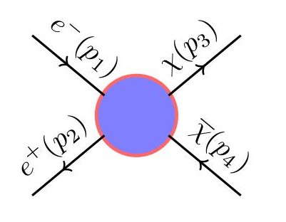
We perform a model-independent analysis for the astrophysical constraints working under the assumption that the DM fermion is leptophilic, i.e. couples directly only to the SM leptons. The specific processes of our interest are (i) (for SN1987A cooling), (ii) (for free-streaming), and (iii) (for relic density), which are all related by crossing symmetry, as shown in Fig. 1. The most general effective Lagrangian leading to these processes is given by the following dimension-six four-Fermi operators [44]:
| (4.1) |
where is the cut-off scale for the EFT description and the index corresponds to different Lorentz structures, such as scalar (S), pseudo-scalar (P), vector (V), axial-vector (A), tensor (T) and axial-tensor (AT) currents. We classify them as follows:
| (4.2) |
where is the spin tensor33 3 We do not write an AT part for , because the ATAT coupling is equivalent to TT, and similarly, TAT is equivalent to ATT due to the identity . and are dimensionless, real couplings. For simplicity, we use a common cut-off scale in Eq. (4.1) for all these operators. Since we are making a model-independent analysis, we do not discuss any specific realization of the above set of effective operators. We investigate SN1987A cooling, DM free-streaming and relic density constraints in light of each of the operator types listed above, taken one at a time, and obtain the corresponding bounds on the cut-off scale as a function of the DM mass. Within the Tsallis statistics framework, we will consider the general case with , as well as the Boltzmann-Gibbs limit of .
4.1 SN1987A Cooling
Electrons are abundant in the supernova core. At high temperatures, positrons are also present, since after ms of the burst, their production is no longer inhibited [80, 90]. These electron-positron pairs can interact via the leptophilic effective operators (4.1) to pair-produce light DM particles: , as shown in Fig. 1.
Once produced, the DM particles can take away a fraction of the energy released in the supernova explosion and contribute to the energy loss rate [16]. Within the framework of Tsallis statistics, the energy loss rate is given by [30]
| (4.3) | |||||
where is the center-of-mass energy ( being the electron and positron energies respectively, which are taken equal here), is the relative velocity between the colliding electron and positron, and is the supernova matter density, are the distribution functions [cf. Eq. (2.8)] and and are the number densities for electron and positron, respectively. The analytic expressions for the cross sections for different four-Fermi operators listed in Eqs. (4.2) are given in Appendix C.1. We will present our numerical results for the simplified case when all the effective coupling parameters in Eq. (4.1) are assumed to be the same and normalized to unity, i.e. (S-P type), (V-A type) and (T-AT type).44 4 This assumption is not valid for a Majorana DM, for which the vectorial and tensorial interactions are forbidden, i.e. . So the bounds derived in Section 5 will have to be reinterpreted accordingly in that scenario. Given the general expressions for the cross sections in Appendix C, our results can be easily translated to other coupling choices. In the simplified case, the expressions (C.1)-(C.3) can be reduced to the following:
| (4.4) | |||||
| (4.5) | |||||
| (4.6) |
where .
Introducing the dimensionless variables (with ), we can write down the energy loss rate in Eq. (4.3) as
| (4.7) |
where . In the supernova core, the electrons and positrons are assumed to be in chemical equilibrium, so . In the limit, the -deformed distribution in Eq. (4.7) approaches the usual Fermi-Dirac distribution, and therefore, the energy loss rate in the undeformed scenario becomes the energy loss rate in the case takes the following form
| (4.8) |
We will use Eqs. (4.7) and (4.8) in our numerical analysis (see Section 5) to compare the energy loss constraints in the -deformed and undeformed scenarios.
4.2 Free-Streaming
As discussed in Section 3.2, the free-streaming of DM from the supernova core depends on the mean free-path of the DM fermion. Given the EFT Lagrangian (4.1), the DM mean free-path is governed by the scattering process and is inversely proportional to the cross-section [cf. Eq. (3.3)]. For different four-Fermi operators listed in Eqs. (4.2), the relevant cross sections are given in Appendix C.2. Under the simplifying assumption that all the effective coupling parameters in Eq. (4.1) are the same and equal to unity, we can rewrite Eqs. (C.4)-(C.6) as
| (4.9) | |||||
| (4.10) | |||||
| (4.11) |
where , where and . We will use the optical depth criterion (3.4) with the mean free path given by Eq. (3.3) and the cross sections given above to derive the free-streaming bounds in Section 5. Note that the mean free-path as such does not depend on the -parameter in the framework of Tsallis statistics. However, as the DM mass exceeds the average supernova core temperature, we should multiply with the effective Boltzmann suppression factor [cf. Eq. (2.8)] to take into account the decreasing DM number density in the core, which induces a mild -dependence, as we will see in Section 5.
4.3 Relic Density
The thermal relic density of DM [cf. Eq. (3.5)] depends on the thermal average of the annihilation cross-section times the relative velocity of the two colliding DM fermions produced in early era. For different four-Fermi operators listed in Eqs. (4.2), the relevant cross sections are given in Appendix C.3. Under the simplifying assumption that all the effective coupling parameters in Eq. (4.1) are the same and equal to unity, the annihilation cross-sections in Eqs. (C.7)-(C.9) can be rewritten as follows:
| (4.12) | |||||
| (4.13) | |||||
| (4.14) |
where and (with being the energies of and , respectively). Also from Eq. (3.7), the thermal averaged cross-section times velocity for the DM fermion pair-annihilation is given by
| (4.15) |
where are the distribution functions for and as given by Eq. (2.8). We will use Eq. (4.15) to calculate the relic density constraints in the following section.
5 Numerical Results
In this section, we use the Tsallis statistics framework [cf. Section 2] and EFT approach [cf. Section 4] to derive the cooling, free-streaming and relic density bounds on the leptophilic DM scenario. For the -deformed distribution function given by Eq. (2.8) and the energy loss rate given by Eq. (4.8), we use the average supernova core temperature of . Similarly, in Eq. (3.4), we use km, in Eq. (4.8), we use the supernova matter density of and chemical potential of , and in Eq. (3.3), we use the electron number density of [16, 91]. For the deformation parameter , we choose a benchmark value of 55 5 This is consistent with the upper bound on from the numerical fits to the supernova neutrino spectrum (see Appendix A). and compare our results with the undeformed scenario with . As for the effective couplings of DM to electrons given by Eqs. (4.2), we assume a simplified case with only one type of interaction at a time and all corresponding couplings being equal and of order unity. The relevant cross section expressions given in Appendix C greatly simplify in this case, as already discussed in the previous Section.
We present our results in the plane of DM mass and the effective cut-off scale . The DM mass is varied between 10 keV–10 GeV. The lower value of the DM mass range is chosen to be consistent with the generic lower bound of keV on fermion DM, based on DM phase space density distribution in dwarf spheroidal galaxies [92, 93]. As for the upper value of the mass range chosen here, this will be justified below, where we show that for , the supernova constraints become weaker than other existing constraints. Our results are shown in Fig. 2 for both undeformed (, left panel) and deformed (, right panel) scenarios. In each case, the solid, dashed and dot-dashed lines correspond to the T-AT type, V-A type and S-P type interactions [cf. Eqs. (4.2)], respectively, taken one at a time and setting the other interactions to zero. Although we show the constraints on the EFT scale all the way down to 10 MeV, one should be careful while applying these constraints to heavier DM. This is because the EFT approach is strictly valid only if the cut-off scale is above the DM mass scale.


5.1 Supernova Cooling Bound
The supernova cooling bounds (red lines) are obtained by using the Raffelt criterion [cf. Section 3.1], i.e. by requiring the energy loss rate given by Eq. (4.8) to be at most the maximum allowed value given by Eq. (3.2). Since the energy loss rate is directly proportional to the cross section and [cf. Eqs. (4.4)-(4.6)], the condition imposes a lower limit on . We find that for a benchmark value of MeV, the undeformed () scenario yields a lower bound on of 2.78, 2.99 and 3.00 TeV for the S-P, V-A and T-AT type operators, respectively, while the deformed scenario with yields a stronger lower bound on of 11.91, 12.80 and 12.81 TeV, respectively. These results are summarized in Table 1. The supernova cooling bounds on are almost independent of the DM mass for , whereas for , the DM production in the supernova core is phase-space suppressed, leading to the exponential weakening of the bound, as is evident from the log-log plot in Fig. 2.
| S-P type | V-A type | T-AT type | ||||
|---|---|---|---|---|---|---|
| SN Cooling | TeV | TeV | TeV | TeV | TeV | TeV |
| Free-streaming | TeV | TeV | TeV | TeV | TeV | TeV |
| Relic Bound | TeV | TeV | TeV | TeV | TeV | TeV |
| XENON10 | TeV | TeV | TeV | |||
| SuperCDMS | TeV | TeV | TeV | |||
| LBECA | TeV | TeV | TeV | |||
| Voyager1 | TeV | TeV | TeV | |||
| Earth Heat Flux | TeV | TeV | TeV | |||
5.2 Free-streaming Bound
The free-streaming bounds (green lines) are obtained from the optical depth criterion [cf. Section 3.2], i.e. by requiring that the mean free path of the DM produced inside the supernova should satisfy the condition given in Eq. (3.4). Since the mean free path is inversely proportional to the cross section [cf. Eq. (3.3)] and [cf. Eqs. (4.9)-(4.11)], the condition (3.4) can be used to derive an upper bound on to be used in conjunction with the lower bound on from supernova cooling. In other words, the values above the green lines and below the red lines are excluded, as shown by the green-shaded regions in Fig. 2. For the values below the green lines, the DM particles do not satisfy the condition (3.4), i.e. they do not free-stream away and are always trapped inside the supernova core, thus invalidating the cooling bound. We find that for a benchmark value of MeV, the undeformed () scenario, we can rule out the values between 0.63-2.78, 1.12-2.99 and 1.21-3.00 TeV for the S-P, V-A and T-AT type operators, respectively, while the deformed scenario with yields a wider exclusion region for between 0.59-11.91, 1.02-12.8 and 1.12-12.81 TeV, respectively [see Table 1]. 66 6 The SN1987A cooling and free-streaming bounds on in this work are found to be a few orders of magnitude smaller than those obtained in earlier works [94, 30] for magnetic and electric dipole moment operators. This follows from the fact that operators used earlier scale as , while in this work, our leptophilic operators given by Eq. (4.1) scale as . Just like in the cooling case, the free-streaming bounds on are almost independent of the DM mass for , whereas for , the DM production and number density in the supernova core is phase-space suppressed, leading to the exponential weakening of the bound, as is evident from the log-log plot in Fig. 2. Note that the mild -dependence of the free-streaming bound comes from the modified distribution function [cf. Eq. (2.8)] for the DM number density.
5.3 Relic Density Bound
The relic density bounds (blue lines) are obtained from Eq. (3.5) which should match the observed DM relic density. Since is directly proportional to the abundance ratio which is inversely proportional to the annihilation cross section [cf.Eq. (3.6)], which in turn goes like [cf. Eqs. (4.12)-(4.14)], the requirement that the DM should not overclose the universe imposes an upper bound on . Note that the observed DM relic density is exactly reproduced only along the blue lines for the corresponding operator type. However, the regions below the blue lines are still allowed in the sense that the missing amount of DM to explain the observed relic density could be obtained by some other means, e.g. by invoking a multi-component, freeze-in or non-thermal DM scenario. In any case, for a thermal relic DM with a benchmark MeV, we find that the undeformed () scenario yields an upper bound on of 0.072, 0.078 and 0.082 TeV for the S-P, V-A and T-AT type operators, respectively, while the deformed scenario with yields a slightly weaker upper bound on of 0.082, 0.088 and 0.091 TeV, respectively [see Table 1]. The bound on increases with the DM mass, because the annihilation cross section , and therefore, to satisfy the observed relic density for a higher DM mass, a correspondingly higher value is needed. The -dependence of the relic density constraint comes from the distribution functions in the thermal averaged annihilation rate [cf. Eq. (3.7)], as well as the effective degrees of freedom in Eq. (3.6). A detailed discussion of the and dependence of is presented in Appendix B.
5.4 Other Experimental Constraints
For comparison, we also translate the direct detection constraints on DM-electron coupling from electron recoil data in XENON10 [10], SuperCDMS [15] and SENSEI [14] onto lower limits on in Fig. 2 (magenta, pink and violet shaded regions, respectively). Specifically, we have used the experimental upper limits on the scattering cross section (for momentum-independent form factor) and compared them with the theoretical predictions given by Eqs. (4.9)-(4.11) with appropriately rescaled . Similar limits can be obtained from XENON100 [12] and DarkSide-50 [13] data, which are not shown here. The XENON10 bound is found to be stronger than the SuperCDMS and SENSEI bounds, but weaker than the astrophysical bounds derived here. However, future limits, such as from LBECA (brown lines) [95] could be comparable to or better than the astrophysical limits in part of the parameter space.
Another lower limit on can be obtained from the constraints due to the heat flux of earth [96], as shown by the cyan shaded region in Fig. 2. For this case also we have used the experimental upper limits on the scattering cross section and compared them with the theoretical predictions given by Eqs. (4.9)-(4.11) with appropriately rescaled . See Table 1 for a quantitative comparison of the direct detection bounds with the astrophysical ones for a benchmark MeV.
We have also converted the indirect detection constraints obtained from cosmic-ray measurements by AMS-02 and Voyager1 [97] onto lower limits on and they are shown in Fig. 2 by the gray and yellow shaded regions, respectively. Here, we have used the experimental upper limits on the thermal average of the annihilation cross section times relative velocity (with ) and compared them with the theoretical predictions given by Eqs. (4.12)-(4.14) and Eq. (4.15). The purple shaded region is excluded from CMB spectral distortion data as measured by FIRAS and the pink curves are the projected CMB limits from PIXIE [98, 99].
There also exist collider constraints on the leptophilic DM scenario. For instance, the effective Lagrangian (4.1) would give rise to the process , which may leave observable signatures in the energy and momentum spectra of the objects (such as photons radiated from the electron or positron leg) recoiling against the DM. The current limits from LEP [101, 100, 102] are found to be much weaker than those shown in Fig. 2, whereas the future limits from ILC [101, 102] could be more competitive.
Similarly, the leptophilic operator (4.1) would also induce an effective DM-quark coupling, but only at the loop-level [44]. Therefore, the hadron collider constraints on monojet/monophoton, as well as the direct detection constraints from nuclear recoil are suppressed, in comparison to the bounds shown in Fig. 2.
5.5 Cooling and Free-streaming at the Crust
As mentioned in Section 3.2, the DM fermions produced in the outer (i.e. crust region) of the supernova free-stream away without any hindrance, whereas the ones produced deep inside are trapped. In this section, we rederive the bounds shown in Fig. 3 for the case when the DM production mechanism is mostly confined to the crust, which has a higher electron density than the core. The average crust temperature is taken to be , mean matter density and mean electron density [16]. Our results are shown in Fig. 3. The only significant change in this case compared to Fig. 2 is for the supernova cooling bounds which become stronger due to the reduced mean matter density and enhanced average temperature at the crust [cf. Eq. (4.8)]. A quantitative comparison of all the limits for a benchmark value of MeV are presented in Table 2.


| S-P type | V-A type | T-AT type | ||||
|---|---|---|---|---|---|---|
| SN Cooling | TeV | TeV | TeV | TeV | TeV | TeV |
| Free-streaming | TeV | TeV | TeV | TeV | TeV | TeV |
| Relic Bound | TeV | TeV | TeV | TeV | TeV | TeV |
| XENON10 | TeV | TeV | TeV | |||
| SuperCDMS | TeV | TeV | TeV | |||
| LBECA | TeV | TeV | TeV | |||
| Voyager1 | TeV | TeV | TeV | |||
| Earth Heat Flux | TeV | TeV | TeV | |||
5.6 Uncertainty on Bound
There is some uncertainty in the mass of the progenitor of SN1987A and the neutrino flux estimation [36, 34, 104]. This amounts to an uncertainty in the knowledge of the core temperature and the matter density of SN1987A. Supernova simulations [105] show the radial variation of the temperature and matter density inside the supernova, which can be encapsulated by the following simple supernova profile [16, 106]:
| (5.1) |
with the core radius, core temperature and core density, respectively. For the fiducial case [106], we have the parameter values and .
Taking into account these different environmental conditions, we have investigated how the bounds on the EFT scale change with respect to the case with constant core temperature and density as discussed above. We find that there is a small change in the free-streaming bound, but the SN cooling bounds can vary up to an order of magnitude. Clearly from accurate supernova modeling, a more precise understanding of the supernova progenitor will improve the robustness of these constraints.
6 Conclusion
We have derived model-independent astrophysical constraints on leptophilic, light, fermionic DM in the framework of Tsallis statistics. In particular, we have considered the DM production in supernova core through its dimension-six, four-Fermi interactions with electrons and positrons, and the subsequent constraints ensuing from supernova cooling due to energy taken away by escaping DM and free-streaming of DM from the outer crust. We find that for an average supernova core temperature of MeV, the SN1987A cooling imposes a lower bound on the effective cut-off scale TeV for the undeformed () case and 12 TeV for the deformed case with for (see Fig. 2 and Table 1). The corresponding limits from the free-streaming and optical depth criteria rule out the values above TeV up to the cooling bound. Restricting the DM production to the outer crust region with a higher MeV yields stronger cooling bounds on TeV (45 TeV) for (see Fig. 3 and Table 2). For , the cooling and free-streaming bounds get significantly weaker due to the Boltzmann-suppression of the DM production and scattering rate in the supernova core. On the other hand, satisfying the observed relic density imposes an upper bound on , which increases with DM mass, and together with the cooling/free-streaming bounds, disfavors a wide parameter range for light leptophilic DM (see Figs. 2 and 3).
Acknowledgments
BD thanks Filippo Sala for an important comment on the free-streaming bound. PKD thanks KC Kong and Doug McKay for several useful discussions. PKD would also like to thank the Department of Physics at Washington University, St. Louis, for arranging a visit while this work was in progress. PKD and BD would like to thank the organizers of WHEPP2018 at IISER, Bhopal, where this work was initiated. The work of BD is supported by the US Department of Energy under Grant No. DE-SC0017987. The work of PKD is partly supported by the SERB Grant No. EMR/2016/002651.
Appendix
Appendix A Upper limit on
Here, we compare the spectrum of the emitted (anti)neutrinos from recent state-of-the-art supernova simulations (see e.g., Ref. [81] for a time-averaged fit and Ref. [82] for a time-dependent fit) with the Tsallis spectrum to derive an upper limit on the value of . Comparing the -deformed distribution function given by Eq. (2.8) for fermions up to the first order with the neutrino distribution function used in Refs. [81, 82]:
| (A.1) |
where is the average neutrino energy, and is the neutrino-spectrum shape parameter (with providing a good fit to the spectrum), we get a relation between and :
| (A.2) |
Given the maximum allowed value of from the fits to the neutrino spectra [81, 82], we obtain from Eq. (A.2) the corresponding value for , which can be considered as the limiting value of the deformation parameter . Hence, the benchmark value of used in our present analysis for the -deformed scenario is consistent with the state-of-the-art supernovae modeling.
Appendix B Effective Degrees of Freedom
To better understand the relic density bound on as a function of and its -dependence, we briefly discuss the temperature and -dependence of the effective degrees of freedom , starting from early times before the electroweak phase transition to the present day. We take the relevant temperature range to be T=(1 keV, 10 TeV), which encapsulates all the essential features we want to study here. From the excellent agreement of the cosmic microwave background with a black body spectrum [2], we know that the early universe was close to thermal equilibrium. Using statistical mechanics, we can calculate the energy density, pressure and entropy density for a system in equilibrium at any given temperature by simply summing up the contributions from all the particle species present in the thermal bath. The contribution from a certain particle species depends on its mass and intrinsic degrees of freedom (such as spin and isospin degeneracy). All this information can be incorporated via the temperature-dependent effective degree of freedom , defined relative to the photon. We have four different functions, i.e., , , and related to the number density, energy density, pressure and entropy density, respectively. By including the intrinsic degrees of freedom () for each particle species , the total effective degrees of freedom for the four kinds mentioned above are given by [107, 108]
| (B.1) | ||||
| (B.2) | ||||
| (B.3) | ||||
| (B.4) |
where , is the Riemann zeta function of argument 3, and the sign is for fermions (bosons). The quantity that appears in Eq. (3.6) for the relic density calculation is only related to the entropy and energy densities [88]:
| (B.5) |
In the -deformed Tsallis statistics formalism, we just replace the normal exponential function in Eqs. (B.1)-(B.4) by the -deformed exponential [cf. Eq. (2.4)] and accordingly the expressions for and get modified. Thus, the temperature-dependent, -deformed effective degree of freedom entering Eq. (3.6) is given by
| (B.6) |
Note that in the limit , we have and we recover the undeformed effective degrees of freedom defined in Eq. (B.5).
In Fig. 4 left panel, we have shown the variation of with in our leptophilic DM setup with a DM mass in order to ensure that the DM has frozen out for the temperature of interest and the only degrees of freedom contributing to are the SM species. We have shown the results for both undeformed () and deformed () cases for comparison. The jumps in the value of are due to different SM species going out-of-equilibrium at that temperature. However, we find that the total effective degrees of freedom is slightly higher in the -deformed case, as compared to the undeformed case, at any given temperature. Similar behavior can be seen in the right panel of Fig. 4, where we plot the variation of with for a fixed temperature (freeze-out temperature), again to ensure that the only degrees of freedom contributing to are the SM species.
The variation of with is shown in Fig. 5 for TeV. As varies from to , steadily increases from to . A change in the value of from 10 to 1 TeV does not lead to any significant change in the value, as shown in Table 3 and Fig. 4). The fact that increases with at a given temperature is a typical feature of the underlying Tsallis statistics and is not to be interpreted as the appearance of any new particle species.
| 10 TeV | |||
|---|---|---|---|
| 1 TeV |
One should note that the QCD phase transition temperature plays an important role in determining the behavior of during the quark-gluon plasma to hot hadron gas transition epoch. In particular, there exists a maximum allowed value, , beyond which we get a very steep, unphysical increase in due to the appearance of many heavier hadrons, whose numbers grow almost exponentially as the temperature increases [107]. The exact value of this maximum phase transition temperature is found to be -dependent in the Tsallis statistics formalism. A variation of against is shown in Fig. 6. As changes from to , is found to vary from MeV to MeV, using which we obtain an empirical formula
| (B.7) |
Note that this is just an upper limit and the actual temperature at which the QCD phase transition occurs is expected to be lower, since there most likely are more possible hadronic states. A more accurate estimate for the transition temperature can be obtained from lattice Monte-Carlo simulations, which suggest MeV [109] in the undeformed scenario, consistent with the upper bound derived here (see Fig. 6).
Appendix C Analytic Expressions for Cross Sections
C.1
| (C.1) | ||||
| (C.2) | ||||
| (C.3) |
where and is the center-of-mass energy.
C.2
| (C.4) | ||||
| (C.5) | ||||
| (C.6) |
C.3
| (C.7) | ||||
| (C.8) | ||||
| (C.9) |
References
- [1] G. Bertone, D. Hooper and J. Silk, Phys. Rept. 405, 279 (2005) [hep-ph/0404175].
- [2] N. Aghanim et al. [Planck Collaboration], arXiv:1807.06209 [astro-ph.CO].
- [3] J. L. Feng, Ann. Rev. Astron. Astrophys. 48, 495 (2010) [arXiv:1003.0904 [astro-ph.CO]].
- [4] E. W. Kolb and M. S. Turner, The early universe, Front. Phys. 69, 1 (1990).
- [5] G. Arcadi, M. Dutra, P. Ghosh, M. Lindner, Y. Mambrini, M. Pierre, S. Profumo and F. S. Queiroz, Eur. Phys. J. C 78, no. 3, 203 (2018) [arXiv:1703.07364 [hep-ph]].
- [6] M. Tanabashi et al. (Particle Data Group), Phys. Rev. D 98, 030001 (2018).
- [7] M. Battaglieri et al., arXiv:1707.04591 [hep-ph].
- [8] R. Essig, J. Mardon and T. Volansky, Phys. Rev. D 85, 076007 (2012) [arXiv:1108.5383 [hep-ph]].
- [9] J. Angle et al. [XENON10 Collaboration], Phys. Rev. Lett. 107, 051301 (2011) Erratum: [Phys. Rev. Lett. 110, 249901 (2013)] [arXiv:1104.3088 [astro-ph.CO]].
- [10] R. Essig, A. Manalaysay, J. Mardon, P. Sorensen and T. Volansky, Phys. Rev. Lett. 109, 021301 (2012) [arXiv:1206.2644 [astro-ph.CO]].
- [11] E. Aprile et al. [XENON100 Collaboration], Science 349, no. 6250, 851 (2015) [arXiv:1507.07747 [astro-ph.CO]].
- [12] E. Aprile et al. [XENON Collaboration], Phys. Rev. D 94, no. 9, 092001 (2016) Erratum: [Phys. Rev. D 95, no. 5, 059901 (2017)] [arXiv:1605.06262 [astro-ph.CO]].
- [13] P. Agnes et al. [DarkSide Collaboration], Phys. Rev. Lett. 121, no. 11, 111303 (2018) [arXiv:1802.06998 [astro-ph.CO]].
- [14] M. Crisler et al. [SENSEI Collaboration], Phys. Rev. Lett. 121, no. 6, 061803 (2018) [arXiv:1804.00088 [hep-ex]].
- [15] R. Agnese et al. [SuperCDMS Collaboration], Phys. Rev. Lett. 121, no. 5, 051301 (2018) [arXiv:1804.10697 [hep-ex]].
- [16] G. G. Raffelt, Stars as laboratories for fundamental physics, University of Chicago Press, Chicago (1996).
- [17] A. Mirizzi, I. Tamborra, H. T. Janka, N. Saviano, K. Scholberg, R. Bollig, L. Hudepohl and S. Chakraborty, Riv. Nuovo Cim. 39, no. 1-2, 1 (2016) [arXiv:1508.00785 [astro-ph.HE]].
- [18] H.-T. Janka, T. Melson and A. Summa, Ann. Rev. Nucl. Part. Sci. 66, 341 (2016) [arXiv:1602.05576 [astro-ph.SR]].
- [19] W. D. Arnett, J. N. Bahcall, R. P. Kirshner and S. E. Woosley, Ann. Rev. Astron. Astrophys. 27, 629 (1989).
- [20] K. Hirata et al. [Kamiokande-II Collaboration], Phys. Rev. Lett. 58, 1490 (1987).
- [21] R. M. Bionta et al., Phys. Rev. Lett. 58, 1494 (1987).
- [22] E. N. Alekseev, L. N. Alekseeva, V. I. Volchenko and I. V. Krivosheina, JETP Lett. 45, 589 (1987).
- [23] E. W. Kolb, R. N. Mohapatra and V. L. Teplitz, Phys. Rev. Lett. 77, 3066 (1996) [hep-ph/9605350].
- [24] P. Fayet, D. Hooper and G. Sigl, Phys. Rev. Lett. 96, 211302 (2006) [hep-ph/0602169].
- [25] J. Hidaka and G. M. Fuller, Phys. Rev. D 74, 125015 (2006) [astro-ph/0609425].
- [26] J. B. Dent, F. Ferrer and L. M. Krauss, arXiv:1201.2683 [astro-ph.CO].
- [27] H. K. Dreiner, J. F. Fortin, C. Hanhart and L. Ubaldi, Phys. Rev. D 89, no. 10, 105015 (2014) [arXiv:1310.3826 [hep-ph]].
- [28] Y. Zhang, JCAP 1411, no. 11, 042 (2014) [arXiv:1404.7172 [hep-ph]].
- [29] D. Kazanas, R. N. Mohapatra, S. Nussinov, V. L. Teplitz and Y. Zhang, Nucl. Phys. B 890, 17 (2014) [arXiv:1410.0221 [hep-ph]].
- [30] A. Guha, Selvaganapathy J. and P. K. Das, Phys. Rev. D 95, no. 1, 015001 (2017) [arXiv:1509.05901 [hep-ph]].
- [31] M. Warren, G. J. Mathews, M. Meixner, J. Hidaka and T. Kajino, Int. J. Mod. Phys. A 31, no. 25, 1650137 (2016) [arXiv:1603.05503 [astro-ph.HE]].
- [32] L. Heurtier and Y. Zhang, JCAP 1702, no. 02, 042 (2017) [arXiv:1609.05882 [hep-ph]].
- [33] H. Tu and K. W. Ng, JHEP 1707, 108 (2017) [arXiv:1706.08340 [hep-ph]].
- [34] C. Mahoney, A. K. Leibovich and A. R. Zentner, Phys. Rev. D 96, no. 4, 043018 (2017) [arXiv:1706.08871 [hep-ph]].
- [35] S. Knapen, T. Lin and K. M. Zurek, Phys. Rev. D 96, no. 11, 115021 (2017) [arXiv:1709.07882 [hep-ph]].
- [36] J. H. Chang, R. Essig and S. D. McDermott, JHEP 1809, 051 (2018) [arXiv:1803.00993 [hep-ph]].
- [37] C. Tsallis, J. Statist. Phys. 52, 479 (1988).
- [38] C. Tsallis, Introduction to Nonextensive Statistical Mechanics : Approaching a Complex World, Springer-Verlag, New York (2001).
- [39] S. Abe and Y. Okamoto (Eds.), Nonextensive Statistical Mechanics and Its Applications, Springer-Verlag, Berlin (2001).
- [40] R. Bernabei et al., Phys. Rev. D 77, 023506 (2008) [arXiv:0712.0562 [astro-ph]].
- [41] M. Cirelli, M. Kadastik, M. Raidal and A. Strumia, Nucl. Phys. B 813, 1 (2009) Addendum: [Nucl. Phys. B 873, 530 (2013)] [arXiv:0809.2409 [hep-ph]].
- [42] C. R. Chen and F. Takahashi, JCAP 0902, 004 (2009) [arXiv:0810.4110 [hep-ph]].
- [43] P. J. Fox and E. Poppitz, Phys. Rev. D 79, 083528 (2009) [arXiv:0811.0399 [hep-ph]].
- [44] J. Kopp, V. Niro, T. Schwetz and J. Zupan, Phys. Rev. D 80, 083502 (2009) [arXiv:0907.3159 [hep-ph]].
- [45] T. Cohen and K. M. Zurek, Phys. Rev. Lett. 104, 101301 (2010) [arXiv:0909.2035 [hep-ph]].
- [46] E. J. Chun, J. C. Park and S. Scopel, JCAP 1002, 015 (2010) [arXiv:0911.5273 [hep-ph]].
- [47] N. Haba, Y. Kajiyama, S. Matsumoto, H. Okada and K. Yoshioka, Phys. Lett. B 695, 476 (2011) [arXiv:1008.4777 [hep-ph]].
- [48] M. Das and S. Mohanty, Phys. Rev. D 89, no. 2, 025004 (2014) [arXiv:1306.4505 [hep-ph]].
- [49] P. S. B. Dev, D. K. Ghosh, N. Okada and I. Saha, Phys. Rev. D 89, 095001 (2014) [arXiv:1307.6204 [hep-ph]].
- [50] P. Agrawal, Z. Chacko and C. B. Verhaaren, JHEP 1408, 147 (2014) [arXiv:1402.7369 [hep-ph]].
- [51] N. F. Bell, Y. Cai, R. K. Leane and A. D. Medina, Phys. Rev. D 90, no. 3, 035027 (2014) [arXiv:1407.3001 [hep-ph]].
- [52] S. M. Boucenna, M. Chianese, G. Mangano, G. Miele, S. Morisi, O. Pisanti and E. Vitagliano, JCAP 1512, no. 12, 055 (2015) [arXiv:1507.01000 [hep-ph]].
- [53] P. S. B. Dev, D. Kazanas, R. N. Mohapatra, V. L. Teplitz and Y. Zhang, JCAP 1608, no. 08, 034 (2016) [arXiv:1606.04517 [hep-ph]].
- [54] B. Q. Lu and H. S. Zong, Phys. Rev. D 93, no. 8, 083504 (2016) Addendum: [Phys. Rev. D 93, no. 8, 089910 (2016)].
- [55] G. H. Duan, L. Feng, F. Wang, L. Wu, J. M. Yang and R. Zheng, JHEP 1802, 107 (2018) [arXiv:1711.11012 [hep-ph]].
- [56] W. Chao, H. K. Guo, H. L. Li and J. Shu, Phys. Lett. B 782, 517 (2018) [arXiv:1712.00037 [hep-ph]].
- [57] Y. Sui and Y. Zhang, Phys. Rev. D 97, no. 9, 095002 (2018) [arXiv:1712.03642 [hep-ph]].
- [58] Z. L. Han, W. Wang and R. Ding, Eur. Phys. J. C 78, no. 3, 216 (2018) [arXiv:1712.05722 [hep-ph]].
- [59] Y. Sui and P. S. B. Dev, JCAP 1807, no. 07, 020 (2018) [arXiv:1804.04919 [hep-ph]].
- [60] C. Y. Chen, J. Kozaczuk and Y. M. Zhong, arXiv:1807.03790 [hep-ph].
- [61] E. Madge and P. Schwaller, arXiv:1809.09110 [hep-ph].
- [62] G. W. Bennett et al. [Muon g-2 Collaboration], Phys. Rev. D 73, 072003 (2006) [hep-ex/0602035].
- [63] R. Bernabei et al., Eur. Phys. J. C 73, 2648 (2013) [arXiv:1308.5109 [astro-ph.GA]].
- [64] R. Bernabei et al., arXiv:1805.10486 [hep-ex].
- [65] J. Chang et al., Nature 456, 362 (2008).
- [66] O. Adriani et al. [PAMELA Collaboration], Nature 458, 607 (2009) [arXiv:0810.4995 [astro-ph]].
- [67] O. Adriani et al. [PAMELA Collaboration], Phys. Rev. Lett. 111, 081102 (2013) [arXiv:1308.0133 [astro-ph.HE]].
- [68] L. Accardo et al. [AMS Collaboration], Phys. Rev. Lett. 113, 121101 (2014).
- [69] M. Aguilar et al. [AMS Collaboration], Phys. Rev. Lett. 113, 121102 (2014).
- [70] S. Abdollahi et al. [Fermi-LAT Collaboration], Phys. Rev. D 95, no. 8, 082007 (2017) [arXiv:1704.07195 [astro-ph.HE]].
- [71] G. Ambrosi et al. [DAMPE Collaboration], Nature 552, 63 (2017) [arXiv:1711.10981 [astro-ph.HE]].
- [72] O. Adriani et al., Phys. Rev. Lett. 120, no. 26, 261102 (2018) [arXiv:1806.09728 [astro-ph.HE]].
- [73] M. Ajello et al. [Fermi-LAT Collaboration], Astrophys. J. 819, no. 1, 44 (2016) [arXiv:1511.02938 [astro-ph.HE]].
- [74] M. G. Aartsen et al. [IceCube Collaboration], arXiv:1710.01191 [astro-ph.HE].
- [75] https://zenodo.org/record/1286919#.W5WwvxgnZhE
- [76] S. Chang, R. Edezhath, J. Hutchinson and M. Luty, Phys. Rev. D 90, no. 1, 015011 (2014) [arXiv:1402.7358 [hep-ph]].
- [77] C. Beck and E. G. D. Cohen, Physica A 322, 267 (2003) [cond-mat/0205097].
- [78] G. Kaniadakis, Phys. Rev. E 66, 056125 (2002).
- [79] C. Beck, Eur. Phys. J. A 40, 267 (2009) [arXiv:0902.2459 [hep-ph]].
- [80] H. T. Janka, K. Langanke, A. Marek, G. Martinez-Pinedo and B. Mueller, Phys. Rept. 442, 38 (2007) [astro-ph/0612072].
- [81] I. Tamborra, B. Muller, L. Hudepohl, H. T. Janka and G. Raffelt, Phys. Rev. D 86, 125031 (2012) [arXiv:1211.3920 [astro-ph.SR]].
- [82] A. Nikrant, R. Laha and S. Horiuchi, Phys. Rev. D 97, no. 2, 023019 (2018) [arXiv:1711.00008 [astro-ph.HE]].
- [83] S. L. Shapiro and S. A. Teukolsky, Black holes, white dwarfs, and neutron stars: the physics of compact objects, A Wiley-interscience publication, Wiley (1983).
- [84] G. G. Raffelt, Astrophys. J. 561, 890 (2001) [astro-ph/0105250].
- [85] H.-T. Janka, Neutrino Emission from Supernovae, In: Alsabti A., Murdin P. (eds) Handbook of Supernovae. Springer, Cham; arXiv:1702.08713 [astro-ph.HE].
- [86] A. Burrows and J. M. Lattimer, Astrophys. J. 307, 178 (1986).
- [87] H. K. Dreiner, C. Hanhart, U. Langenfeld and D. R. Phillips, Phys. Rev. D 68, 055004 (2003) [hep-ph/0304289].
- [88] P. Gondolo and G. Gelmini, Nucl. Phys. B 360, 145 (1991).
- [89] A. Guha and P. K. Das, JHEP 1806, 139 (2018) [arXiv:1803.04540 [hep-ph]].
- [90] H. A. Bethe, Rev. Mod. Phys. 62, 801 (1990).
- [91] A. Burrows, M. S. Turner and R. P. Brinkmann, Phys. Rev. D 39, 1020 (1989).
- [92] S. Tremaine and J. E. Gunn, Phys. Rev. Lett. 42, 407 (1979).
- [93] A. Boyarsky, O. Ruchayskiy and D. Iakubovskyi, JCAP 0903, 005 (2009) [arXiv:0808.3902 [hep-ph]].
- [94] K. Kadota and J. Silk, Phys. Rev. D 89, no. 10, 103528 (2014) [arXiv:1402.7295 [hep-ph]].
- [95] R. Lang, News from Dark Matter Direct Searches, Talk at PHENO2018, https://indico.cern.ch/event/699148/
- [96] B. Chauhan and S. Mohanty, Phys. Rev. D 94, no. 3, 035024 (2016) [arXiv:1603.06350 [hep-ph]].
- [97] M. Boudaud, J. Lavalle and P. Salati, Phys. Rev. Lett. 119, no. 2, 021103 (2017) [arXiv:1612.07698 [astro-ph.HE]].
- [98] Y. Ali-Haïmoud, J. Chluba and M. Kamionkowski, Phys. Rev. Lett. 115, no. 7, 071304 (2015) [arXiv:1506.04745 [astro-ph.CO]].
- [99] C. V. Cappiello, K. C. Y. Ng and J. F. Beacom, arXiv:1810.07705 [hep-ph].
- [100] P. J. Fox, R. Harnik, J. Kopp and Y. Tsai, Phys. Rev. D 84, 014028 (2011) [arXiv:1103.0240 [hep-ph]].
- [101] Y. J. Chae and M. Perelstein, JHEP 1305, 138 (2013) [arXiv:1211.4008 [hep-ph]].
- [102] A. Freitas and S. Westhoff, JHEP 1410, 116 (2014) [arXiv:1408.1959 [hep-ph]].
- [103] S. Horiuchi and J. P. Kneller, J. Phys. G 45, no. 4, 043002 (2018) [arXiv:1709.01515 [astro-ph.HE]].
- [104] M. T. Keil, G. G. Raffelt and H. T. Janka, Astrophys. J. 590, 971 (2003) [astro-ph/0208035].
- [105] P. Char, S. Banik and D. Bandyopadhyay, Astrophys. J. 809, no. 2, 116 (2015) [arXiv:1508.01854 [astro-ph.HE]].
- [106] J. H. Chang, R. Essig and S. D. McDermott, JHEP 1701, 107 (2017) [arXiv:1611.03864 [hep-ph]].
- [107] L. Husdal, Galaxies 4, no. 4, 78 (2016) [arXiv:1609.04979 [astro-ph.CO]].
- [108] B. Ryden, Introduction to Cosmology, Addison-Wesley, San Francisco (2003).
- [109] P. Petreczky, J. Phys. G 39, 093002 (2012) [arXiv:1203.5320 [hep-lat]].