跳到论文正文
W Papers独立论文阅读器 arXiv:1810.00212 论文正文 计算阅读时间 · 0%
引用这篇论文根据当前论文元数据生成,正式投稿前建议核对。


License: arXiv.org perpetual non-exclusive license
arXiv:1810.00212v3 [math.GT] 27 Aug 2019

On hyperbolic surface bundles over the circle as branched double covers of the 33-sphere

Susumu Hirose Address: Department of Mathematics, Faculty of Science and Technology, Tokyo University of Science, Noda, Chiba, 278-8510, Japan Email address: hirose_susumu@ma.noda.tus.ac.jp and Eiko Kin Address: Department of Mathematics, Graduate School of Science, Osaka University Toyonaka, Osaka 560-0043, JAPAN Email address: kin@math.sci.osaka-u.ac.jp
Date: August 8, 2019
Abstract.

The branched virtual fibering theorem by Sakuma states that every closed orientable 33-manifold with a Heegaard surface of genus gg has a branched double cover which is a genus gg surface bundle over the circle. It is proved by Brooks that such a surface bundle can be chosen to be hyperbolic. We prove that the minimal entropy over all hyperbolic, genus gg surface bundles as branched double covers of the 33-sphere behaves like 1/gg. We also give an alternative construction of surface bundles over the circle in Sakuma’s theorem when closed 33-manifolds are branched double covers of the 33-sphere branched over links. A feature of surface bundles coming from our construction is that the monodromies can be read off the braids obtained from the links as the branched set.

Key words and phrases: 
pseudo-Anosov, dilatation (stretch factor), 22-fold branched cover of the 33-sphere, fibered 33-manifold, Heegaard surface, mapping class groups, braid groups
2000 Mathematics Subject Classification
Primary 57M27, 37E30, Secondary 37B40

1. Introduction

This paper concerns the branched virtual fibering theorem by Makoto Sakuma. To state his theorem let Σ=Σg,p\Sigma=\Sigma_{g,p} be an orientable, connected surface of genus gg with pp punctures possibly p=0p=0, and let us set Σg=Σg,0\Sigma_{g}=\Sigma_{g,0}. The mapping class group Mod⁡(Σ)\mathrm{Mod}(\Sigma) is the group of isotopy classes of orientation-preserving self-homeomorphisms on Σ\Sigma which preserve the punctures setwise. By Nielsen-Thurston classification, elements in Mod⁡(Σ)\mathrm{Mod}(\Sigma) fall into three types: periodic, reducible, pseudo-Anosov [9]. To each pseudo-Anosov element ϕ\phi, there is an associated dilatation (stretch factor) λ⁡(ϕ)>1\lambda(\phi)>1 (see [4] for example). We call the logarithm of the dilatation log⁡(λ⁡(ϕ))\log(\lambda(\phi)) the entropy of ϕ\phi.

Choosing a representative f:Σ→Σf:\Sigma\to\Sigma of ϕ\phi we define the mapping torus TϕT_{\phi} by

Tϕ=Σ×ℝ/∼,T_{\phi}=\Sigma\times\mathbb{R}/\sim,

where (x,t)∼(f⁡(x),t+1)(x,t)\sim(f(x),t+1) for x∈Σx\in\Sigma, t∈ℝt\in\mathbb{R}. We call Σ\Sigma the fiber surface of TϕT_{\phi}. The 33-manifold TϕT_{\phi} is a Σ\Sigma-bundle over the circle with the monodromy ϕ\phi. By Thurston [10] TϕT_{\phi} admits a hyperbolic structure of finite volume if and only if ϕ\phi is pseudo-Anosov.

The following theorem is due to Sakuma [8, Addendum 1]. See also [3, Section 3].

Theorem 1 (Branched virtual fibering theorem).

Let MM be a closed orientable 33-manifold. Suppose that MM admits a genus gg Heegaard splitting. Then there is a 22-fold branched cover M~\widetilde{M} of MM which is a Σg\Sigma_{g}-bundle over the circle.

It is proved by Brooks [3] that M~\widetilde{M} in Theorem 1 can be chosen to be hyperbolic if g≥max⁡(2,g⁡(M))g\geq\max(2,g(M)), where g⁡(M)g(M) is the Heegaard genus of MM. See also [6] by Montesinos.

Let Dg​(M)D_{g}(M) be the subset of Mod⁡(Σg)\mathrm{Mod}(\Sigma_{g}) consisting of elements ϕ\phi such that TϕT_{\phi} is homeomorphic to a 22-fold branched cover of MM branched over some link. By Theorem 1 we have Dg​(M)≠∅D_{g}(M)\neq\emptyset. By Brooks together with the stabilization of Heegaard splittings, there is a pseudo-Anosov element in Dg​(M)D_{g}(M) for each g≥max⁡(2,g⁡(M))g\geq\max(2,g(M)). The set of fibered 33-manifolds TϕT_{\phi} over all ϕ∈Dg​(M)\phi\in D_{g}(M) possesses various properties inherited under branched covers of MM. It is natural to ask about the dynamics of pseudo-Anosov elements in Dg​(M)D_{g}(M). We are interested in the set of entropies of pseudo-Anosov mapping classes.

We fix a surface Σ\Sigma and consider the set of entropies

{log⁡λ⁡(ϕ)|ϕ∈Mod⁡(Σ)​is pseudo-Anosov}\{\log\lambda(\phi)\ |\ \phi\in\mathrm{Mod}(\Sigma)\ \mbox{is pseudo-Anosov}\}

which is a closed, discrete subset of ℝ{\mathbb{R}} ([1]). For any subset G⊂Mod⁡(Σ)G\subset\mathrm{Mod}(\Sigma) let δ⁡(G)\delta(G) denote the minimum of dilatations λ⁡(ϕ)\lambda(\phi) over all pseudo-Anosov elements ϕ∈G\phi\in G. Then δ⁡(G)≥δ⁡(Mod⁡(Σ))\delta(G)\geq\delta(\mathrm{Mod}(\Sigma)). For real valued functions ff and hh, we write f≍hf\asymp h if there is a universal constant cc such that h/c≤f≤c​hh/c\leq f\leq ch. It is proved by Penner [7] that

log⁡δ⁡(Mod⁡(Σg))≍1g.\log\delta(\mathrm{Mod}(\Sigma_{g}))\asymp\dfrac{1}{g}.

A question arises: what can we say about the asymptotic behavior of the minimal entropies log⁡δ​(Dg​(M))\log\delta(D_{g}(M))’s for each closed 33-manifold MM? In this paper we consider this question when MM is the 33-sphere S3S^{3}. Our main theorem is the following.

Theorem A.

We have log⁡δ⁡(Dg​(S3))≍1g\log\delta(D_{g}(S^{3}))\asymp\dfrac{1}{g}.

Refer to caption
Figure 1. (1) σi∈Bn\sigma_{i}\in B_{n}. (2) Involution on the cylinder. Thick segment in the middle is the fixed point set of the involution. (3) b~=skew⁡(b)⋅b\widetilde{b}=\operatorname{skew}(b)\cdot b is invariant under such an involution.

Let qL:ML→S3q_{L}:M_{L}\rightarrow S^{3} denote the 22-fold branched covering map of S3S^{3} branched over a link LL in S3S^{3}. Along the way in the proof of Theorem A we give an alternative proof of Theorem 1 when M=MLM=M_{L} in Theorem B. A feature of surface bundles ML~\widetilde{M_{L}} coming from our construction is that their monodromies can be read off the braids obtained from the links as the branched set. To state Theorem B, we need 3 ingredients.

1. Involution skew:Bn→Bn\operatorname{skew}:B_{n}\to B_{n}. Let BnB_{n} be the (planar) braid group with nn strands and let σi\sigma_{i} denote the Artin generator of BnB_{n} as in Figure 1(1). We define an involution

skew:Bn\displaystyle\operatorname{skew}:B_{n} →\displaystyle\to Bn\displaystyle B_{n}
σn1ϵ1σn2ϵ2⋯σnkϵk\displaystyle\sigma_{n_{1}}^{\epsilon_{1}}\sigma_{n_{2}}^{\epsilon_{2}}\cdots\sigma_{n_{k}}^{\epsilon_{k}} ↦\displaystyle\mapsto σn−nkϵk⋯σn−n2ϵ2σn−n1ϵ1,ϵi=±1.\displaystyle\sigma_{n-n_{k}}^{\epsilon_{k}}\cdots\sigma_{n-n_{2}}^{\epsilon_{2}}\sigma_{n-n_{1}}^{\epsilon_{1}},\hskip 14.22636pt\epsilon_{i}=\pm 1.

We say that b∈Bnb\in B_{n} is skew-palindromic if skew⁡(b)=b\operatorname{skew}(b)=b. The braid skew⁡(b)⋅b\operatorname{skew}(b)\cdot b is skew-palindromic for any b∈Bnb\in B_{n}. (There is a skew-palindromic braid which can not be written by skew⁡(b)⋅b\operatorname{skew}(b)\cdot b for any bb, for example σ1​σ2​σ3∈B4\sigma_{1}\sigma_{2}\sigma_{3}\in B_{4}.) We write

b~=skew⁡(b)⋅b.\widetilde{b}=\operatorname{skew}(b)\cdot b.

Note that skew:Bn→Bn\operatorname{skew}:B_{n}\rightarrow B_{n} is induced by the involution on the cylinder as shown in Figure 1(2) and skew-palindromic braids are invariant under such an involution.

In the later section, the map skew\operatorname{skew} is also regarded as a map from the braid group on the sphere or the annulus to itself. The above assertion for the braid b~=skew⁡(b)⋅b\widetilde{b}=\operatorname{skew}(b)\cdot b also holds in this setting.

Refer to caption
Figure 2. Simple closed curves on Σg\Sigma_{g}.

2. Homomorphism 𝔱:B2​g+2→Mod⁡(Σg)\mathfrak{t}:B_{2g+2}\rightarrow\mathrm{Mod}(\Sigma_{g}). Let tit_{i} denote the right-handed Dehn twist about the simple closed curve with the number ii in Figure 2. Then there is a homomorphism

𝔱:B2​g+2→Mod⁡(Σg)\mathfrak{t}:B_{2g+2}\rightarrow\mathrm{Mod}(\Sigma_{g})

which sends σi\sigma_{i} to tit_{i} for i=1,…,2​g+1i=1,\ldots,2g+1, since Mod⁡(Σg)\mathrm{Mod}(\Sigma_{g}) has the braid relation. (We apply elements of mapping class groups from right to left.) The hyperelliptic mapping class group ℋ⁡(Σg)\mathcal{H}(\Sigma_{g}) is the subgroup of Mod⁡(Σg)\mathrm{Mod}(\Sigma_{g}) consisting of elements with representative homeomorphisms that commute with some fixed hyperelliptic involution. By Birman-Hilden [2], ℋ⁡(Σg)\mathcal{H}(\Sigma_{g}) is generated by tit_{i}’s. Thus

ℋ⁡(Σg)=𝔱⁡(B2​g+2).\mathcal{H}(\Sigma_{g})=\mathfrak{t}(B_{2g+2}).

3. Circular plat closure C⁡(b)C(b). We use two types of links in S3S^{3} obtained from braids. One is the closure cl⁡(β)\mathrm{cl}(\beta) of β\beta ∈Bg+1\in B_{g+1} as in Figure 3(1). The other is the circular plat closure C⁡(b)C(b) of b∈B2​g+2b\in B_{2g+2} with even strands as in Figure 3(2)(3). We also use the link C⁡(b)∪WC(b)\cup W, the union of C⁡(b)C(b) and the trivial link W=O∪O′W=O\cup O^{\prime} with 22 components as shown in Figure 3(4).

Refer to caption
Figure 3. (1) cl⁡(β)\mathrm{cl}(\beta) for β∈Bg+1\beta\in B_{g+1} and β′∈B2​g+2\beta^{\prime}\in B_{2g+2}. (2) C⁡(b)C(b) for b∈B2​g+2b\in B_{2g+2}. (3) C⁡(σ3​σ4​σ5)C(\sigma_{3}\sigma_{4}\sigma_{5}). (4) C⁡(b)∪WC(b)\cup W, where W=O∪O′W=O\cup O^{\prime}.

Any link in S3S^{3} can be represented by C⁡(β′)C(\beta^{\prime}) for some braid β′\beta^{\prime}. To see this, it is well-known that LL is the closure cl⁡(β)\mathrm{cl}(\beta) for some β∈Bg+1\beta\in B_{g+1} (g≥1g\geq 1). The desired braid β′∈B2​g+2\beta^{\prime}\in B_{2g+2} can be obtained from β\beta by adding g+1g+1 straight strands as in Figure 3(1).

For a braid b∈B2​g+2b\in B_{2g+2} let q=qC⁡(b):MC⁡(b)→S3q=q_{C(b)}:M_{C(b)}\rightarrow S^{3} be the 22-fold branched covering map of S3S^{3} branched over C⁡(b)C(b). There is a (g+1)(g+1)-bridge sphere SS for the link C⁡(b)⊂S3C(b)\subset S^{3}. Hence MC⁡(b)M_{C(b)} admits a genus gg Heegaard splitting with the Heegaard surface q−1​(S)q^{-1}(S). Then we have the following result.

Theorem B.

Let MC⁡(b)~\widetilde{M_{C(b)}} be the 22-fold branched cover of MC⁡(b)M_{C(b)} branched over the link q−1​(W)q^{-1}(W). Then MC⁡(b)~\widetilde{M_{C(b)}} is homeomorphic to the mapping torus T𝔱⁡(b~)T_{\mathfrak{t}(\widetilde{b})}.

Remark 2.

To be precise, MC⁡(b)~\widetilde{M_{C(b)}} is the 22-fold branched cover of MC⁡(b)M_{C(b)} branched over q−1​(W)q^{-1}(W) obtained as the ℤ/2​ℤ+ℤ/2​ℤ{\mathbb{Z}}/2{\mathbb{Z}}+{\mathbb{Z}}/2{\mathbb{Z}}-cover of S3S^{3} branched over the link C⁡(b)∪WC(b)\cup W associated with the epimorphism H1​(S3∖(C⁡(b)∪W))→ℤ/2​ℤ+ℤ/2​ℤH_{1}(S^{3}\setminus(C(b)\cup W))\rightarrow{\mathbb{Z}}/2{\mathbb{Z}}+{\mathbb{Z}}/2{\mathbb{Z}} which maps the meridians of C⁡(b)C(b) to the generator of the first factor and the meridians of WW to the generator of the second factor.

Acknowledgments. We thank Makoto Sakuma and Yuya Koda for helpful conversations and comments. We also thank the anonymous referee for valuable comments. The first author was supported by Grant-in-Aid for Scientific Research (C) (No. 16K05156), JSPS. The second author was supported by Grant-in-Aid for Scientific Research (C) (No. 18K03299), JSPS.

2. Proof of Theorem B

Proof of Theorem B.

We construct the 33-sphere S3S^{3} from two copies of the 33-ball B3B^{3} by gluing their boundaries together. Consider the link C⁡(b)∪WC(b)\cup W so that C⁡(b)C(b) is contained in one of the 33-balls, and WW is given by the union of the four thick segments in the two 33-balls, see Figure 4(2). Let SS be the sphere in S3S^{3} which is the union of the two shaded disks in the same figure. The 22-sphere SS is a (g+1)(g+1)-bridge sphere for C⁡(b)C(b), and the preimage q−1​(S)q^{-1}(S) is a genus gg Heegaard surface of MC⁡(b)M_{C(b)}.

Let qW:MW→S3q_{W}:M_{W}\to S^{3} be the 22-fold branched covering map of S3S^{3} branched over WW (Figure 4(1)). The preimage qW−1​(B3)q^{-1}_{W}(B^{3}) is homeomorphic to the solid torus D2×S1D^{2}\times S^{1}. Then MWM_{W} is obtained from two copies of D2×S1D^{2}\times S^{1} by gluing their boundaries together, and hence MWM_{W} is homeomorphic to S2×S1S^{2}\times S^{1}. Observe that the link qW−1​(C​(b))q_{W}^{-1}(C(b)) is the closure of the spherical braid b~=skew⁡(b)⋅b\widetilde{b}=\operatorname{skew}(b)\cdot b, i.e.,

qW−1​(C⁡(b))=cl⁡(b~)⊂S2×S1.q_{W}^{-1}(C(b))=\mathrm{cl}(\widetilde{b})\subset S^{2}\times S^{1}.

Let p:Ncl⁡(b~)→S2×S1p:N_{\mathrm{cl}(\widetilde{b})}\rightarrow S^{2}\times S^{1} be the 22-fold branched covering map of S2×S1S^{2}\times S^{1} branched over cl⁡(b~)\mathrm{cl}(\widetilde{b}). The 22-fold branched cover of the level surface S2×{u}S^{2}\times\{u\} for u∈S1u\in S^{1} branched at the 2​g+22g+2 points in ((S2×{u})∩cl⁡(b~))\Bigl((S^{2}\times\{u\})\cap\mathrm{cl}(\widetilde{b})\Bigr) is a closed surface of genus gg. Thus Ncl⁡(b~)N_{\mathrm{cl}(\widetilde{b})} is a Σg\Sigma_{g}-bundle over S1S^{1} with the monodromy 𝔱⁡(b~)\mathfrak{t}(\widetilde{b}), i.e., Ncl⁡(b~)N_{\mathrm{cl}(\widetilde{b})} is homeomorphic to T𝔱⁡(b~)T_{\mathfrak{t}(\widetilde{b})}.

We can observe that the composition

qW∘p:T𝔱⁡(b~)≅Ncl⁡(b~)→S3q_{W}\circ p:T_{\mathfrak{t}(\widetilde{b})}\cong N_{\mathrm{cl}(\widetilde{b})}\rightarrow S^{3}

is the ℤ/2​ℤ+ℤ/2​ℤ{\mathbb{Z}}/2{\mathbb{Z}}+{\mathbb{Z}}/2{\mathbb{Z}}-cover of S3S^{3} branched over the link C⁡(b)∪WC(b)\cup W described in Remark 2. Hence T𝔱⁡(b~)≅Ncl⁡(b~)T_{\mathfrak{t}(\widetilde{b})}\cong N_{\mathrm{cl}(\widetilde{b})} is identified with 22-fold branched cover MC⁡(b)~\widetilde{M_{C(b)}}. This completes the proof. ∎

Refer to caption
Figure 4. (1) cl⁡(b~)⊂S2×S1\mathrm{cl}(\widetilde{b})\subset S^{2}\times S^{1}. (2) C⁡(b)∪W⊂S3C(b)\cup W\subset S^{3}. (3) Diagram: MC⁡(b)~→MC⁡(b)\widetilde{M_{C(b)}}\rightarrow M_{C(b)} is the 22-fold branched cover of MC⁡(b)M_{C(b)} branched over q−1​(W)q^{-1}(W).

3. Proof of Theorem A

Refer to caption
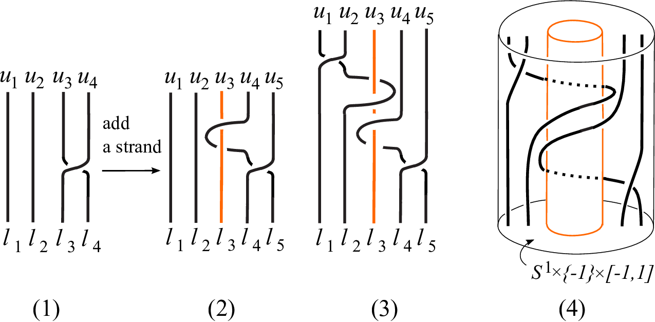
Figure 5. (1) b=σ3b=\sigma_{3}. (2) b∘=σ32​σ4b^{\circ}=\sigma_{3}^{2}\sigma_{4}. (3) b∘~\widetilde{b^{\circ}}. (b~=σ1​σ3\widetilde{b}=\sigma_{1}\sigma_{3} is obtained from b∘~\widetilde{b^{\circ}} by removing the strand with endpoints ℓ3\ell_{3} and u3u_{3}.) (4) Braid b~\widetilde{b} on 𝒜\mathcal{A}.

Given a braid bb we first give a construction of a braid b′b^{\prime} (with more strands than bb) such that C⁡(b)C(b) is ambient isotopic to C⁡(b′)C(b^{\prime}).

The bottom and top endpoints of a planar braid with nn strands are denoted by l1,…,lnl_{1},\ldots,l_{n} and u1,…,unu_{1},\ldots,u_{n} from left to right. For a braid b∈B2​g+2b\in B_{2g+2} with even strands, we choose a braid b∘∈B2​g+3b^{\circ}\in B_{2g+3} obtained from bb by adding a strand, say b∘​(g+2)b^{\circ}(g+2) connecting the middle of the two points lg+1l_{g+1} and lg+2l_{g+2} with the middle of the two points ug+1u_{g+1} and ug+2u_{g+2}. Of course b∘b^{\circ} is not unique. For example when b=b1=σ3∈B4b=b_{1}=\sigma_{3}\in B_{4}, one can choose b∘(=b1∘)=σ32​σ4∈B5b^{\circ}(=b_{1}^{\circ})=\sigma_{3}^{2}\sigma_{4}\in B_{5}. See Figure 5.

We consider b∘~=skew⁡(b∘)⋅b∘∈B2​g+3\widetilde{b^{\circ}}=\operatorname{skew}(b^{\circ})\cdot b^{\circ}\in B_{2g+3} with bottom endpoints l1,…,l2​g+3l_{1},\ldots,l_{2g+3} and top endpoints u1,…,u2​g+3u_{1},\ldots,u_{2g+3}. The braid b∘~\widetilde{b^{\circ}} has the strand b∘~​(g+2)\widetilde{b^{\circ}}(g+2) with endpoints lg+2l_{g+2} and ug+2u_{g+2}. If we remove this strand from b∘~\widetilde{b^{\circ}}, then we obtain b~=skew⁡(b)⋅b\widetilde{b}=\operatorname{skew}(b)\cdot b.

Refer to caption
Figure 6. (1) Solid torus (D2×S1)−1(D^{2}\times S^{1})_{-1}. (2) S1×S1×[−1,1]S^{1}\times S^{1}\times[-1,1] obtained from S1×[−1,1]×[−1,1]S^{1}\times[-1,1]\times[-1,1] by identifying the two annuli S1×{1}×[−1,1]S^{1}\times\{1\}\times[-1,1] and S1×{−1}×[−1,1]S^{1}\times\{-1\}\times[-1,1]. (3) Solid torus (D2×S1)+1(D^{2}\times S^{1})_{+1}.

Now we construct S2×S1S^{2}\times S^{1} from three pieces, two solid tori (D2×S1)±1(D^{2}\times S^{1})_{\pm 1} and the product S1×S1×[−1,1]S^{1}\times S^{1}\times[-1,1] of a torus S1×S1S^{1}\times S^{1} and the interval [−1,1][-1,1] by gluing (∂D2×S1)i(\partial D^{2}\times S^{1})_{i} to S1×S1×{i}S^{1}\times S^{1}\times\{i\} together for i=±1i=\pm 1. See Figure 6. We think of S1S^{1} as the quotient space [−1,1]/(−1∼1)[-1,1]/(-1\sim 1), and consider the product

S1×S1×[−1,1]=S1×[−1,1]/(−1∼1)×[−1,1].S^{1}\times S^{1}\times[-1,1]=S^{1}\times[-1,1]/(-1\sim 1)\times[-1,1].

For the braided link br⁡(b∘~)=cl⁡(b∘~)∪A\mathrm{br}(\widetilde{b^{\circ}})=\mathrm{cl}(\widetilde{b^{\circ}})\cup A in S3S^{3}, we perform the 00-surgery along the braid axis AA. Then the image of cl⁡(b∘~)\mathrm{cl}(\widetilde{b^{\circ}}) forms a link in S2×S1S^{2}\times S^{1}, which continues to denote by the same symbol cl⁡(b∘~)\mathrm{cl}(\widetilde{b^{\circ}}). We deform this link cl⁡(b∘~)\mathrm{cl}(\widetilde{b^{\circ}}) in S2×S1S^{2}\times S^{1} so that the knot cl​(b∘~​(g+2))\mathrm{cl}(\widetilde{b^{\circ}}(g+2)) becomes the core of (D2×S1)−1(D^{2}\times S^{1})_{-1} and cl⁡(b~)=cl⁡(b∘~)∖cl⁡(b∘~​(g+2))\mathrm{cl}(\widetilde{b})=\mathrm{cl}(\widetilde{b^{\circ}})\setminus\mathrm{cl}(\widetilde{b^{\circ}}(g+2)) is contained in S1×S1×[−1,1]S^{1}\times S^{1}\times[-1,1]. One can regard b~\widetilde{b} as a braid on the annulus 𝒜:=S1×{−1}×[−1,1]\mathcal{A}:=S^{1}\times\{-1\}\times[-1,1] which is embedded in S1×[−1,1]×[−1,1]S^{1}\times[-1,1]\times[-1,1], and one can think of the link cl⁡(b~)\mathrm{cl}(\widetilde{b}) as the closure of the braid b~\widetilde{b} on 𝒜\mathcal{A}. See Figure 5(4). Let

R:S2×S1→S2×S1R:S^{2}\times S^{1}\rightarrow S^{2}\times S^{1}

be the deck transformation of qW:S2×S1→S3q_{W}:S^{2}\times S^{1}\to S^{3} in the proof of Theorem B. Then qWq_{W} sends the fixed point set of the involution RR to the trivial link WW (Figure 4(1)(2)). Let

f:S1×S1→S1×S1f:S^{1}\times S^{1}\rightarrow S^{1}\times S^{1}

be any orientation-preserving homeomorphism. We may assume that ff commutes with the involution

ι:S1×S1\displaystyle\iota:S^{1}\times S^{1} →\displaystyle\to S1×S1\displaystyle S^{1}\times S^{1}
(x,y)\displaystyle(x,y) ↦\displaystyle\mapsto (−x,−y).\displaystyle(-x,-y).

We consider the homeomorphism

Φf=f×id[−1,1]:S1×S1×[−1,1]→S1×S1×[−1,1].\Phi_{f}=f\times\mathrm{id}_{[-1,1]}:S^{1}\times S^{1}\times[-1,1]\rightarrow S^{1}\times S^{1}\times[-1,1].

The image of cl⁡(b~)\mathrm{cl}(\widetilde{b}) under Φf\Phi_{f} may or may not be the closure of some braid on 𝒜\mathcal{A}. We assume the former case (∗)(*):

(∗)(*) Φf​(cl⁡(b~))=cl⁡(γ)\Phi_{f}(\mathrm{cl}(\widetilde{b}))=\mathrm{cl}(\gamma) for some braid γ\gamma on 𝒜\mathcal{A}.

Then the involution R|S1×S1×[−1,1]=ι×id[−1,1]R|_{S^{1}\times S^{1}\times[-1,1]}=\iota\times\mathrm{id}_{[-1,1]} has the following property.

R⁡(cl⁡(β))=cl⁡(skew⁡(β))​for any braid ​β​ on​𝒜.R(\mathrm{cl}(\beta))=\mathrm{cl}(\operatorname{skew}(\beta))\hskip 5.69054pt\mbox{for any braid }\beta\mbox{ on}\ \mathcal{A}.

cf. Figure 1(2). Since ff commutes with ι\iota, it follows that Φf\Phi_{f} commutes with R|S1×S1×[−1,1]R|_{S^{1}\times S^{1}\times[-1,1]}. Hence we have

cl⁡(γ)=Φf​(cl⁡(b~))=Φf​(cl⁡(skew⁡(b~)))=Φf​R​(cl⁡(b~))=R​Φf​(cl⁡(b~))=R⁡(cl⁡(γ)).\mathrm{cl}(\gamma)=\Phi_{f}(\mathrm{cl}(\widetilde{b}))=\Phi_{f}(\mathrm{cl}(\operatorname{skew}(\widetilde{b})))=\Phi_{f}R(\mathrm{cl}(\widetilde{b}))=R\Phi_{f}(\mathrm{cl}(\widetilde{b}))=R(\mathrm{cl}(\gamma)).

(The first and last equality come from the assumption (∗)(*), and the second equality holds since b~\widetilde{b} is skew-palindromic.) Thus cl⁡(γ)=R⁡(cl⁡(γ))\mathrm{cl}(\gamma)=R(\mathrm{cl}(\gamma)). We further assume that

(∗∗)(**) (Φf​(cl⁡(b~))=)​cl​(γ)=cl⁡(bf~)\bigl(\Phi_{f}(\mathrm{cl}(\widetilde{b}))=\bigr)\mathrm{cl}(\gamma)=\mathrm{cl}(\widetilde{b_{f}}) for some braid bfb_{f} on 𝒜\mathcal{A}.

Remark 3.

Clearly (∗∗)(**) implies cl⁡(γ)=R⁡(cl⁡(γ))\mathrm{cl}(\gamma)=R(\mathrm{cl}(\gamma)). It is likely the converse holds.

Now, we think of the braid bfb_{f} on 𝒜\mathcal{A} as a planar braid as in Figure 5, and consider the link C⁡(bf)C(b_{f}) in S3S^{3}. We have the following lemma.

Lemma 4.

Under the assumptions (∗)(*) and (∗∗)(**), C⁡(b)C(b) and C⁡(bf)C(b_{f}) are ambient isotopic.

Proof.

Note that the quotient (S1×S1×[−1,1])/R\big(S^{1}\times S^{1}\times[-1,1]\big)/R is homeomorphic to S2×[−1,1]S^{2}\times[-1,1]. Since Φf\Phi_{f} commutes with R|S1×S1×[−1,1]R|_{S^{1}\times S^{1}\times[-1,1]}, Φf\Phi_{f} induces a self-homeomorphism

Φ¯f:S2×[−1,1]→S2×[−1,1].\underline{\Phi}_{f}:S^{2}\times[-1,1]\rightarrow S^{2}\times[-1,1].

Since Φf​(cl⁡(b~))=cl⁡(bf~)\Phi_{f}(\mathrm{cl}(\widetilde{b}))=\mathrm{cl}(\widetilde{b_{f}}) we have Φ¯f​(C⁡(b))=C⁡(bf)\underline{\Phi}_{f}(C(b))=C(b_{f}). Any orientation-preserving self-homeomorphism on S2S^{2} is isotopic to the identity, and S3S^{3} is a union of S2×[−1,1]S^{2}\times[-1,1] and two 33-balls by gluing the boundaries together. Thus Φ¯f\underline{\Phi}_{f} extends to a self-homeomorphism on S3S^{3} which sends C⁡(b)C(b) to C⁡(bf)C(b_{f}). This completes the proof. ∎

Refer to caption
Figure 7. (1) Shaded region indicates annulus 𝔸{\mathbb{A}} with boundary {v}×S1×{±1}\{v\}\times S^{1}\times\{\pm 1\}. (3) cl⁡(b1~)\mathrm{cl}(\widetilde{b_{1}}) and (4) Φf​(cl⁡(b1~))=cl⁡(b2~)\Phi_{f}(\mathrm{cl}(\widetilde{b_{1}}))=\mathrm{cl}(\widetilde{b_{2}}) contained in S1×S1×[−1,1]S^{1}\times S^{1}\times[-1,1].

Let us consider the mapping class group Mod⁡(Dn)\mathrm{Mod}(D_{n}) of the nn-punctured disk DnD_{n} preserving the boundary ∂D\partial D of the disk setwise. We have a surjective homomorphism

Γ:Bn→Mod⁡(Dn)\Gamma:B_{n}\rightarrow\mathrm{Mod}(D_{n})

which sends each generator σi\sigma_{i} to the right-handed half twist between the iith and (i+1)(i+1)st punctures. We say that β∈Bn\beta\in B_{n} is pseudo-Anosov if Γ⁡(β)∈Mod⁡(Dn)\Gamma(\beta)\in\mathrm{Mod}(D_{n}) is of the pseudo-Anosov type. When β\beta is a pseudo-Anosov braid, the dilatation λ⁡(β)\lambda(\beta) is defined by the dilatation of λ⁡(Γ⁡(β))\lambda(\Gamma(\beta)).

We consider the above homomorphism Γ:B2​g+2→Mod⁡(D2​g+2)\Gamma:B_{2g+2}\rightarrow\mathrm{Mod}(D_{2g+2}) when n=2​g+2n=2g+2. Recall the homomorphism 𝔱:B2​g+2→Mod⁡(Σg)\mathfrak{t}:B_{2g+2}\rightarrow\mathrm{Mod}(\Sigma_{g}). The following lemma relates dilatations of β\beta and 𝔱⁡(β)\mathfrak{t}(\beta).

Lemma 5.

Let β∈B2​g+2\beta\in B_{2g+2} be pseudo-Anosov and let Φβ:D2​g+2→D2​g+2\Phi_{\beta}:D_{2g+2}\rightarrow D_{2g+2} be a pseudo-Anosov homeomorphism which represents Γ⁡(β)∈Mod⁡(D2​g+2)\Gamma(\beta)\in\mathrm{Mod}(D_{2g+2}). Suppose that the stable foliation ℱβ\mathcal{F}_{\beta} for Φβ\Phi_{\beta} defined on D2​g+2D_{2g+2} is not 11-pronged at the boundary ∂D\partial D of the disk. Then 𝔱⁡(β)∈Mod⁡(Σg)\mathfrak{t}(\beta)\in\mathrm{Mod}(\Sigma_{g}) is pseudo-Anosov, and λ⁡(𝔱⁡(β))=λ⁡(β)\lambda(\mathfrak{t}(\beta))=\lambda(\beta) holds.

Proof.

Since ℱβ\mathcal{F}_{\beta} is not 11-pronged at ∂D\partial D, Φβ:D2​g+2→D2​g+2\Phi_{\beta}:D_{2g+2}\rightarrow D_{2g+2} induces a pseudo-Anosov homeomorphism Φβ′:Σ0,2​g+2→Σ0,2​g+2\Phi_{\beta}^{\prime}:\Sigma_{0,2g+2}\rightarrow\Sigma_{0,2g+2} by filling ∂D\partial D with a disk. By Birman-Hilden [2], we have a surjective homomorphism

𝔮:ℋ⁡(Σg)→Mod⁡(Σ0,2​g+2)\mathfrak{q}:\mathcal{H}(\Sigma_{g})\rightarrow\mathrm{Mod}(\Sigma_{0,2g+2})

sending the Dehn twist tit_{i} to the right-handed half twist hih_{i} between the iith and (i+1)(i+1)st punctures for i=1,⋯,2​g+1i=1,\cdots,2g+1. Consider the 22-fold branched cover Σg→Σ0,2​g+2\Sigma_{g}\rightarrow\Sigma_{0,2g+2} branched at the 2​g+22g+2 marked points (corresponding to the punctures of Σ0,2​g+2\Sigma_{0,2g+2}). Then there is a lift fβ:Σg→Σgf_{\beta}:\Sigma_{g}\rightarrow\Sigma_{g} of Φβ′:Σ0,2​g+2→Σ0,2​g+2\Phi_{\beta}^{\prime}:\Sigma_{0,2g+2}\rightarrow\Sigma_{0,2g+2} which satisfies 𝔱⁡(β)=[fβ]∈ℋ⁡(Σg)\mathfrak{t}(\beta)=[f_{\beta}]\in\mathcal{H}(\Sigma_{g}). Note that the stable foliation ℱβ\mathcal{F}_{\beta} for Φβ\Phi_{\beta} extends to the stable foliation ℱβ′\mathcal{F}^{\prime}_{\beta} for Φβ′\Phi^{\prime}_{\beta} by the assumption that ℱβ\mathcal{F}_{\beta} is not 11-pronged at ∂D\partial{D}. The stable foliation ℱβ′\mathcal{F}^{\prime}_{\beta} defined on Σ0,2​g+2\Sigma_{0,2g+2} is lifted to the stable foliation for fβf_{\beta} defined on Σg\Sigma_{g}. Thus fβf_{\beta} is a pseudo-Anosov homeomorphism which represents 𝔱⁡(β)=[fβ]\mathfrak{t}(\beta)=[f_{\beta}], and we have

λ⁡([fβ])=λ⁡([Φβ′])=λ⁡([Φβ])=λ⁡(β).\lambda([f_{\beta}])=\lambda([\Phi_{\beta}^{\prime}])=\lambda([\Phi_{\beta}])=\lambda(\beta).

This completes the proof. ∎

Refer to caption
Figure 8. (1) bg∈B2​g+2b_{g}\in B_{2g+2}. (2) bg~∈B2​g+2\widetilde{b_{g}}\in B_{2g+2}.
Proof of Theorem A.

For g≥1g\geq 1, we consider bg=σ3σ4⋯σ2​g+1∈B2​g+2b_{g}=\sigma_{3}\sigma_{4}\cdots\sigma_{2g+1}\in B_{2g+2} and

bg~=σ1σ2⋯σ2​g−1⋅σ3σ4⋯σ2​g+1∈B2​g+2,\widetilde{b_{g}}=\sigma_{1}\sigma_{2}\cdots\sigma_{2g-1}\cdot\sigma_{3}\sigma_{4}\cdots\sigma_{2g+1}\in B_{2g+2},

see Figure 8. By Penner’s result it is enough to prove that 𝔱⁡(bg~)\mathfrak{t}(\widetilde{b_{g}}) is a pseudo-Anosov element in Dg​(S3)D_{g}(S^{3}) for large gg and log⁡λ⁡(𝔱⁡(bg~))≍1/g\log\lambda(\mathfrak{t}(\widetilde{b_{g}}))\asymp 1/g holds.

Applying Theorem B for the braid bgb_{g} we have the 22-fold branched cover

T𝔱⁡(bg~)→MC⁡(bg)T_{\mathfrak{t}(\widetilde{b_{g}})}\rightarrow M_{C(b_{g})}

branched over q−1​(W)q^{-1}(W). We first prove that MC⁡(bg)≅S3M_{C(b_{g})}\cong S^{3} for g≥1g\geq 1. Clearly C⁡(b1)=C⁡(σ3)C(b_{1})=C(\sigma_{3}) is a trivial knot, and hence MC⁡(b1)≅S3M_{C(b_{1})}\cong S^{3}. We add a strand to b1=σ3∈B4b_{1}=\sigma_{3}\in B_{4} so that b1∘=σ32​σ4∈B5b_{1}^{\circ}=\sigma_{3}^{2}\sigma_{4}\in B_{5}, and think of b1∘~\widetilde{b_{1}^{\circ}} as a braid on 𝒜\mathcal{A}, see Figure 5. Choose any v∈S1v\in S^{1} and consider the annulus 𝔸{\mathbb{A}} in S1×S1×[−1,1]S^{1}\times S^{1}\times[-1,1] with boundary {v}×S1×{±1}\{v\}\times S^{1}\times\{\pm 1\}, see Figure 7(1). Let f:S1×S1→S1×S1f:S^{1}\times S^{1}\rightarrow S^{1}\times S^{1} be the Dehn twist on S1×S1S^{1}\times S^{1} about {v}×S1\{v\}\times S^{1}. Then the self-homeomorphism Φf\Phi_{f} on S1×S1×[−1,1]S^{1}\times S^{1}\times[-1,1] is an annulus twist about 𝔸{\mathbb{A}}, see Figure 7(2)(3). Observe that Φf​(cl⁡(b1~))=cl⁡(b2~)\Phi_{f}(\mathrm{cl}(\widetilde{b_{1}}))=\mathrm{cl}(\widetilde{b_{2}}) satisfies the assumptions (∗)(*) and (∗∗)(**). By repeating this process it is not hard to see that

Φf​(cl⁡(bj−1~))=cl⁡(bj~)​for each ​j≥2.\Phi_{f}(\mathrm{cl}(\widetilde{b_{j-1}}))=\mathrm{cl}(\widetilde{b_{j}})\hskip 5.69054pt\mbox{for each }j\geq 2.

Thus Φf​(cl​(bj−1~))\Phi_{f}(\mathrm{cl}(\widetilde{b_{j-1}})) satisfies (∗)(*) and (∗∗)(**) for each jj. Lemma 4 tells us that C⁡(bg)C(b_{g}) is a trivial knot for g≥1g\geq 1 since so is C⁡(b1)C(b_{1}). Thus MC⁡(bg)≅S3M_{C(b_{g})}\cong S^{3}, and 𝔱⁡(bg~)∈Dg​(S3)\mathfrak{t}(\widetilde{b_{g}})\in D_{g}(S^{3}) for g≥1g\geq 1 by Theorem B.

The proof of Theorem D in [5] says that Γ⁡(bg~)∈Mod⁡(D2​g+2)\Gamma(\widetilde{b_{g}})\in\mathrm{Mod}(D_{2g+2}) is pseudo-Anosov for g≥2g\geq 2 and log⁡λ⁡(bg~)≍1g\log\lambda(\widetilde{b_{g}})\asymp\dfrac{1}{g} holds. Moreover the stable foliation of the pseudo-Anosov reprerentative for Γ⁡(bg~)\Gamma(\widetilde{b_{g}}) satisfies the assumption of Lemma 5, see the proof of Step 2 in [5, Theorem D]. Thus 𝔱⁡(bg~)\mathfrak{t}(\widetilde{b_{g}}) is pseudo-Anosov with λ⁡(𝔱⁡(bg~))=λ⁡(bg~)\lambda(\mathfrak{t}(\widetilde{b_{g}}))=\lambda(\widetilde{b_{g}}) by Lemma 5, and we obtain the desired claim log⁡λ⁡(𝔱⁡(bg~))=log⁡λ⁡(bg~)≍1g\log\lambda(\mathfrak{t}(\widetilde{b_{g}}))=\log\lambda(\widetilde{b_{g}})\asymp\dfrac{1}{g}. This completes the proof. ∎

We end this paper with a question.

Question 6.

Let MM be a closed 33-manifold MM which is the 22-fold branched cover of S3S^{3} branched over some link. Then does it hold log⁡δ⁡(Dg​(M))≍1g\log\delta(D_{g}(M))\asymp\dfrac{1}{g}?

References

  • [1] P. Arnoux and J-P. Yoccoz, Construction de difféomorphismes pseudo-Anosov, C. R. Acad. Sci. Paris Sér. I Math. 292 (1981), no. 1, 75–78.
  • [2] J. Birman and H. Hilden, On mapping class groups of closed surfaces as cover spaces, Advances in the theory of Riemann surfaces, Annals of Math Studies 66, Princeton University Press (1971), 81-115.
  • [3] R. Brooks, On branched covers of 33-manifolds which fiber over the circle, J. Reine Angew. Math. 362 (1985), 87-101.
  • [4] B. Farb and D. Margalit, A primer on mapping class groups, Princeton Mathematical Series 49, Princeton University Press, Princeton, NJ (2012).
  • [5] S. Hirose and E. Kin, A construction of pseudo-Anosov braids with small normalized entropies, preprint (2018).
  • [6] J. M. Montesinos, On 33-manifolds having surface bundles as branched covers, Proc. Amer. Math. Soc. 101 (1987), no. 3, 555-558.
  • [7] R. C. Penner, Bounds on least dilatations, Proceedings of the American Mathematical Society 113 (1991), 443-450.
  • [8] M. Sakuma, Surface bundles over S1S^{1} which are 22-fold branched cyclic covers of S3S^{3}, Math. Sem. Notes, Kobe Univ., 9 (1981) 159-180.
  • [9] W. P. Thurston, On the geometry and dynamics of diffeomorphisms of surfaces, Bull. Amer. Math. Soc. (N.S.) 19 (1988), no. 2, 417–431.
  • [10] W. Thurston, Hyperbolic structures on 33-manifolds II: Surface groups and 33-manifolds which fiber over the circle, preprint, arXiv:math/9801045