The Partially Observable Games We Play for Cyber Deception Thanks: M. Ahmadi, M. Cubuktepe, and U. Topcu are with the Department of Aerospace Engineering and Engineering Mechanics, University of Texas, 201 E 24th St, Austin, TX 78712, USA. N. Jansen is with the Department of Software Science, Radboud University Nijmegen, Comeniuslaan 4, 6525 HP Nijmegen, Netherlands. S. Junges and J-P. Katoen are with the Department of Computer Science, RWTH Aachen University, Templergraben 55, 52062 Aachen, Germany. e-mail: ({mrahmadi,mcubuktepe, utopcu}@utexas.edu,n.jansen@science.ru.nl,{sebastian.junges, katoen}@cs.rwth-aachen.de).

Mohamadreza Ahmadi Murat Cubuktepe Nils Jansen Sebastian Junges Affiliation: Joost-Pieter Katoen and Ufuk Topcu

Abstract

Progressively intricate cyber infiltration mechanisms have made conventional means of defense, such as firewalls and malware detectors, incompetent. These sophisticated infiltration mechanisms can study the defender’s behavior, identify security caveats, and modify their actions adaptively. To tackle these security challenges, cyber-infrastructures require active defense techniques that incorporate cyber deception, in which the defender (deceiver) implements a strategy to mislead the infiltrator. To this end, we use a two-player partially observable stochastic game (POSG) framework, wherein the deceiver has full observability over the states of the POSG, and the infiltrator has partial observability. Then, the deception problem is to compute a strategy for the deceiver that minimizes the expected cost of deception against all strategies of the infiltrator. We first show that the underlying problem is a robust mixed-integer linear program, which is intractable to solve in general. Towards a scalable approach, we compute optimal finite-memory strategies for the infiltrator by a reduction to a series of synthesis problems for parametric Markov decision processes. We use these infiltration strategies to find robust strategies for the deceiver using mixed-integer linear programming. We illustrate the performance of our technique on a POSG model for network security. Our experiments demonstrate that the proposed approach handles scenarios considerably larger than those of the state-of-the-art methods.

I Introduction

‘‘If deception¹¹ 1 Deceiving means to “deliberately cause (someone) to believe something that is not true, especially for personal gain” according to the Oxford English Dictionary. can be used for cyber-attacks, can it also be used for defense?”. This question was raised by the renowned hacker, Kevin Mitnick, in his famous book The Art of Deception [25]. The reason for asking for such advanced cyber-defense mechanisms is the ever-escalating progress of cyber-infiltration [28]. Furthermore, the prolific reliance of governments, industries, and individuals on cyber-infrastructure, thanks to the growth of applications of AI and machine learning tools, makes them particularly attractive for cyber-terrorism and cyber-crime [16].

Deception is a familiar technique for war zone strategists [7] and for cyber-infiltrators or hackers [8]. In cyber-infiltration, for example, deception can be achieved by changing malware signatures, social engineering, concealing codes, and encrypting exploits. On the other hand, deception defense strategies can use deceits and feints to thwart an infiltrator’s cognitive processes, disrupt the breach process, and delay infiltration activities. Such deception can be carried out via misleading, obfuscations, and fake responses. These methods rely on the infiltrator’s belief in the network responses and data. For instance, honeypot servers (fake servers that mimic actual servers) are commonly used to actively detect malicious activity and reveal the infiltrator’s strategies [27]. From a cyber-deception standpoint, two factors, namely, the amount of deception and the frequency of deception, characterize the cost of implementing a deception mechanism.

Cyber-deception can be mathematically formalized as a non-cooperative two-player dynamic game [1, 24, 29], which can represent the adversarial sequential decision making nature of a deception/infiltration scenario and the limited cyber-defense/infiltration resources. In particular, games with imperfect information can represent the information asymmetry, which is at the heart of cyber-deception, i.e., the deceiver has full knowledge over the cyber-infrastructure, such as servers, but the infiltrator does not. Recently, in [18], the authors proposed a modeling framework for cyber-deception in terms of a one-sided partially observable Markov decision processes-a special class of partially observable Markov decision processes (POSGs), where one player has full observability and the second one does not. Despite this unique modeling paradigm, POSGs are notoriously intractable to solve in general [15]. Three approximate methods have been proposed in the literature for solving POSGs either by a memory bounded representation of the value function [11], by approximating it by a series of smaller, related Bayesian games using heuristics [21], or by using heuristic search value iteration [17].

For POSGs, the optimal strategies for the deceiver may require infinite-memory, or they may require unbounded-memory. To obtain a tractable formulation, we use finite-memory strategies for the infiltrator. Using finite memory, we have a compact representation of the infiltrator strategies. Then, we search for strong finite-memory infiltrator strategies that induces a low cost for the infiltrator. The set of all finite-memory infiltrator strategies is uncountable, and the measure of the finite-memory strategies that induces a low cost for the infiltrator may be small compared to the set of all finite-memory strategies. Therefore, methods such as evolutionary algorithms or Bayesian methods may not be applicable in this setting. We define the infiltrator strategy synthesis problem as a synthesis problem in parametric MDPs [14], and we use our previous work [6] to synthesize strategies in a parametric MDP using convex-concave approach [23]. Finally, using the infiltrator strategies, we compute a robust deceiver strategy that maximizes the worst-case cost of the all strategies using mixed-integer linear programming (MILP). We demonstrate that, we can compute strategies for a deception game with higher number of states and action than those that can be tackled by the state-of-the-art methods.

The rest of the paper is organized as follows. In the next section, we motivate the problem studied in this paper with a motivating example. In Section III, we provide some preliminary definitions and formulate the problem. In Section IV, we describe our two-stage tractable approach. In Section V, we apply the proposed approach to the motivating example. Finally, we conclude the paper in Section VI and give directions for future research.

II Motivating Example:
Active Deception for Network Security

Refer to caption — Fig. 1: Multi-layer network topology.

We motivate the problem under study in this paper by a computer network security example adapted from [18]. Consider a multilayer network used typically in critical network operations such as power plants and manufacturing facilities [20, 4] (see Figure 1). The infiltrator starts the attack from outside of the network and proceeds by accessing deeper layers, where more sensitive/valuable assets are located. The middle layers are composed of databases containing confidential data and the last layer provides access to physical devices. Infiltration to the last layer of the network can lead to critical damage to the facility [22].

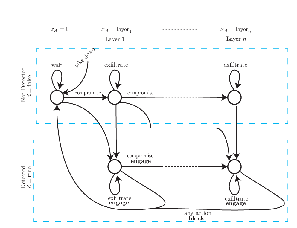
The network we consider consists of $n$ layers as illustrated in Figure 2. Each column in Figure 2 corresponds to a network layer, e.g., emails, databases, actuators and sensors, and etc.

The deceiver’s task here is to manipulate the infiltrator’s belief over whether he/she is being detected. The deceived infiltrator is hence convinced to take wrong actions due to the uncertainty about the infiltration progress. The deceiver has to manipulate the infiltrator’s belief and keep him $engage$ d in the network.

One way to represent the network security problem depicted in Figure 2 is to represent it by a one-sided POSG (to be described formally in the sequel), which is comprised of two parts. The upper-half corresponds to the states, wherein the presence of the infiltrator in the network has not been detected ( $d=\mathrm{false}$ ) and the deception mechanism cannot be implemented; whereas, the lower half corresponds to the case wherein the infiltrator is detected and therefore we can choose either actions $``\mathrm{engage}"$ or $``\mathrm{block}"$ .

The arrows illustrate the transitions in the game characterized by a transition function $T$ . We assume all transitions are deterministic, except transitions from $d=\mathrm{false}$ to $d=\mathrm{true}$ .

The infiltrator starts the attack at a computer outside the network $x_{A}=0$ . The infiltrator attempts to access computers in deeper layers by $compromise$ ing them. He/she also has the option to $wait$ at any layer, $takedown$ , which reveals the presence of the infiltrator and the infiltrator is forced to exit the network and restart the attack. Another course of action is to incur small amount of damage by $exfiltrate$ ing of data, which does not attract the deceiver’s attention.

The infiltrator does not receive observations for detection state $d$ , but is aware of $x_{A}$ (the network Layer being infiltrated). The deceiver has no information over the infiltrator until the infiltrator has been detected.

III Problem Statement

In this section, we first lay the formal foundations for POSGs, followed by a formal problem statement together with the underlying optimization problem.

III-A Foundations

A probability distribution over a finite or countably infinite set $X$ is a function $\mu\colon X\rightarrow[0,\,1]\subseteq\mathbb{R}$ with $\sum_{x\in X}\mu(x)=\mu(X)=1$ . The set of all distributions on $X$ is $\mathit{Distr}(X)$ . The support of a distribution $\mu$ is $\supp(\mu)=\{x\in X\,|\,\mu(x)>0\}$ . A distribution is Dirac if $|\!\supp(\mu)|=1$ . Let $V=\{x_{1},\ldots,x_{n}\}$ be a finite set of variables over the real numbers $\mathbb{R}$ . The set of multivariate polynomials over $V$ is $\mathbb{Q}[V]$ . An instantiation for $V$ is a function $u\colon V\rightarrow\mathbb{R}$ .

Definition 1 (SG)

A stochastic game (SG) is a tuple $G{}=(S_{\circ}{},S_{\Box}{},s_{\mathrm{I}}{},\mathit{Act},\mathcal{P}{})$ with a finite set $S=S_{\circ}\cup S_{\Box}$ of states, a set $S_{\circ}$ of Player 1 states, a set $S_{\Box}$ of Player 2 state, the initial state $s_{\mathrm{I}}\in S$ , a finite set $\mathit{Act}$ of actions, and a transition function $\mathcal{P}\colon S\times\mathit{Act}\rightarrow\mathit{Distr}(S)$ . We define costs using a state-action cost function $C:S\times\mathit{Act}\rightarrow\mathbb{R}_{\geq 0}$ .

A Markov decision process (MDP) is an SG in which $S_{\circ}=\emptyset$ , and consequently $S=S_{\Box}$ . A path of an SG $G$ is an (in)finite sequence $\pi=s_{0}\xrightarrow{a_{0}}s_{1}\xrightarrow{a_{1}}~s$ , where $s_{0}=s_{\mathrm{I}}$ , $s_{i}\in S$ , $a_{i}\in\mathit{Act}$ , and $\mathcal{P}(s_{i},a_{i})(s_{i+1})\neq 0$ for all $i\in\mathbb{N}$ . For finite $\pi$ , $\mathrm{last}(\pi)$ denotes the last state of $\pi$ . The set of (in)finite paths of $G$ is $\mathsf{Paths}_{\mathit{fin}}^{G}$ ( $\mathsf{Paths}^{G}$ ).

Definition 2 (SG strategy)

A strategy $\sigma$ for $G$ is a pair $\sigma=(\sigma_{1},\sigma_{2})$ of functions $\sigma_{i}\colon\{\pi\in\mathsf{Paths}_{\mathit{fin}}^{G}\mid\mathrm{last}(\pi)\in S_{i}\}\to\mathit{Distr}(\mathit{Act})$ such that for all $\pi\in\mathsf{Paths}_{\mathit{fin}}^{G}$ , $\{a\mid\sigma_{i}(\pi)(a)>0\}\subseteq\mathit{Act}\bigl(\mathrm{last}(\pi)\bigr)$ .

A Player- $i$ strategy $\sigma_{i}$ (for $i\in\{1,2\}$ ) is memoryless if $\mathrm{last}(\pi)=\mathrm{last}(\pi^{\prime})$ implies $\sigma_{i}(\pi)=\sigma_{i}(\pi^{\prime})$ for all $\pi,\pi^{\prime}\in\dom(\sigma_{i})$ . It is deterministic if $\sigma_{i}(\pi)$ is a Dirac distribution for all $\pi\in\dom(\sigma_{i})$ .

Definition 3 (One-sided POSG)

A one-sided partially observable stochastic game (POSG) is a tuple $\mathcal{G}{}=(G{},{Z}{},{O}{})$ , with $G{}=(S_{\circ}{},S_{\Box}{},s_{\mathrm{I}}{},\mathit{Act},\mathcal{P}{})$ the underlying SG of $\mathcal{G}$ , ${Z}$ a finite set of observations, and ${O}\colon S\rightarrow{Z}$ the observation function for Player 2.

A partially observable Markov decision process (POMDP) is an one-sided POSG in which $S_{\circ}=\emptyset$ , and consequently $S=S_{\Box}$ . In a POSG, players cannot make any choice when $|\mathit{Act}(s)|=1$ . Thus, for a POSG $\mathcal{G}$ with states $S_{\circ}\cup S_{\Box}$ , the POSG $\mathcal{G}^{\prime}$ with states $S_{\circ}^{\prime}=S_{\circ}\setminus\{s\in S_{\circ}\mid|\mathit{Act}(s)|=1\}$ and $S_{\Box}^{\prime}=S_{\Box}\cup\{s\in S_{\circ}\mid|\mathit{Act}(s)|=1\}$ and all transitions unchanged is equivalent w.r.t. the properties considered in the paper. Consequently, a POSG where one player never has a choice, i.e. $|\mathit{Act}(s)|=1,~\forall s\in S_{\circ}$ is also an MDP.

Without loss of generality, we assume Player 2 can observe its own available actions, thus $|\mathit{Act}(s)|=|\mathit{Act}(s^{\prime})|$ for all $s,s^{\prime}\in S_{\Box}$ with ${O}(s)={O}(s^{\prime})$ . Essentially, in a one-sided POSG, Player 1 has full observability, while Player 2 has only partial observability. We lift the observation function to paths: For $\pi=s_{0}\xrightarrow{a_{0}}s_{1}\xrightarrow{a_{1}}~ss_{n}\in\mathsf{Paths}_{\mathit{fin}}^{M}$ , the associated observation sequence is ${O}(\pi)={O}(s_{0})\xrightarrow{a_{0}}{O}(s_{1})\xrightarrow{a_{1}}~s{O}(s_{n})$ .

Definition 4 (POSG Strategy)

An observation-based strategy $\mathit{\sigma}=(\mathit{\sigma}_{1},\mathit{\sigma}_{2})$ for a one-sided POSG $\mathcal{G}$ is a strategy $(\mathit{\sigma}_{1},\mathit{\sigma}_{2})$ for the underlying SG $G$ such that $\mathit{\sigma}_{2}(\pi)=\mathit{\sigma}_{2}(\pi^{\prime})$ for all $\pi,\pi^{\prime}\in\mathsf{Paths}_{\mathit{fin}}^{\mathcal{G}}$ with ${O}(\pi)={O}(\pi^{\prime})$ . $\mathit{\sigma}_{1}$ is the Player 1 strategy, and $\mathit{\sigma}_{2}$ is the (observation-based) Player 2 strategy.

Applying the strategy $\mathit{\sigma}=(\mathit{\sigma}_{1},\mathit{\sigma}_{2})$ to a POSG $\mathcal{G}$ resolves all nondeterminism and partial observability, resulting in the induced Markov chain $\mathcal{G}^{\mathit{\sigma}}$ . In general, POSGs extend POMDPs and optimal strategies require infinite memory in general [5]. To represent observation-based strategies with finite memory, we use finite-state controllers (FSCs). If such an FSC has $n$ memory states, we speak of memory size $n$ for the underlying strategy $\mathit{\sigma}$ .

Definition 5 (FSC)

A finite-state controller (FSC) for a POMDP $\mathcal{M}$ is a tuple $\mathcal{A}=(N,n_{\mathrm{I}},\mathcal{\gamma},\mathcal{\delta})$ , where $N$ is a finite set of memory nodes, $n_{\mathrm{I}}\in N$ is the initial memory node, $\mathcal{\gamma}$ is the action mapping $\mathcal{\gamma}\colon N\times{Z}\rightarrow\mathit{Distr}(\mathit{Act})$ , and $\mathcal{\delta}$ is the memory update $\mathcal{\delta}\colon N\times{Z}\times\mathit{Act}\rightarrow\mathit{Distr}(N)$ . The set $\mathit{FSC}_{k}^{\mathcal{M}}$ denotes the set of FSCs with $k$ memory nodes, called $k$ -FSCs.

From a node $n$ and the observation $z$ in the current state of the POMDP, the next action $a$ is chosen from $\mathit{Act}(z)$ randomly as given by $\mathcal{\gamma}(n,z)$ . Then, the successor node of the FSC is determined randomly via $\mathcal{\delta}(n,z,a)$ .

Specifications. For a POSG $\mathcal{G}$ and a set $T\subseteq S$ of target states, we consider the maximal (or minimal) probability $\mathrm{Pr}_{\max}^{\mathcal{G}}(\lozenge T)$ ( $\mathrm{Pr}_{\min}^{\mathcal{G}}(\lozenge T)$ ) to reach $T$ , as well as the maximal (or minimal) expected cost $\mathrm{EC}_{\max}^{\mathcal{G}}(\lozenge T)$ ( $\mathrm{EC}_{\min}^{\mathcal{G}}(\lozenge T)$ ). For a probability bound $\lambda\in[0,1]$ and an expected cost bound $\kappa\in\mathbb{R}$ , we also consider specifications of the form $\varphi=\mathbb{P}_{\leq\lambda}(\lozenge T)$ and $\psi=\mathrm{EC}_{\leq\kappa}(\lozenge T)$ , where the probability or the expected cost to reach $T$ shall be at most $\lambda$ or $\kappa$ , respectively. The specification $\varphi$ is satisfied for a strategy $\mathit{\sigma}=(\mathit{\sigma}_{1},\mathit{\sigma}_{2})$ and the POSG $\mathcal{G}$ if the probability $\mathrm{Pr}^{\mathcal{G}^{\mathit{\sigma}}}(\lozenge T)$ of reaching a target state in $\mathcal{G}^{\mathit{\sigma}}$ is at most $\lambda$ , denoted by $\mathcal{M}^{\mathit{\sigma}}\models\varphi$ . This satisfaction relation is analogous for expected cost.

Sufficiently strong strategies. For a POSG $\mathcal{G}$ and a property $\varphi$ , a strategy $\sigma_{1}$ for Player 1 is called sufficiently strong for $\varphi$ against a set $\mathcal{S}\subseteq{\Sigma}_{2}$ of strategies for Player 2, if for each strategy $\sigma_{2}\in\mathcal{S}$ of Player 2, $\mathcal{G}^{(\sigma_{1},\sigma_{2})}\models\varphi$ .

III-B Deception Games

Definition 6 (Deception Game)

A deception game is a one-sided POSG, where Player 1 (with full observability) is called the infiltrator and Player 2 (with partial observability) is called the deceiver. See Figure 3 for an illustration of the robust deception problem.

In the POSG that captures the motivating example, we identify the target states $T\subseteq S$ as the states that correspond to Layer $n$ . The goal is to deceive the infiltrator such that the expected cost to reach those states is maximized. We state the formal problem.

Problem 1: Given a deception game

\mathcal{G}{}=(G{},{Z}{},{O}{})

, a set of target states

T\subseteq S

, memory bound

n

, and specification

\varphi=\mathrm{EC}_{\min}^{\mathcal{G}}(\lozenge T)

, compute a sufficiently strong strategy for the deceiver, against infiltration-strategies with memory

n^{\prime}\leq n

Fig. 3: The Robust Deception Problem.

The straightforward solution to Problem 1 can be given by solving a robust mixed-integer linear program (MILP) with variables as described next.

For $s_{\circ}\in S_{\circ}$ and each action $a\in\mathit{Act}$ , the strategy variable $\delta^{s_{\circ}}_{a}\in\{0,1\}$ denotes which action is active in each state $s_{\circ}$ . If $\delta^{s_{\circ}}_{a}=1$ , then Player 1 takes action $a$ in state $s_{\circ}$ . For $s_{\circ}\in S_{\circ},$ and $s_{\Box}\in S_{\Box}$ , the cost variables $c_{s_{\circ}}\geq 0$ $c_{s_{\Box}}\geq 0$ and represent the expected cost of reaching $T\subseteq S$ . $M$ is a large constant that automatically satisfies the constraints in (6) and (7) if $\delta^{s_{\circ}}_{a}=0$ , which means the deceiver does not select action $a$ in state $s_{\circ}$ . $\gamma\in[0,1)$ is the discount factor to ensure that we have finite expected cost.

We then have the following robust MILP that solves Problem 1.

		$\displaystyle\underset{c_{s_{\circ}},c_{s_{\Box}},\delta^{s_{\circ}}_{a}}{\text{minimize}}\quad c_{s_{\mathrm{I}}}$		(1)
		subject to
		$\displaystyle c_{s}=0,\quad\forall s\in T$		(2)
		$\displaystyle\sum_{a\in\mathit{Act}}\sigma^{z}_{a}=1,\quad\forall z\in{Z}$		(3)
		$\displaystyle\sum_{a\in\mathit{Act}}\delta^{s_{\circ}}_{a}=1,\quad\forall s_{\circ}\in S_{\circ}$		(4)
		$\displaystyle c_{s_{\Box}}=C(s_{\Box},a)+\sum_{a\in\mathit{Act}}\sigma^{{O}(s_{\Box})}_{a}~\sum_{s^{\prime}_{\circ}\in\lx@sectionsign_{\circ}}\mathcal{P}(s_{\Box},a,s^{\prime}_{\circ})~c_{s^{\prime}_{\circ}},$
		$\displaystyle\qquad\qquad\qquad\qquad\forall s_{\Box}\in S_{\Box}\setminus T,\,\forall\sigma^{{O}(s_{\Box})}_{a}\in\sigma_{2}$		(5)
		$\displaystyle c_{s_{\circ}}\geq C(s_{\circ},a)+\gamma~\sum_{s^{\prime}_{\Box}\in S_{\Box}}\mathcal{P}(s_{\circ},a,s^{\prime}_{\Box})~c_{s^{\prime}_{\Box}}-M~(1-\delta^{s_{\circ}}_{a}),$
		$\displaystyle\qquad\qquad\qquad\qquad\forall s_{\circ}\in S_{\circ}\setminus T,\,\forall a\in\mathit{Act}$		(6)
		$\displaystyle c_{s_{\circ}}\leq C(s_{\circ},a)+\gamma~\sum_{s^{\prime}_{\Box}\in S_{\Box}}\mathcal{P}(s_{\circ},a,s^{\prime}_{\Box})~c_{s^{\prime}_{\Box}}+M~(1-\delta^{s_{\circ}}_{a}),$
		$\displaystyle\qquad\qquad\qquad\qquad\forall s_{\circ}\in S_{\circ}\setminus T,\,\forall a\in\mathit{Act}.$		(7)

The objective in (1) minimizes the expected cost of the deceiver. We assign the expected cost of the states in the target set to 0 by the constraints in (2). We ensure that the strategies of the infiltrator and the deceiver are well-defined with the constraints in (3) and (4). The constraints in (5)–(7) gives the computation for the expected cost in the states of the POSG.

Proposition 1

The robust MILP in (1) – (7) computes the maximal probability of reaching $T$ under a (maximizing) randomized memoryless observation-based strategy.

Unfortunately, robust MILP’s are notoriously hard to solve, except in special cases of small problems with few constraints [12] or only having binary variables [3]. Recently, [26] proposes a heuristic relaxation for robust MILP’s using the affinely adjustable robust counterpart [2]. However, large robust MILP’s, such as the robust MILP above for Problem 1, remain intractable in general.

IV Tractable Approach

Fig. 4: Computing Infiltration Strategies for Stage 1.

In this section, we propose a two-stage approach for solving Problem 1. We begin by giving some key formalisms.

IV-1 Parametric MDPs

Instead of having fixed probabilities in the transition function of an MDP, we allow to describe the transition probabilities of an MDP as polynomials over a fixed set of variables. By having different values for the parameters, we can induce different MDPs.

Definition 7 (pMDP)

A parametric Markov decision process (pMDP) $M$ is a tuple $M{}=(S{},\,s_{\mathrm{I}}{},\mathit{Act}{},V,\mathcal{P}{})$ with a finite (or countably infinite) set $S$ of states, initial state $s_{\mathrm{I}}\in S$ , a finite set $\mathit{Act}$ of actions, a finite set $V$ of parameters, and a transition function $\mathcal{P}\colon S\times\mathit{Act}\times S\rightarrow\mathbb{Q}[V]$ .

Applying an instantiation $u\colon V\to\mathbb{R}$ to a pMDP $M$ , denoted $M[u]$ , replaces each polynomial $\mathbb{Q}[V]$ in $M$ by $\mathbb{Q}[u]$ . $M[u]$ is also called the instantiation of $M$ at $u$ . Instantiation $u$ is well-defined for $M$ if the replacement yields probability distributions, i. e., if $M[u]$ is an MDP.

Definition 8 (pMDP Synthesis Problem)

Given a pMDP $M$ and a property $\varphi$ , the synthesis problem is to compute an instantiation $u$ such that $M[u]\models\varphi$ , if one exists.

The pMDP synthesis problem amounts to solving the following NLP.

		$\displaystyle\underset{c_{s},V}{\text{maximize}}\quad c_{s_{\mathrm{I}}}$		(8)
		subject to
		$\displaystyle c_{s_{\mathrm{I}}}\leq\kappa,$		(9)
		$\displaystyle c_{s}=0,\quad\forall s\in T$		(10)
		$\displaystyle\mathcal{P}(s,a,s^{\prime})\geq 0,\quad\forall s,s^{\prime}\in S,\,\forall a\in\mathit{Act}$		(11)
		$\displaystyle\sum_{s^{\prime}\in S}\mathcal{P}(s,a,s^{\prime})=1,\quad\forall s\in S,\,\forall a\in\mathit{Act}$		(12)
		$\displaystyle c_{s}\geq C(s,a)+\gamma\sum_{s^{\prime}\in S}\mathcal{P}(s,a,s^{\prime})~c_{s^{\prime}},$		(13)
		$\displaystyle\qquad\qquad\qquad\qquad\forall s\in S\setminus T,\,\forall a\in\mathit{Act}.$

For $s\in S$ , the cost variable $c_{s}\geq 0$ represents an upper bound of expected cost of reaching target set $T\subseteq S$ , and the parameters in set $V$ enter the NLP as part of the functions from $\mathbb{Q}[V]$ in the transition function $\mathcal{P}$ .

One particular efficient method for finding parameter instantiations is given in [6], which solves the NLP in (8)–(13) via a reformulation to a convex-concave programming problem [23] and an efficient integration of model checking calls to improve its performance. We are now ready to outline the proposed tractable approach.

IV-A Stage 1: Computing Infiltration Strategies

In this section, we are given a POSG and are interested in computing several sufficiently strong infiltrator strategies. For an overview of the approach in Stage 1, see Figure 4.

Task 1

Given a POSG $\mathcal{G}$ , compute several sufficiently strong strategies for the infiltrator.

We detail the approach first for an infiltrator that uses memoryless strategies. We then generalize the approach to any (finite but fixed) amount of memory for the infiltrator. The approach extends the reduction from POMDPs to pMCs in [19].

IV-A1 Memoryless strategies

A memoryless strategy maps observations to distributions over actions. Equivalently, such strategy maps observation-action pairs to probabilities (ObAct-probabilities). Any memoryless strategy is uniquely defined by its ObAct-probabilities. Instead of finding suitable strategies for the infiltrator, we can thus reformulate our approach to finding suitable ObAct-probabilities. Hence, a suitable strategy can be described as parameter values that satisfy the property of an pMDP. To find the ObAct-probabilities, we construct an equivalent pMDP as illustrated in the following example.

(a) a POSG

(b) the pMDP

Fig. 5: From POSG to pMDP

Example 1

Consider the POSG in Fig. 5(a). The states for Player 1 are given by circles. Similarly, the rectangles depict the states for Player 2. We indicate the actions from the states with solid lines to black dots. The corresponding probabilities from the black dots give the probability of transitioning to the next state. Thus, we draw dashed (direct) lines from the Player 1 (Player 2) nodes. The colors of states indicate the corresponding observations.

The corresponding pMDP for a memoryless, observation-based strategy for player 2 is given in Fig. 5(b). The actions of player 1 are unchanged. As there is no more nondeterminism in the states of player 2, we can also view these states as player 1 states. Moreover, to avoid clutter, we omit action indications. Consider state $s_{3}$ with outgoing action $a_{2}$ , which leads with probability $1$ to $s_{4}$ . Under a strategy, we take this action with probability $q$ : Thus, in the pMDP there is an arc with probability $q$ from $s_{3}$ to $s_{4}$ . If we take action $a_{2}$ with probability $q$ , we take action $a_{1}$ with probability $1{-}q$ . The same probabilities for taking the actions have to hold in state $s_{1}$ . Observe that the probabilities are not immediately reflected, as there are two paths from $s_{1}$ to $s_{2}$ . The parameters in $s_{0}$ are different. Indeed, there are $2$ parameters as there are three actions to take.

We formalize the construction below for situations, where the infiltrator has three available actions in each state, to simplify the notation.

Definition 9

Given a POSG $\mathcal{G}{}=(G{},{Z}{},{O}{})$ with SG $G{}=(S_{\circ}{},S_{\Box}{},s_{\mathrm{I}}{},\mathit{Act},\mathcal{P}{})$ . Let $\forall s\in S_{\Box}~|\mathit{Act}(s)|=3$ . Without loss of generality, refer to $\mathit{Act}(s)=\{a_{1},a_{2},a_{3}\}$ if $s\in S_{\Box}$ . The pMDP $M{{}^{\prime}}=(S{{}^{\prime}},\,s_{\mathrm{I}}{{}^{\prime}},\mathit{Act}{{}^{\prime}},V,\mathcal{P}{{}^{\prime}})$ is the corresponding pMDP for POSG $\mathcal{G}$ , if $S^{\prime}=S_{\circ}\cup S_{\Box}$ , $s_{\mathrm{I}}^{\prime}=s_{\mathrm{I}}$ , $\mathit{Act}^{\prime}=\mathit{Act}\cup\{\bot\}$ , $V=\{p^{z}_{1},p^{z}_{2}\mid z\in{Z}\}$ and $\mathcal{P}^{\prime}(s,a,s^{\prime})=$

\begin{cases}\mathcal{P}(s,a,s^{\prime})&\text{ if }s\in S_{\circ}\\ \sum_{i=1}^{3}f^{z}_{i}\mathcal{P}(s,a_{i},s^{\prime})&\text{ if }s\in S_{\Box},a=\bot,z={O}(s)\\ 0&\text{otherwise.}\end{cases}

where $f^{z}_{i}$ denotes $p_{1}^{z}$ , $p_{2}^{z}$ and $1-p_{1}^{z}-p_{2}^{z}$ , respectively.

The construction is straightforward to adapt to a varying number of actions per state: Indeed, we just need additional variables $p^{z}_{i}$ indicating that we take action $i$ in a state with observation $z$ .

We denote the memoryless strategy $\mathsf{IStrat}(u)$ for the infiltrator in the deception game that is induced by a valuation $u$ in the infiltration-pMDP.

Theorem 1

Given a deception game $\mathcal{G}$ , with its corresponding infiltration-pMDP $\mathcal{I}(\mathcal{G})$ , and a property $\varphi$ . Let $u$ be a solution for the pMDP synthesis problem for the property $\varphi$ . Then $\mathsf{IStrat}(u)$ is a sufficiently strong strategy for the infiltrator on the $G$ and $\varphi$ .

IV-A2 Adding Memory to the Infiltrator Strategy

The ideas for the synthesis of memoryless strategies can be lifted to a finite ( $k$ ) memory setting. We apply an $k-$ unfolding of the POSG, and then search for a memoryless infiltrator strategy. The idea is to create $k$ copies of the POSG, and allow the infiltrator to freely switch between copies. The different copies correspond to the internal memory of the infiltrator.

IV-B Stage 2: Computing a Robust Deception Strategy

In this section, we assume that the deceiver obtained $N$ strategies for the infiltrator. Then, the task of the deceiver is to compute a strategy that minimizes the worst-case expected cost $\psi=\mathrm{EC}_{\leq\kappa}(\lozenge T)$ to reach a target set $T$ against any of the $N$ infiltration strategies under all deceiver policies. If the deception strategy has access to the memory node of the infiltration strategy, we call the infiltration memory transparent.

Task 2

Given a deception game, a set of transparent infiltration strategies, compute a deception strategy that is optimal under all deception strategies against the set of infiltration strategies.

IV-B1 Deceiving against Transparent-Memory Infiltrator Strategies

We focus on memoryless infiltration strategies. Memoryless infiltration strategies are the most prominent transparent memory case, and for transparent memory, each finite memory strategy can be reduced to a memoryless strategy by unfolding the memory into the MDP, as in Stage 1.

To compute a robust deception strategy against transparent infiltrator strategies, we remove the uncertain constraints of the robust MILP in (1) – (7) by using the infiltrator strategies that we obtained in Stage 1. Then, we reduce the problem of synthesizing a robust deception strategy problem to solving an MILP instead of solving a robust MILP. We now give the details of the resulting MILP with the infiltrator strategies.

We define the following variables for the following MILP: For $s_{\circ}\in S_{\circ}$ , $s_{\Box}\in S_{\Box}$ , and for each infiltrator strategy $\sigma^{i,{O}(s_{\Box})},i=1,\ldots,N$ , the cost variables $~c^{i}_{s_{\circ}}\geq 0$ and $~c^{i}_{s_{\Box}}\geq 0$ give the expected cost of reaching $T\subseteq S$ for each infiltrator strategies. For $s_{\circ}\in S_{\circ}$ and each action $a\in\mathit{Act}$ , the strategy variable $\delta^{s_{\circ}}_{a}\in\{0,1\}$ denotes which action is active in each state $s_{\circ}$ . If $\delta^{s_{\circ}}_{a}=1$ , then the deceiver takes action $a$ in state $s_{\circ}$ .

For observation $z\in{Z}$ , for each action $a\in\mathit{Act}$ and for each infiltrator strategy $\sigma^{i,{O}(s_{\Box})},i=1,\ldots,N$ , $\sigma^{i,{O}(s_{\Box})}_{a}$ represents the probability of choosing action $a\in\mathit{Act}$ upon observation $z$ for each strategy of Player 2. Similar to the Problem 1, $M$ is a large constant that automatically satisfies the constraints in (18) and (19) if $\delta^{s_{\circ}}_{a}=0$ , which means the deceiver does not select action $a$ in state $s_{\circ}$ .

We thus have the following MILP:

		$\displaystyle\underset{c^{i}_{s_{\circ}},c^{i}_{s_{\Box}},\delta^{s_{\circ}}_{a}}{\text{minimize}}\;\;\underset{i}{\text{max}}\quad r^{i}_{s_{\mathrm{I}}}$		(14)
		subject to
		$\displaystyle~c^{i}_{s}=0,\quad\forall s\in T,~i=1,\ldots,N$		(15)
		$\displaystyle\sum_{a\in\mathit{Act}}\delta^{s_{\circ}}_{a}=1,\quad\forall s_{\circ}\in S_{\circ}$		(16)
		$\displaystyle~c^{i}_{s_{\Box}}=C(s_{\Box},a)+\sum_{a\in\mathit{Act}}\sigma^{i,{O}(s_{\Box})}_{a}\sum_{s^{\prime}_{\circ}\in\lx@sectionsign_{\circ}}\mathcal{P}(s_{\Box},a,s^{\prime}_{\circ})~c^{i}_{s^{\prime}_{\circ}},$
		$\displaystyle\qquad\qquad\qquad\qquad\forall s_{\Box}\in S_{\Box}\setminus T,~i=1,\ldots,N$		(17)
		$\displaystyle~c^{i}_{s_{\circ}}\geq C(s_{\circ},a)+\gamma\sum_{s^{\prime}_{\Box}\in S_{\Box}}\mathcal{P}(s_{\circ},a,s^{\prime}_{\Box})~c^{i}_{s^{\prime}_{\Box}}-M(1-\delta^{s_{\circ}}_{a}),$
		$\displaystyle\qquad\qquad\qquad\qquad\forall s_{\circ}\in S_{\circ}\setminus T,\,\forall a\in\mathit{Act},~i=1,\ldots,N$		(18)
		$\displaystyle~c^{i}_{s_{\circ}}\leq C(s_{\circ},a)+\gamma\sum_{s^{\prime}_{\Box}\in S_{\Box}}\mathcal{P}(s_{\circ},a,s^{\prime}_{\Box})~c^{i}_{s^{\prime}_{\Box}}+M(1-\delta^{s_{\circ}}_{a}),$
		$\displaystyle\qquad\qquad\qquad\qquad\forall s_{\circ}\in S_{\circ}\setminus T,\,\forall a\in\mathit{Act},~i=1,\ldots,N.$		(19)

The objective in (14) minimize the worst-case expected cost of deception against the infiltrator strategies. The constraint in (15) sets the expected cost of the states in $T$ to be 0. Constraint (16) ensures that the deceiver picks one of the actions in $\mathit{Act}$ for each state in $S_{\circ}$ . The constraints (17)–(19) concerns the cost computation for each state in $S_{\circ}$ , and $S_{\Box}$ .

By solving the MILP in (14) – (19), we construct a strategy for the deceiver that is sufficiently strong against infiltrator strategies. By construction, we have the following theorem.

Theorem 2

The MILP in (14) – (19) computes a sufficiently strong strategy for the deceiver against $N$ strategies of the infiltrator.

States		Actions		loss ( $l$ )
Infiltrator’s Position ( $x_{A}$ )	Detection mode ( $d$ )	Infiltrator ( $a_{I}$ )	Deceiver ( $a_{D}$ )
$any$	false	compromise	–	$-2$
$\mathrm{layer}_{i}$	false	exfiltrate	–	$15i$
$\mathrm{layer}_{i}$	false	takedown	–	$25i$
$any$	true	compromise	engage	$-4$
$\mathrm{layer}_{i}$	true	exfiltrate	engage	$-2$
$\mathrm{layer}_{i}$	true	takedown	engage	$25i$
$any$	true	compromise	block	$-2$
$any$	true	exfiltrate	block	$0$
$any$	true	takedown	block	$0$

TABLE I: The losses incurred when both players take simultaneous actions at different states.

V Numerical Experiments

At this point, we are ready to return to the motivating example. We define the expected discounted cost for the deceiver corresponding to each action the infiltrator takes by

L=\sum_{t=1}^{\infty}\gamma^{t-1}\cdot l^{(t)},

where $\gamma$ is the discount factor and $l^{(t)}$ denotes the loss at stage $t$ . For this example, the specification of the deceiver is $\psi=\mathrm{EC}_{\min}$ , which is to minimize $L$ against all infiltration strategies. Table I outlines the elements of the one-sided deception POSG. Note that since the players take actions concurrently, the costs depend on their joint actions. Furthermore, some of the costs are dependent on the layer index $i$ the infiltrator has accessed. For more details about the example, the interested reader is referred to [18].

We first describe our results on a 4-layer network, given by [18]. Then, we demonstrate our approach on a 12-layer network. For each network, we first compute infiltration strategies for the deceiver using the approach in Stage 1. Then, using these infiltration strategies, we compute a robust deceiver strategy, which is given by in Stage 2. The arising pMDP problems from Stage 1 is solved using the approach in [6]. We solve the MILP problems from Stage 2 using the MILP solver GUROBI [13].

For the 4-layer network, we first construct the one-sided deception POSG with 2 memory nodes. The POSG consists of 49 states, 8 action choices for the deceiver, and 34 actions for the infiltrator. After computing an optimal deceiver strategy, the worst-case induced cost against $1000$ infiltration strategies obtained from the approach in Stage 1 is 282.22. The obtained cost is comparable to the approach given by [18]. The procedure for obtaining the infiltration strategies took 193.29 seconds, and time to compute the optimal deceiver strategy is 216.92 seconds.

The optimal deceiver strategy that we obtained is to engage the infiltrator in first 2 layers, then blocking the infiltrator in the last layers. This seems to be beneficial compared to always blocking the infiltrator, which leads to a worst-case expected cost of 341.72, and always engaging the infiltrator, which leads to a worst-case expected cost of 304.05.

We also give the results with different number of infiltrator strategies on a 4-layer and 12-layer network in Table II. The expected cost of the defender increases with increasing number of infiltrator strategies in all cases. Also, by increasing number of layers, the deceiver can craft an optimal strategy in a 12-layer network that incurs a less expected loss compared to the optimal strategy in a 4-layer network. However, if the deceiver always blocks or engages, the expected cost increases with increasing number of layers.

Number of infiltrator strategies	10	100	1000
Number of Layers & deceiver strategies	10	100	1000
4 & Always engage	260.17	297.45	304.05
4 & Always block	246.12	286.19	341.72
4 & Optimal	228.64	256.81	282.22
12 & Always engage	277.71	301.46	313.91
12 & Always block	256.39	294.65	308.12
12 & Optimal	217.76	239.71	261.49

TABLE II: Expected loss of the defender in various scenarios.

VI Conclusion

We presented an approach to solve a partially observable stochastic game (POSG), where one of the player has full observability over the states, and the other player only has partial observability. We formulated the problem as a robust mixed-integer linear program, which is intractable to solve in general. To obtain a more scalable approach, we computed a robust optimal strategy for the deceiver by synthesizing a set of infiltration strategies using parameter synthesis in parametric Markov decision processes. Using a mixed-integer linear program and the infiltration strategies, we computed the robust deception strategy. We illustrated our approach on a POSG model for network security and we showed that we can handle larger networks compared to the previous approaches in the literature.

Future work concerns removing the transparency approach, which means the deceiver has access to the memory node of the infiltration strategy, if the infiltration strategy is memory-based. Also, we will explore some of the recent methods to solve mixed-integer linear problems proposed in the literature, such as methods proposed in [9, 10].

References

[1] T. Basar and Geert J. Olsder. Dynamic noncooperative game theory, volume 23. Siam, 1999.
[2] A. Ben-Tal, A. Goryashko, E. Guslitzer, and A. Nemirovski. Adjustable robust solutions of uncertain linear programs. Mathematical Programming, 99(2):351–376, 2004.
[3] Dimitris Bertsimas and Melvyn Sim. Robust discrete optimization and network flows. Mathematical programming, 98(1-3):49–71, 2003.
[4] E. Byres and J. Lowe. The myths and facts behind cyber security risks for industrial control systems. In Proceedings of the VDE Kongress, volume 116, pages 213–218, 2004.
[5] Krishnendu Chatterjee, Martin Chmelík, and Mathieu Tracol. What is decidable about partially observable markov decision processes with $\omega$ -regular objectives. Journal of Computer and System Sciences, 82(5):878–911, 2016.
[6] Murat Cubuktepe, Nils Jansen, Sebastian Junges, Joost-Pieter Katoen, and Ufuk Topcu. Synthesis in pMDPs: A tale of 1001 parameters. CoRR, abs/1803.02884, 2018.
[7] Donald C Daniel and Katherine L Herbig. Strategic Military Deception: Pergamon Policy Studies on Security Affairs. Elsevier, 2013.
[8] Dorothy Elizabeth Robling Denning. Information warfare and security, volume 4. Addison-Wesley Reading, MA, 1999.
[9] Souradeep Dutta, Susmit Jha, Sriram Sanakaranarayanan, and Ashish Tiwari. Output range analysis for deep neural networks. arXiv preprint arXiv:1709.09130, 2017.
[10] Souradeep Dutta, Susmit Jha, Sriram Sankaranarayanan, and Ashish Tiwari. Learning and verification of feedback control systems using feedforward neural networks. IFAC-PapersOnLine, 51(16):151–156, 2018.
[11] R. Emery-Montemerlo, G. Gordon, J. Schneider, and S. Thrun. Approximate solutions for partially observable stochastic games with common payoffs. In Autonomous Agents and Multiagent Systems, 2004. AAMAS 2004. Proceedings of the Third International Joint Conference on, pages 136–143. IEEE, 2004.
[12] Kai-Simon Goetzmann, Sebastian Stiller, and Claudio Telha. Optimization over integers with robustness in cost and few constraints. In International Workshop on Approximation and Online Algorithms, pages 89–101. Springer, 2011.
[13] Gurobi Optimization, Inc. Gurobi optimizer reference manual. http://www.gurobi.com, 2013.
[14] Ernst Moritz Hahn, Tingting Han, and Lijun Zhang. Synthesis for pctl in parametric markov decision processes. In NASA Formal Methods Symposium, pages 146–161. Springer, 2011.
[15] E. A Hansen, D. S. Bernstein, and S. Zilberstein. Dynamic programming for partially observable stochastic games. In AAAI, volume 4, pages 709–715, 2004.
[16] J. P. Holdren and E. S. Lander. Big data and privacy: a technological perspective. Report to the President (Executive Office of the President President’s Council of Advisors on Science and Technology), 2014.
[17] K. Horák, B. Bosanskỳ, and M. Pechoucek. Heuristic search value iteration for one-sided partially observable stochastic games. In AAAI, pages 558–564, 2017.
[18] K. Horák, Q. Zhu, and B. Bošanskỳ. Manipulating adversary’s belief: A dynamic game approach to deception by design for proactive network security. In International Conference on Decision and Game Theory for Security, pages 273–294. Springer, 2017.
[19] Sebastian Junges, Nils Jansen, Ralf Wimmer, Tim Quatmann, Leonore Winterer, Joost-Pieter Katoen, and Bernd Becker. Finite state controllers for pomdps via parameter synthesis. In UAI, 2018.
[20] D. Kuipers and M. Fabro. Control systems cyber security: Defense in depth strategies. United States. Department of Energy, 2006.
[21] A. Kumar and S. Zilberstein. Dynamic programming approximations for partially observable stochastic games. In FLAIRS Conference, 2009.
[22] D. Kushner. The real story of Stuxnet. IEEE Spectrum, 3(50):48–53, 2013.
[23] Thomas Lipp and Stephen Boyd. Variations and extension of the convex–concave procedure. Optimization and Engineering, 17(2):263–287, 2016.
[24] M. H. Manshaei, Q. Zhu, T. Alpcan, T. Basar, and J. Hubaux. Game theory meets network security and privacy. ACM Computing Surveys (CSUR), 45(3):25, 2013.
[25] K. D. Mitnick and W. L. Simon. The art of deception: Controlling the human element of security. John Wiley & Sons, 2011.
[26] Jean Pauphilet, Diego Kiner, Damien Faille, and Laurent El Ghaoui. A tractable numerical strategy for robust milp and application to energy management. In Decision and Control (CDC), 2016 IEEE 55th Conference on, pages 1490–1495. IEEE, 2016.
[27] Lance Spitzner. Honeypots: tracking hackers, volume 1. Addison-Wesley Reading, 2003.
[28] Colin Tankard. Advanced persistent threats and how to monitor and deter them. Network security, 2011(8):16–19, 2011.
[29] Q. Zhu and T. Basar. Game-theoretic methods for robustness, security, and resilience of cyberphysical control systems: games-in-games principle for optimal cross-layer resilient control systems. IEEE control systems, 35(1):46–65, 2015.