跳到论文正文
W Papers独立论文阅读器 arXiv:1809.11071 论文正文 计算阅读时间 · 0%
引用这篇论文根据当前论文元数据生成,正式投稿前建议核对。


License: arXiv.org perpetual non-exclusive license
arXiv:1809.11071v1 [cond-mat.quant-gas] 28 Sep 2018

Phonon-mediated Casimir interaction between finite mass impurities

Andrei I. Pavlov Affiliation: Institute for Theoretical Solid State Physics, Leibniz-Institut für Festkörper- und Werkstoffforschung IFW-Dresden, D-01169 Dresden, Helmholtzstraße 20, Germany    Jeroen van den Brink Affiliation: Institute for Theoretical Solid State Physics, Leibniz-Institut für Festkörper- und Werkstoffforschung IFW-Dresden, D-01169 Dresden, Helmholtzstraße 20, Germany    Dmitri V. Efremov Affiliation: Institute for Theoretical Solid State Physics, Leibniz-Institut für Festkörper- und Werkstoffforschung IFW-Dresden, D-01169 Dresden, Helmholtzstraße 20, Germany
Abstract

The Casimir effect, a two-body interaction via vacuum fluctuations, is a fundamental property of quantum systems. In solid state physics it emerges as a long-range interaction between two impurity atoms via virtual phonons. In the classical limit for the impurity atoms in DD dimensions the interaction is known to follow the universal power-law U⁡(r)∼r−DU(r)\sim r^{-D}. However, for finite masses of the impurity atoms on a lattice, it was predicted to be U⁡(r)∼r−2​D−1U(r)\sim r^{-2D-1} at large distances. We examine how one power-law can change into another with increase of the impurity mass and in presence of an external potential. We provide the exact solution for the system in one-dimension. At large distances indeed U⁡(r)∼r−3U(r)\sim r^{-3} for finite impurity masses, while for the infinite impurity masses or in an external potential it crosses over to U⁡(r)∼r−1U(r)\sim r^{-1} . At short distances the Casimir interaction is not universal and depends on the impurity mass and the external potential.

pacs
42.50.Lc, 63.20.Ls, 63.22.-m, 63.70.+h

Casimir in his pioneering work [1] has shown that a change of the zero-point energy due to a perturbation of the electromagnetic fluctuations by two neutral metallic plates, leads to observable forces between these plates. In fact, this is only one example of the broad class of phenomena, which are based on the concept of perturbation of the long-range fluctuations, e.g. Goldstone modes in the media with broken symmetry. Nowadays this effect, named after Casimir, can be encountered in various fields of physics, chemistry and biology [2, 3, 4, 5, 6, 7, 8]. For instance, in high energy physics the existence of Casimir effect sets natural constraints on the Yukawa forces, appearing due to the exchange of light elementary particles and/or extra- dimensional physics [9]. In cosmology the Casimir effect helps to interpret the cosmological constant for a scalar field [10, 11, 12]. In chemistry, in particular, it is used to explain the interactions of molecules [13, 14]. In biology the Casimir interaction is for instance found to be responsible for organization of the bilayer structure of cell membranes [15].

In condensed matter physics the effect of the Casimir interaction is extensively discussed with respect to interaction of conducting surfaces [16], graphene and conducting plates [17], mesoscopic particles in a critical fluid through critical fluctuations [18] and ultracold atomic gases [19, 20, 21]. In the latter case it is possible to study the Casimir interaction in ultraclean bosonic or fermionic gases on tunable lattices with tunable spatial dimensionality and interaction strength. In this context one dimensional setups attract the most attention since the fluctuations are the strongest in 1D.

Precisely this situation was considered in [19, 20, 21]. The authors studied the interaction between two static impurities due to perturbation of phonon spectra in a Luttinger liquid. Since the mechanism is similar to the one proposed by Casimir, we hereafter denote it as the Casimir interaction. The examination of the energy of zero-point motion of the Luttinger liquid in the presence of two impurities yielded the Casimir interaction U(r)∼−1/rU(r)\sim-1/r. This dependence can be easily understood considering the zero-point energy of phonons in a potential well formed by two static impurities. The direct calculation leads to the following expression for the Casimir interaction [22, 23]:

U⁡(r)=−c​π24​r,U(r)=-\frac{c\pi}{24r}, (1)

(here and below we use ℏ=1\hbar=1).

At the same time, for two dynamical impurities which can move inside the medium, Schecter and Kamenev in [24] proposed an essentially different rr-dependence, U⁡(r)=−m​c2​Γ1​Γ232​π​ξ3r3U(r)=-mc^{2}\frac{\Gamma_{1}\Gamma_{2}}{32\pi}\frac{\xi^{3}}{r^{3}}, where mm is the mass of particles in the fluid, cc is the sound velocity, ξ=1/m​c\xi=1/mc and the dimensionless parameters Γ1,2\Gamma_{1,2} are impurity-phonon scattering amplitude. How the power law for dynamic impurities transforms to another for the static impurities is an open question.

To address this question we investigate a model of a harmonic crystal lattice with embedded two impurity neutral atoms. It is arguably the simplest model in which one can tune impurities continuously from dynamic to static and keep track of the evolution of the Casimir interaction. In this model the Casimir interaction emerges naturally between two impurity atoms as soon as their mass is different from the masses of the lattice atoms or an external potential is applied. We find that the Casimir interaction has different asymptotics in these two cases. In the former one, for any finite mass of the impurity atoms the Casimir interaction tends to the 1/r31/r^{3}-law at large distances in agreement with [24]. At the same time, in the limit of infinity mass the long range asymptotic tends to 1/r1/r in agreement with [19, 20, 21]. In the case of an external potential the asymptotics is always 1/r1/r.

Our letter is organized as follows. Firstly we consider two neutral impurity atoms embedded in a harmonic crystal lattice. Using the exact diagonalization method we show that the power law at short distances strongly deviates from 1/r31/r^{3} and the characteristic distance of the crossover to 1/r31/r^{3}-law depends on the masses of the impurity atoms. Then we provide the exact solution for the model and formulate the continuum model. In the second part of the article formulate and exactly solve the model of two impurity atoms in an external harmonic potential. We show that the model is nonperturbative and has 1/r1/r asymptotic behavior. Finally, we provide a discussion of the obtained results and conclusion.

Refer to caption

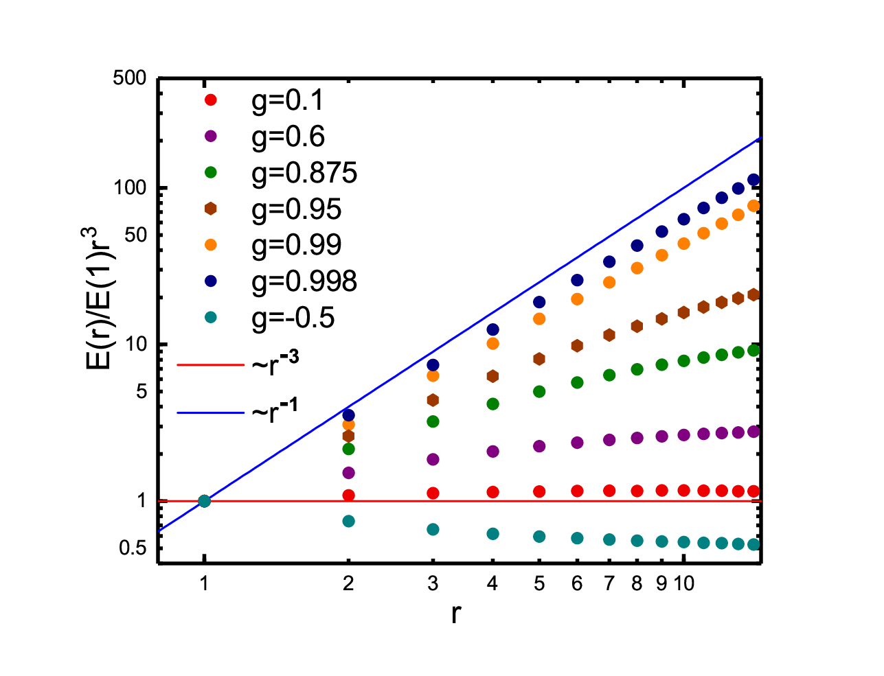
Figure 1: Normalized Casimir interaction Ueff​(r)U_{\rm{eff}}(r) calculated for a chain of 200 atoms with two impurity atoms with various masses: Red dots - g=0.1g=0.1 (M/m=1.1)(M/m=1.1), purple - g=0.6g=0.6 (M/m=2.5)(M/m=2.5), green - g=0.875g=0.875 (M/m=8)(M/m=8), brown - g=0.95g=0.95 (M/m=20)(M/m=20), orange - g=0.99g=0.99 (M/m=100)(M/m=100), blue - g=0.998g=0.998 (M/m=500)(M/m=500), turquoise - g=−0.5g=-0.5 (M/m=0.5)(M/m=0.5). The red line shows 1/r31/r^{3} law, the blue line - 1/r1/r.

The model

— We analyze an ideal harmonic cubic lattice described by H0=∑ipi22​m+m​ω022​∑<i,j>(ui−uj)2,H_{0}=\sum_{i}\frac{p_{i}^{2}}{2m}+\frac{m\omega^{2}_{0}}{2}\sum_{<i,j>}(u_{i}-u_{j})^{2}, with two embedded impurity atoms, which have mass or external potential different from the mass/potential of the atoms of the lattice. Here pip_{i} and uiu_{i} are the momentum and coordinate operators, mm is the mass of the atoms of the cubic lattice and m​ω02m\omega_{0}^{2} is the interaction potential.

The Bogoliubov transformation brings H0H_{0} to the Hamiltonian of noninteracting phonons:

H0=∑𝐤ω𝐤​(b𝐤†​b𝐤+12)H_{0}=\sum_{\mathbf{k}}\omega_{\mathbf{k}}\left(b_{\mathbf{k}}^{\dagger}b_{\mathbf{k}}+\frac{1}{2}\right) (2)

with the phonon spectrum: ω𝐤=ω0​Z⁡(1−γ𝐤)\omega_{\mathbf{k}}=\omega_{0}\sqrt{Z(1-\gamma_{\mathbf{k}})}. Here γ𝐤=1Z​∑Δei​𝐤​𝚫\gamma_{\mathbf{k}}=\frac{1}{Z}\sum_{\Delta}e^{i\mathbf{k\Delta}} with summation over the nearest neighbours and ZZ the number of the nearest neighbours. In one-dimensional case it reduces to: ωk=2​ω0​|sin⁡(k​a/2)|\omega_{k}=2\omega_{0}\left|\sin(ka/2)\right|, where aa is the lattice constant. In the low energy limit ωk=c​|k|\omega_{k}=c|k| with the phonon velocity c=ω0​ac=\omega_{0}a. Further for simplicity we put a=1a=1.

Two impurity atoms having different masses

— Firstly, we consider two impurity atoms with masses MM located at the sites aa and bb. The resulting Hamiltonian of the system is H=H0+VH=H_{0}+V with the perturbation term of the kinetic energy:

 ​V=−g2​m​(pa2+pb2)\mbox{~}V=-\frac{g}{2m}(p^{2}_{a}+p^{2}_{b}) (3)

where the effective coupling constant g=(1−m/M)g=\left(1-m/M\right).

Exact diagonalization

— The implication of two impurity atoms with masses MM breaks the translational invariance and HH can not be reduced to the Hamiltonian of free phonons. However, one can find the Casimir interaction, i.e the dependence of the total energy of zero point motion E=12​∑k​aω~kE=\frac{1}{2}\sum_{ka}\tilde{\omega}_{k} of the all atoms of the lattice on the distance between the impurity atoms. The result of exact diagonalization for 200 atom chain for various masses of impurity atoms is shown in Fig. 1. To check the finite size effect we checked a twice large chain and found no difference.

In general, the energy does not always fall down as 1/r31/r^{3} as it was proposed in [24] for Casimir effect in 1D. Moreover the interaction is not universal and depends on the mass of the impurity atoms (Fig. 1). One can note that the normalized Casimir interaction for masses larger than mm is in the range 1/r3<E<1/r1/r^{3}<E<1/r for r>1r>1, for light impurities (M<mM<m) it is E<1/r3E<1/r^{3}. For impurity masses close to mm, the Casimir interaction tends to 1/r31/r^{3} law and in the limit M→∞M\rightarrow\infty (static impurities) one observes the 1/r1/r law.

Perturbation theory

— To find the reason of this drastic deviation of the distance dependence of the Casimir interaction from the 1/r31/r^{3} law we employ the perturbation theory. For the calculation we use the bosonic representation, in which Eq. (3) reads:

V=∑𝐪,𝐪′(V𝐪,𝐪′(1)b𝐪†b𝐪′+V𝐪,𝐪′(2)b𝐪​b𝐪′2+h.c.).V=\sum_{\mathbf{q},\mathbf{q}^{\prime}}(V^{(1)}_{\mathbf{q},\mathbf{q}^{\prime}}b_{\mathbf{q}}^{\dagger}b_{\mathbf{q}^{\prime}}+V^{(2)}_{\mathbf{q},\mathbf{q}^{\prime}}\frac{b_{\mathbf{q}}b_{\mathbf{q}^{\prime}}}{2}+h.c.). (4)

Here the vertices are:

V𝐪,𝐪′(1)\displaystyle V^{(1)}_{\mathbf{q},\mathbf{q}^{\prime}} =\displaystyle= −V𝐪,𝐪′(0)​cos⁡(𝐪−𝐪′)​𝐫2,\displaystyle-V^{(0)}_{\mathbf{q},\mathbf{q}^{\prime}}\cos\frac{(\mathbf{q}-\mathbf{q}^{\prime})\mathbf{r}}{2},
V𝐪,𝐪′(2)\displaystyle V^{(2)}_{\mathbf{q},\mathbf{q}^{\prime}} =\displaystyle= V𝐪,𝐪′(0)​cos⁡(𝐪+𝐪′)​𝐫2\displaystyle V^{(0)}_{\mathbf{q},\mathbf{q}^{\prime}}\cos\frac{(\mathbf{q}+\mathbf{q}^{\prime})\mathbf{r}}{2}

with 𝐫=𝐫a−𝐫b\mathbf{r}=\mathbf{r}_{a}-\mathbf{r}_{b} and V𝐪,𝐪′(0)=g​ωq​ωq′V^{(0)}_{\mathbf{q},\mathbf{q}^{\prime}}=g\sqrt{\omega_{q}}\sqrt{\omega_{q^{\prime}}}, where ωq,ωq′\omega_{q},\,\omega_{q^{\prime}} are free phonon spectra given above. We choose 𝐫a+𝐫b=0\mathbf{r}_{a}+\mathbf{r}_{b}=0 for simplicity.

The first order term of the perturbation theory is rr-independent and therefore do not contribute to the Casimir interaction. The lowest order giving a contribution is the second order of the perturbation theory:

Ueff(2)(r)=−2T∑n|Vk,k+q(2)|2​ωk​ωk+q(ωn2+ωk2)​(ωn2+ωk+q2).U_{\mbox{eff}}^{\!(2)}(r)\!=\!-2T\sum_{n}\frac{|V^{(2)}_{k,k+q}|^{2}\omega_{k}\omega_{k+q}}{(\omega_{n}^{2}\!+\!\omega^{2}_{k})(\omega_{n}^{2}\!+\!\omega^{2}_{k+q})}. (5)

Here ωn=2​π​T​n\omega_{n}=2\pi Tn is the Matsubara frequency.

At large distances r≫1r\gg 1 the leading contribution comes from the small momenta. At zero temperature the integration Eq.(5) can be performed analytically for the linearized spectrum ωk=c​k\omega_{k}=ck with use of the substitution T∑n→∫dωn/2πT\sum_{n}\to\int d\omega_{n}/2\pi. The result is the 1/r31/r^{3}-law:

Ueff(2)​(r)=−g2​ω032​π​1r3.U^{(2)}_{\rm{eff}}(r)=-\frac{g^{2}\omega_{0}}{32\pi}\frac{1}{r^{3}}. (6)

This dependence agrees with that previously found in [24], but disagrees with the results of the exact diagonalization.

Refer to caption

Figure 2: Casimir interaction in the perturbation theory: gray dots - second order; brown dots - diagrams up to the third order; red dots - up to the forth order; blue dots - energies obtained by the exact diagonalization. Inset: Contribution of different orders of the perturbation theory to the total result.

Higher order of perturbation theory

— To understand the origin of the deviation from 1/r31/r^{3} law, we explore higher order phonon processes, which correspond to multiple scattering of phonons on the impurities. The result of the perturbation theory up to four-phonon processes for g=0.5g=0.5 is presented in Fig. 2. Here we keep only rr-dependent terms. One immediately notes that the third and fourth orders of the perturbation theory significantly add to the Casimir interaction. Plotting the sum of these contributions up to the fourth order against the exact diagonalization reveals already a good match.

The exact solution is given by the infinite sum of diagrams shown in Fig. 3. We can do this sum (see Supplementary material), and the obtained thermodynamic potential Φ⁡(r)\Phi(r) contains an rr-independent term, which is related to perturbation of the zero point motion by uncorrelated impurity atoms (r→∞r\to\infty). Defining Ueff​(r)=Φ⁡(r)−Φ⁡(∞)U_{\rm{eff}}(r)=\Phi(r)-\Phi(\infty) we arrive to the following expression:

Ueff​(r)=12​T​∑nln⁡[1−(g​G​(ωn,r)1−g​G0​(ωn))2],U_{\rm{eff}}(r)=\frac{1}{2}T\sum_{n}\ln\left[1-\left(\frac{gG(\omega_{n},r)}{1-gG_{0}(\omega_{n})}\right)^{2}\right], (7)

where G⁡(ωn,r)G(\omega_{n},r) are the phononic Green functions in the coordinate space. Here we define the phononic field so, that kk-dependence is transferred from the vertex to the Green function (for details see [25]):

G⁡(ωn,r)\displaystyle G(\omega_{n},r) =\displaystyle= ∫−ππd​k2​π​cos⁡(k​r)​ωk2ωn2+ωk2\displaystyle\int^{\pi}_{-\pi}\frac{dk}{2\pi}\cos(kr)\frac{\omega^{2}_{k}}{\omega_{n}^{2}+\omega^{2}_{k}} (8)
=\displaystyle= −ω0c​f​(|ωn|2​ω0,r),\displaystyle\!-\frac{\omega_{0}}{c}f\left(\!\frac{|\omega_{n}|}{2\omega_{0}},r\!\right)\!,

with

f⁡(x,r)=x1+x2​(x+1+x2)−2​rf(x,r)=\frac{x}{\sqrt{1+x^{2}}}(x+\sqrt{1+x^{2}})^{-2r}, and

G0​(ωn)=2​∫0πd​k2​π​ωk2ωn2+ωk2=1−ω0c​f​(|ωn|2​ω0,0).G_{0}(\omega_{n})=2\int^{\pi}_{0}\frac{dk}{2\pi}\frac{\omega^{2}_{k}}{\omega_{n}^{2}+\omega^{2}_{k}}=1-\frac{\omega_{0}}{c}f\left(\frac{|\omega_{n}|}{2\omega_{0}},0\right). (9)
Refer to caption
Figure 3: The diagrammatic representation of the thermodynamic potential.

One can note that the Green function for r≫1r\gg 1 decays exponentially fast ∼e−2rωn/ω0\sim e^{-2r\omega_{n}/\omega_{0}}. It means that the main contribution to the Casimir interaction comes from the low energy acoustic phonons.

Continuum limit

— The low energy Hamiltonian can be obtained from Eqs.(2, 24) by linearization of the spectrum for small momenta ωk=c​|k|\omega_{k}=c|k|. The corresponding Hamiltonian is:

H\displaystyle H =\displaystyle= ∑kc​|k|​bk†​bk\displaystyle\sum_{k}c|k|b_{k}^{\dagger}b_{k} (10)
+\displaystyle+ g​c​∑k,k′|k|​|k′|​cos⁡[(k+k′)​r2]​(bk†​bk′+bk​bk′+bk†​bk′†2).\displaystyle\!gc\!\sum_{k,k^{\prime}}\!\!\sqrt{|k||k^{\prime}|}\!\cos\left[\frac{(k+k^{\prime})r}{2}\right]\!\!\left(\!b_{k}^{\dagger}b_{k^{\prime}}\!+\!\frac{b_{k}b_{k^{\prime}}+b_{k}^{\dagger}b_{k^{\prime}}^{\dagger}}{2}\!\right).

The only difference to the previous case is the change of the upper integration limit to infinity in Eqs.(8,9). Note that now the integral in Eq.(9) becomes divergent. The natural way of renormalization is the mapping on the lattice model. In this approach, at T=0T=0 the Casimir energy reads:

Ueff​(r)=T​∑n>0ln⁡[1−(g​ωn2​c​e−ω​rc1−g+g​ωn2​c)2].U_{\rm{eff}}(r)=T\sum_{n>0}\ln\left[1-\left(\frac{\frac{g\omega_{n}}{2c}e^{-\frac{\omega r}{c}}}{1-g+\frac{g\omega_{n}}{2c}}\right)^{2}\right]. (11)

The direct comparison the results obtained with use of Eq.(7) and Eq.(11) for r>1r>1 show excellent matching of the results [25]. From this expression it is clear that Ueff​(r)U_{\rm{eff}}(r) decays exponentially fast at finite temperature for r≫ω0/Tr\gg\omega_{0}/T, i.e. thermo-fluctuations prevail on quantum fluctuations. The power law may emerge in some finite range.

Refer to caption
Figure 4: Logarithmic derivative ν=−d​ln⁡Ueff​(r)d​ln⁡r\nu=-\frac{d\ln U_{\rm{eff}}(r)}{d\ln r} as the function of rr and gg of the Casimir interaction between two impurity atoms having different masses.

To trace the dependence of the Casimir interaction on the coupling constant g<1g<1 and distance rr at T=0T=0 we introduce the logarithic derivative ν=−d​ln⁡(E⁡(r))d​ln⁡(r)\nu=-\frac{d\ln(E(r))}{d\ln(r)}. For power law functions 1/rν1/r^{\nu} it gives the power ν\nu. The results are summarized in the Fig. 4. The interval 0<g≤10<g\leq 1 describes the impurity masses m<M≤∞m<M\leq\infty. The line g=0g=0 is the singular line where Ueff=0U_{\rm{eff}}=0. And the interval −∞<g<0-\infty<g<0 corresponds to M<mM<m. One can see from the figure that although for small distances the Casimir interaction cannot be described by the functions 1/rν1/r^{\nu}, at large distances the dependence tends to 1/r31/r^{3}. The characteristic distance of the crossover to the 1/r31/r^{3}-law strongly depends on the masses of the impurity atoms. Finally, in the limit g→1g\rightarrow 1 the Casimir interaction depends as 1/r1/r from the distance between the impurity atoms and coincides with Eq. (1).

External potential

— Now we consider two atoms in an external harmonic potential which is defined by the following Hamiltonian:

V=g​m​ω02​(ua2+ub2),V=gm\omega_{0}^{2}(u_{a}^{2}+u_{b}^{2}), (12)

with the interaction constant g≥0g\geq 0.
It leads to the new interaction term V𝐪,𝐪′(0)V^{(0)}_{\mathbf{q},\mathbf{q}^{\prime}}:

V𝐪,𝐪′(0)=−g​ω02ωq​ωq′,V^{(0)}_{\mathbf{q},\mathbf{q}^{\prime}}=-\frac{g\omega_{0}^{2}}{\sqrt{\omega_{q}}\sqrt{\omega_{q^{\prime}}}}, (13)

The bosonic Green functions are (see [25] for definition):

G⁡(ωn,r)\displaystyle G(\omega_{n},r) =\displaystyle= ω0c​ω02ωn2​f​(|ωn|/2​ω0,r)\displaystyle\frac{\omega_{0}}{c}\frac{\omega_{0}^{2}}{\omega_{n}^{2}}f(|\omega_{n}|/2\omega_{0},r) (14)
G0​(ωn)\displaystyle G_{0}(\omega_{n}) =\displaystyle= ω0c​ω02ωn2​f​(|ωn|/2​ω0,0).\displaystyle\frac{\omega_{0}}{c}\frac{\omega_{0}^{2}}{\omega_{n}^{2}}f(|\omega_{n}|/2\omega_{0},0). (15)

The direct calculation exhibits that all orders of the perturbation theory are divergent at the low energy limit [25]. But the summation of whole series of the diagrams Fig. 3 leads to cancellation of the singularities and finite expression for the thermodynamic potential Eq.(7). The phononic Green functions are given by Eqs. (14-15).

The correspondent continuous model is different from Eq. (10) and is giving by:

H\displaystyle H =\displaystyle= ∑kc​|k|​bk†​bk\displaystyle\sum_{k}c|k|b_{k}^{\dagger}b_{k} (16)
+\displaystyle+ g​∑k,k′ω02c​|k​k′|​cos⁡[(k+k′)​r2]​(bk†​bk′+bk​bk′+bk†​bk′†2).\displaystyle\!g\!\sum_{k,k^{\prime}}\!\!\frac{\omega_{0}^{2}}{c\sqrt{|kk^{\prime}|}}\!\cos\left[\frac{(k+k^{\prime})r}{2}\right]\!\!\left(\!b_{k}^{\dagger}b_{k^{\prime}}\!+\!\frac{b_{k}b_{k^{\prime}}+b_{k}^{\dagger}b_{k^{\prime}}^{\dagger}}{2}\!\right).
Refer to caption
Figure 5: Logarithmic derivative ν=−d​ln⁡Ueff​(r)d​ln⁡r\nu=-\frac{d\ln U_{\rm{eff}}(r)}{d\ln r} as the function of rr and gg for the Casimir interaction between two masses in an external potential.

The Casimir interaction has the form:

Ueff​(r)=T​∑n>0ln⁡[1−(g​ω022​c​ωn​e−ωnc​r1+g​ω022​c​ωn)2]U_{\rm{eff}}(r)=T\sum_{n>0}\ln\left[1-\left(\frac{g\frac{\omega_{0}^{2}}{2c\omega_{n}}e^{-\frac{\omega_{n}}{c}r}}{1+\frac{g\omega_{0}^{2}}{2c\omega_{n}}}\right)^{2}\right] (17)

Similar expression was obtained in [20]. To understand the scaling behavior at T=0T=0 we plot the logarithmic derivative ν\nu of the Casimir interaction UeffU_{\rm{eff}} given by Eq. (17) as a function of rr and gg in Fig. 5. For small values g​rgr the law is not universal, but UeffU_{\rm{eff}} tends to 1/r1/r as soon as g​r≪1gr\ll 1. The integral Eq. (17) in the limit g​r≫1gr\gg 1 matches the previously found expression for M→∞M\to\infty Eq.(1).

Discussion and conclusions

— The obtained long - range interaction can be observed experimentally in ultra cold atomic gases as was shown in [20]. Since the competing Casimir-Polder interaction falls off much faster, namely as 1/r61/r^{6}, in the experimental setup of [26] for the impurities at the distance of 1μ\mum the phonon induced Casimir interaction should dominate [27].

Summarizing, we have analyzed the evolution of the Casimir interaction between two impurity atoms embedded into an ideal 1D lattice at T=0T=0. We have given the exact solution of the model and have studied the evolution of the Casimir interaction with change of the impurity atoms masses and the effect of an external potential. We have shown that multiboson processes change the scaling of the interaction decay with distance and the mass of the considered object plays an important role. As a consequence, the behavior at small distances differs from the power law at large. At large distances between two dynamic impurities the Casimir interaction is universal and obey 1/r31/r^{3} law. For static impurities it tends to the 1/r1/r law.

Acknowledgments

— We thank U. Nitzsche for technical assistance. D.V.E. and J.v.d.B would like to acknowledge the financial support provided by the German Research Foundation (Deutsche Forschungsgemeinschaft) through the program DFG-Russia, BR4064/5-1. J.v.d.B is also supported by SFB 1143 of the Deutsche Forschungsgemeinschaft.

References

  • [1] H. B. G. Casimir, Proc. Kon. Ned. Akad. Wetenschap. Ser. B 51, 793 (1948).
  • [2] M. Sparnaay, Physica 24, 751 (1958).
  • [3] H. B. G. Casimir and D. Polder, Phys. Rev. 73, 360 (1948).
  • [4] E. Lifshitz, J. Exp. Theor. Phys. 2, 73 (1956).
  • [5] I. Dzyaloshinskii, E. Lifshitz, and L. Pitaevskii, Adv. Phys. 10, 165 (1961).
  • [6] S. Lamoreaux, Rep. Prog. Phys. 68, 201 (2005).
  • [7] M. Bordag, U. Mohideen, and V. M. Mostepanenko, Phys. Rep. 353, 1 (2001).
  • [8] G. Plunien, B. Muller, and W. Greiner, Phys. Rep. 134, 87 (1986).
  • [9] R. S. Decca, D. Lopez, E. Fischbach, G. L. Klimchitskaya, D. E. Krause, and V. M. Mostepanenko, Eur. Phys. J. C 51, 963 (2007).
  • [10] M. Fabinger and P. Horava, Nucl. Phys. B 580, 243 (2000).
  • [11] E. Elizalde, Phys. Lett. B 516, 143 (2001).
  • [12] E. Elizalde, S. Nojiri, S. D. Odintsov, and S. Ogushi, Phys. Rev. D 67, 063515 (2003), URL https://link.aps.org/doi/10.1103/PhysRevD.67.063515.
  • [13] P. Norman, A. Jiemchooroj, and B. Sernelius, J. Chem. Phys. 118, 9167 (2003).
  • [14] A. Salam and T. Thirunamachandran, J. Chem. Phys. 104, 5094 (1996).
  • [15] P. H. Pawlowski and P. Zielenkiewicz, J. Membr. Biol. 246, 383 (2013).
  • [16] E. Buks and M. L. Roukes, Phys. Rev. B 63, 033402 (2001), URL https://link.aps.org/doi/10.1103/PhysRevB.63.033402.
  • [17] M. Bordag, I. V. Fialkovsky, D. M. Gitman, and D. V. Vassilevich, Phys. Rev. B 80, 245406 (2009), URL https://link.aps.org/doi/10.1103/PhysRevB.80.245406.
  • [18] E. Eisenriegler and U. Ritschel, Phys. Rev. B 51, 13717 (1995).
  • [19] P. Wächter, V. Meden, and K. Schönhammer, Phys. Rev. B 76, 045123 (2007), URL https://link.aps.org/doi/10.1103/PhysRevB.76.045123.
  • [20] A. Recati, J. N. Fuchs, C. S. Peca, and W. Zwerger, Phys. Rev. A 72, 023616 (2005), URL https://link.aps.org/doi/10.1103/PhysRevA.72.023616.
  • [21] J. N. Fuchs, A. Recati, and W. Zwerger, Phys. Rev. A 75, 043615 (2007), URL https://link.aps.org/doi/10.1103/PhysRevA.75.043615.
  • [22] G. Volovik, JETP Lett. 73, 375 (2001).
  • [23] A. Zee, Quantum Field Theory in a Nutshell (Princeton University Press, Princeton, 2007).
  • [24] M. Schecter and A. Kamenev, Phys. Rev. Lett. 112, 155301 (2014), URL https://link.aps.org/doi/10.1103/PhysRevLett.112.155301.
  • [25] A. Pavlov, J. van den Brink, and D. V. Efremov, Supplementary materials, url will be provided.
  • [26] H. Moritz, T. Stöferle, K. Guenter, M. Köhl, and T. Esslinger, Phys. Rev. Lett. 94, 210401 (2005), URL https://link.aps.org/doi/10.1103/PhysRevLett.94.210401.
  • [27] The experimental setup of the Luttinger liquid of 40K atoms was realized in the work [26]. The minimal possible distance between the impurity atoms in the setup of the work [26] is 1 μ\mum [see 20 ]. The authors of [20] estimated the Casimir interaction between two static impurities for this setup as 1 kHz, which can be observed experimentally. For dynamic impurities one finds the interaction of the order of 1Hz. The Casimir-Polder interaction gives 10−610^{-6}Hz for example for 40K atoms and 87Rb atoms [28].
  • [28] A. Derevianko, W. R. Johnson, M. S. Safronova, and J. F. Babb, Phys. Rev. Lett. 82, 3589 (1999), URL https://link.aps.org/doi/10.1103/PhysRevLett.82.3589.

Appendix A Supplemental Material

Appendix B IMPURITY ATOMS WITH MASSES DIFFERENT FROM THE MASS OF THE LATTICE ATOMS

Perturbation theory up to the fourth order

  • •

    Second order – The second order perturbation term (Eq.(12) of the main text) integrated over frequency ωn\omega_{n} reads:

    Ueff(2)(r)=−∫d​k​d​q(2​π)2|Vk,k+q(0)|2ωk+ωk+qcos2(q​r2).U_{\mbox{eff}}^{\!(2)}(r)\!=\!-\int\frac{dkdq}{(2\pi)^{2}}\frac{|V^{(0)}_{k,k+q}|^{2}}{\omega_{k}+\omega_{k+q}}\cos^{2}\!\left(\frac{qr}{2}\right).
  • •

    Third order reads:

    Ueff(3)(r)=−14ℏω0∫d​q1​d​q2​d​q3(2​π)3|Vq1,q2(0)​Vq2,q3(0)​Vq1,q3(0)|(ω1+ω2)​(ω2+ω3)\displaystyle U^{(3)}_{\mbox{eff}}(r)=-\frac{1}{4}\hbar\omega_{0}\int\frac{dq_{1}dq_{2}dq_{3}}{(2\pi)^{3}}\frac{|V^{(0)}_{q_{1},q_{2}}V^{(0)}_{q_{2},q_{3}}V^{(0)}_{q_{1},q_{3}}|}{(\omega_{1}+\omega_{2})(\omega_{2}+\omega_{3})}
    ∗(cos⁡r⁡(q1+q2)+cos⁡r⁡(q2+q3)+cos⁡r⁡(q1−q3)).\displaystyle*(\cos r(q_{1}+q_{2})+\cos r(q_{2}+q_{3})+\cos r(q_{1}-q_{3})).
  • •

    Forth order reads:

    Ueff(4,a)​(r)\displaystyle U^{(4,a)}_{\mbox{eff}}(r) =\displaystyle= −18ℏω0∫d​q1​d​q2​d​q3​d​q4(2​π)4|Vq1,q2(0)​Vq3,q4(0)​Vq1,q3(0)​Vq2,q4(0)|(ωq1+ωq2)​(ωq1+ωq2+ωq3+ωq4)​(ωq3+ωq4)[cosr(q1+q2)\displaystyle-\frac{1}{8}\hbar\omega_{0}\int\frac{dq_{1}dq_{2}dq_{3}dq_{4}}{(2\pi)^{4}}\frac{|V^{(0)}_{q_{1},q_{2}}V^{(0)}_{q_{3},q_{4}}V^{(0)}_{q_{1},q_{3}}V^{(0)}_{q_{2},q_{4}}|}{(\omega_{q_{1}}+\omega_{q_{2}})(\omega_{q_{1}}+\omega_{q_{2}}+\omega_{q_{3}}+\omega_{q_{4}})(\omega_{q_{3}}+\omega_{q_{4}})}[\cos r(q_{1}+q_{2})
    +\displaystyle+ cos⁡r⁡(q3+q4)+cos⁡r⁡(q1+q3)+cos⁡r⁡(q2+q4)+cos⁡r⁡(q1+q4)\displaystyle\cos r(q_{3}+q_{4})+\cos r(q_{1}+q_{3})+\cos r(q_{2}+q_{4})+\cos r(q_{1}+q_{4})
    +\displaystyle+ cosr(q2+q3)+cosr(q1+q2+q3+q4)]\displaystyle\cos r(q_{2}+q_{3})+\cos r(q_{1}+q_{2}+q_{3}+q_{4})]
    Ueff(4,b)​(r)\displaystyle U^{(4,b)}_{\mbox{eff}}(r) =\displaystyle= −18ℏω0∫d​q1​d​q2​d​q3​d​q4(2​π)4|Vq1,q2(0)​Vq1,q3(0)​Vq2,q4(0)​Vq3,q4(0)|(ωq1+ωq2)​(ωq2+ωq3)​(ωq3+ωq4)[cosr(q1+q2)\displaystyle-\frac{1}{8}\hbar\omega_{0}\int\frac{dq_{1}dq_{2}dq_{3}dq_{4}}{(2\pi)^{4}}\frac{|V^{(0)}_{q_{1},q_{2}}V^{(0)}_{q_{1},q_{3}}V^{(0)}_{q_{2},q_{4}}V^{(0)}_{q_{3},q_{4}}|}{(\omega_{q_{1}}+\omega_{q_{2}})(\omega_{q_{2}}+\omega_{q_{3}})(\omega_{q_{3}}+\omega_{q_{4}})}[\cos r(q_{1}+q_{2})
    +\displaystyle+ cos⁡r⁡(q3+q4)+cos⁡r⁡(q2+q3)+cos⁡r⁡(q1+q4)+cos⁡r⁡(q1−q3)\displaystyle\cos r(q_{3}+q_{4})+\cos r(q_{2}+q_{3})+\cos r(q_{1}+q_{4})+\cos r(q_{1}-q_{3})
    +\displaystyle+ cosr(q2−q4)+cosr(q1+q2−q3−q4)]\displaystyle\cos r(q_{2}-q_{4})+\cos r(q_{1}+q_{2}-q_{3}-q_{4})]
    Ueff(4,c)​(r)\displaystyle U^{(4,c)}_{\mbox{eff}}(r) =\displaystyle= −18ℏω0∫d​q1​d​q2​d​q3​d​q4(2​π)4|Vq1,q2(0)​Vq2,q3(0)​Vq3,q4(0)​Vq1,q4(0)|(ωq1+ωq2)​(ωq1+ωq3)​(ωq1+ωq4)[cosr(q1+q2)\displaystyle-\frac{1}{8}\hbar\omega_{0}\int\frac{dq_{1}dq_{2}dq_{3}dq_{4}}{(2\pi)^{4}}\frac{|V^{(0)}_{q_{1},q_{2}}V^{(0)}_{q_{2},q_{3}}V^{(0)}_{q_{3},q_{4}}V^{(0)}_{q_{1},q_{4}}|}{(\omega_{q_{1}}+\omega_{q_{2}})(\omega_{q_{1}}+\omega_{q_{3}})(\omega_{q_{1}}+\omega_{q_{4}})}[\cos r(q_{1}+q_{2})
    +\displaystyle+ cos⁡r⁡(q1+q3)+cos⁡r⁡(q1+q4)+cos⁡r⁡(q2−q3)+cos⁡r⁡(q2−q4)\displaystyle\cos r(q_{1}+q_{3})+\cos r(q_{1}+q_{4})+\cos r(q_{2}-q_{3})+\cos r(q_{2}-q_{4})
    +\displaystyle+ cosr(q3−q4)+cosr(q1+q2+q3−q4)]\displaystyle\cos r(q_{3}-q_{4})+\cos r(q_{1}+q_{2}+q_{3}-q_{4})]

    The forth order contains three nonvanishing at T=0T=0 topologically nonequivalent diagrams (Fig.6).

    Refer to caption

    Figure 6: Forth order diagrams

Analytical solution

We use the definition of the phonon field φ\varphi similar to used in [S1]:

φ⁡(r,t)=1V​∑qωk​[bq​ei​q​r−i​ωq​t+bq+​e−i​q​r+i​ωq​t]\varphi(r,t)=\frac{1}{\sqrt{V}}\sum_{q}\sqrt{\omega_{k}}\left[b_{q}e^{\textit{i}qr-\textit{i}\omega_{q}t}+b^{+}_{q}e^{-\textit{i}qr+\textit{i}\omega_{q}t}\right]

The phonon Green function in Matsubara formalism reads:

D⁡(q,ωn)=ωq​(1i​ωn+ωq+1−i​ωn+ωq)D(q,\omega_{n})=\omega_{q}\left(\frac{1}{\textit{i}\omega_{n}+\omega_{q}}+\frac{1}{-\textit{i}\omega_{n}+\omega_{q}}\right)

Then the vertices of the phonon scattering on the impurities are Γq,q′(1,2)=−g​cos⁡[(q±q′)​r2]\Gamma^{(1,2)}_{q,q^{\prime}}=-g\cos[(q\pm q^{\prime})\frac{r}{2}] (Fig. 7).

Refer to caption

Figure 7: Two type of vertices

The basic block of any diagram is depicted in Fig. 8:

Refer to caption

Figure 8: Green function and two vertices
g2​∫−ππd​k2​π​cos⁡[(q±k)​r2]​cos⁡[(k±q′)​r2]​2​ωk2ωn2+ωk2\displaystyle g^{2}\int_{-\pi}^{\pi}\frac{dk}{2\pi}\cos[(q\pm k)\frac{r}{2}]\cos[(k\pm q^{\prime})\frac{r}{2}]\frac{2\omega_{k}^{2}}{\omega_{n}^{2}+\omega_{k}^{2}}
=\displaystyle= g2​cos⁡q​r2​cos⁡q′​r2​∫−ππd​k2​π​cos2⁡(k​r2)​2​ωk2ωn2+ωk2+g2​sin⁡q​r2​sin⁡q′​r2​∫−ππd​k2​π​sin2⁡(k​r2)​2​ωk2ωn2+ωk2\displaystyle g^{2}\cos\frac{qr}{2}\cos\frac{q^{\prime}r}{2}\int_{-\pi}^{\pi}\frac{dk}{2\pi}\cos^{2}\left(\frac{kr}{2}\right)\frac{2\omega_{k}^{2}}{\omega_{n}^{2}+\omega_{k}^{2}}+g^{2}\sin\frac{qr}{2}\sin\frac{q^{\prime}r}{2}\int_{-\pi}^{\pi}\frac{dk}{2\pi}\sin^{2}\left(\frac{kr}{2}\right)\frac{2\omega_{k}^{2}}{\omega_{n}^{2}+\omega_{k}^{2}}

It’s worth to introduce Green functions in the coordinate space:

G0​(ωn)−G⁡(r,ωn)=∫−ππd​k2​π​cos2⁡(k​r2)​2​ωk2ωn2+ωk2\displaystyle G_{0}(\omega_{n})-G(r,\omega_{n})=\int_{-\pi}^{\pi}\frac{dk}{2\pi}\cos^{2}\left(\frac{kr}{2}\right)\frac{2\omega_{k}^{2}}{\omega_{n}^{2}+\omega_{k}^{2}}
G0​(ωn)+G⁡(r,ωn)=∫−ππd​k2​π​sin2⁡(k​r2)​2​ωk2ωn2+ωk2\displaystyle G_{0}(\omega_{n})+G(r,\omega_{n})=\int_{-\pi}^{\pi}\frac{dk}{2\pi}\sin^{2}\left(\frac{kr}{2}\right)\frac{2\omega_{k}^{2}}{\omega_{n}^{2}+\omega_{k}^{2}}

Then the loop of the nnth order can be expressed in the compact form:

Ueff(n)=−12gnn∫−∞∞d​ωn2​π((G0(ωn)+G(r,ωn))n+(G0(ωn)−G(r,ωn))n),U_{\mbox{eff}}^{\!(n)}=-\frac{1}{2}\frac{g^{n}}{n}\int_{-\infty}^{\infty}\frac{d\omega_{n}}{2\pi}\left((G_{0}(\omega_{n})+G(r,\omega_{n}))^{n}+(G_{0}(\omega_{n})-G(r,\omega_{n}))^{n}\right), (18)

where:

G⁡(ωn,r)\displaystyle G(\omega_{n},r) =\displaystyle= ∫−ππd​k2​π​cos⁡(k​r)​ωk2ωn2+ωk2=∫−ππd​k2​π​cos⁡(k​r)​4​ω02​sin2⁡(k2)ωn2+4​ω02​sin2⁡(k2)\displaystyle\int^{\pi}_{-\pi}\frac{dk}{2\pi}\cos(kr)\frac{\omega^{2}_{k}}{\omega_{n}^{2}+\omega^{2}_{k}}=\int^{\pi}_{-\pi}\frac{dk}{2\pi}\cos(kr)\frac{4\omega_{0}^{2}\sin^{2}(\frac{k}{2})}{\omega_{n}^{2}+4\omega_{0}^{2}\sin^{2}(\frac{k}{2})}
=\displaystyle= δr,0−|ωn|2​c1+(ωn2​ω0)2​(ωn2​ω0+1+(ωn2​ω0)2)−2​r​≃ωnω0≪1​δr,0−|ωn|2​c​e−|ωn|ω0​r\displaystyle\delta_{r,0}-\frac{\frac{|\omega_{n}|}{2c}}{\sqrt{1+(\frac{\omega_{n}}{2\omega_{0}})^{2}}}\left(\frac{\omega_{n}}{2\omega_{0}}+\sqrt{1+\left(\frac{\omega_{n}}{2\omega_{0}}\right)^{2}}\right)^{-2r}\underset{\frac{\omega_{n}}{\omega_{0}}\ll 1}{\simeq}\delta_{r,0}-\frac{|\omega_{n}|}{2c}e^{-\frac{|\omega_{n}|}{\omega_{0}}r}
G0​(ωn)\displaystyle G_{0}(\omega_{n}) =\displaystyle= G⁡(0,ωn)=∫−ππd​k2​π​ωk2ωn2+ωk2=1−|ωn|2​c1+(ωn2​ω0)2​≃ωnω0≪1​1−|ωn|2​c.\displaystyle G(0,\omega_{n})=\int^{\pi}_{-\pi}\frac{dk}{2\pi}\frac{\omega^{2}_{k}}{\omega_{n}^{2}+\omega^{2}_{k}}=1-\frac{\frac{|\omega_{n}|}{2c}}{\sqrt{1+(\frac{\omega_{n}}{2\omega_{0}})^{2}}}\underset{\frac{\omega_{n}}{\omega_{0}}\ll 1}{\simeq}1-\frac{|\omega_{n}|}{2c}.

The thermodynamic potential at T=0T=0 [1]:

Φt​o​t​a​l​(r)\displaystyle\Phi_{total}(r) =\displaystyle= −∫0∞d​ωn2​π[∑l=2∞gll((G0(ωn)+G(r,ωn))l+(G0(ωn)−G(r,ωn))l)]\displaystyle-\int_{0}^{\infty}\frac{d\omega_{n}}{2\pi}\left[\sum_{l=2}^{\infty}\frac{g^{l}}{l}\left((G_{0}(\omega_{n})+G(r,\omega_{n}))^{l}+(G_{0}(\omega_{n})-G(r,\omega_{n}))^{l}\right)\right]
=\displaystyle= ∫0∞d​ωn2​π​[ln⁡(1−g2​G2​(r,ωn)(1−g​G0​(ωn))2)+2​ln⁡(1−g​G0​(ωn))+2​g​G0​(ωn)]\displaystyle\int_{0}^{\infty}\frac{d\omega_{n}}{2\pi}\left[\ln\left(1-\frac{g^{2}G^{2}(r,\omega_{n})}{(1-gG_{0}(\omega_{n}))^{2}}\right)+2\ln\left(1-gG_{0}(\omega_{n})\right)+2gG_{0}(\omega_{n})\right]

The effective Casimir energy goes to 00 when r→∞r\rightarrow\infty and should not contain a constant part:

Ue​f​f​(r)\displaystyle U_{eff}(r) =\displaystyle= Φt​o​t​a​l​(r)−Φt​o​t​a​l​(∞)=∫0∞d​ωn2​π​[ln⁡(1−g2​G2​(r,ωn)(1−g​G0​(ωn))2)]\displaystyle\Phi_{total}(r)-\Phi_{total}(\infty)=\int_{0}^{\infty}\frac{d\omega_{n}}{2\pi}\left[\ln\left(1-\frac{g^{2}G^{2}(r,\omega_{n})}{(1-gG_{0}(\omega_{n}))^{2}}\right)\right] (19)
=\displaystyle= ∫0∞d​ωn2​π​ln⁡[1−(g​ωn2​c​e−ωnc​r)2(1−g+g​ωn2​c)2],\displaystyle\int_{0}^{\infty}\frac{d\omega_{n}}{2\pi}\ln\left[1-\frac{\left(\frac{g\omega_{n}}{2c}e^{-\frac{\omega_{n}}{c}r}\right)^{2}}{(1-g+\frac{g\omega_{n}}{2c})^{2}}\right],

Continuum limit.

The Green functions in the continuous limit can be obtained:

G⁡(r,ωn)\displaystyle G(r,\omega_{n}) ≃\displaystyle\simeq ∫−∞∞d​k2​π​cos⁡k​r​k2(ωnc)2+k2=−|ωn|2​c​e−|ωn|c​r\displaystyle\int_{-\infty}^{\infty}\frac{dk}{2\pi}\cos kr\frac{k^{2}}{(\frac{\omega_{n}}{c})^{2}+k^{2}}=-\frac{|\omega_{n}|}{2c}e^{-\frac{|\omega_{n}|}{c}r}
G0​(ωn)\displaystyle G_{0}(\omega_{n}) =\displaystyle= 1−∫−ππd​k2​π​4​ω02​sin2⁡k2(ωnc)2+4​ω02​sin2⁡k2≃1−∫−∞∞d​k2​π​(ωnc)2(ωnc)2+k2=1−|ωn|2​c\displaystyle 1-\int_{-\pi}^{\pi}\frac{dk}{2\pi}\frac{4\omega_{0}^{2}\sin^{2}\frac{k}{2}}{(\frac{\omega_{n}}{c})^{2}+4\omega_{0}^{2}\sin^{2}\frac{k}{2}}\simeq 1-\int_{-\infty}^{\infty}\frac{dk}{2\pi}\frac{(\frac{\omega_{n}}{c})^{2}}{(\frac{\omega_{n}}{c})^{2}+k^{2}}=1-\frac{|\omega_{n}|}{2c}

In the second order of the perturbation theory we restore the 1/r31/r^{3} law:

Ueff(2)(r)=−g22∫−∞∞d​ω(2​π)ω2​e−2​|ω|​rc4​ω02=−g2​ω032​π​r3.U_{\mbox{eff}}^{(2)}(r)=-\frac{g^{2}}{2}\int_{-\infty}^{\infty}\frac{d\omega}{(2\pi)}\frac{\omega^{2}e^{-2\frac{|\omega|r}{c}}}{4\omega_{0}^{2}}=-\frac{g^{2}\omega_{0}}{32\pi r^{3}}.

Casimir Force

The Casimir force reads:

F(r)=−∂Ue​f​f∂r=−∫0∞d​ω2​πg~2​ω32​c3​e−2​ω​rc(1+g~​ω2​c)2−(g~​ω2​c​e−ω​rc)2,\displaystyle F(r)=-\frac{\partial U_{eff}}{\partial r}=-\int_{0}^{\infty}\frac{d\omega}{2\pi}\frac{\frac{\tilde{g}^{2}\omega^{3}}{2c^{3}}e^{-2\frac{\omega r}{c}}}{(1+\tilde{g}\frac{\omega}{2c})^{2}-(\tilde{g}\frac{\omega}{2c}e^{-\frac{\omega r}{c}})^{2}}, (20)

where we use a new constant g~=g1−g\tilde{g}=\frac{g}{1-g} for convenience. For heavy impurities (g~>0\tilde{g}>0), one can approximate Eq. (20) omitting the exponentially small term from the denominator. It reads then as:

F(r)≃−∫0∞d​ω2​πg~2​ω32​c3​e−2​ω​rc(1+g~​w2​c)2=cg~2​π(14​x2−2x−4+(12+16x)I(4x)),F(r)\simeq-\int_{0}^{\infty}\frac{d\omega}{2\pi}\frac{\frac{\tilde{g}^{2}\omega^{3}}{2c^{3}}e^{-2\frac{\omega r}{c}}}{(1+\tilde{g}\frac{w}{2c})^{2}}=\frac{c}{\tilde{g}^{2}\pi}\left(\frac{1}{4x^{2}}-\frac{2}{x}-4+(12+16x)I(4x)\right), (21)

where x=r/g~x=r/\tilde{g}. Here I⁡(x)=∫0∞d​t​e−tx+tI(x)=\int_{0}^{\infty}dt\frac{e^{-t}}{x+t}. It can be expressed through the incomplete gamma function: I⁡(x)=ex​Γ​[0,x]I(x)=e^{x}\Gamma[0,x], Γ⁡[α,x]=∫x∞tα−1​e−t​𝑑t\Gamma[\alpha,x]=\int_{x}^{\infty}t^{\alpha-1}e^{-t}dt.

Refer to caption
Figure 9: Comparison of exact result, result for the linearized vertices and approximate analytical formula. Red color - g=0.9g=0.9, blue - g=0.99g=0.99, brown - g=0.999g=0.999, green - g=1g=1. Circles - exact result, lines - linearized vertices, diamonds - approximate formula.

Integration over rr with condition Ueff​(r→∞)=0U_{\rm{eff}}(r\rightarrow\infty)=0 gives:

Ueff​(x)≃cg~​π​(−14​x+2​(1+2​x)​I​(4​x)−1)U_{\rm{eff}}(x)\simeq\frac{c}{\tilde{g}\pi}\bigg(-\frac{1}{4x}+2(1+2x)I(4x)-1\bigg) (22)

Expression (22) works excellent for small masses, but for infinite masses it gives 14​π\frac{1}{4\pi} numerical coefficient instead of π24\frac{\pi}{24} provided by (19) and expected for the Casimir law (Fig. 9). Asymptotically, Eq. (22) for mass ratio m/M→1​(g→0)m/M\rightarrow 1(g\rightarrow 0) is:

Ueff​(x)​≃x→∞​cg~​(−132​π​x3+116​π​x4−9128​π​x5+…)U_{\rm{eff}}(x)\underset{x\rightarrow\infty}{\simeq}\frac{c}{\tilde{g}}\bigg(-\frac{1}{32\pi x^{3}}+\frac{1}{16\pi x^{4}}-\frac{9}{128\pi x^{5}}+...\bigg)

The space dependence for this expression is shown at FIG. 10 with three different values of gg.

Refer to caption

Figure 10: Dependence of the logarithmic derivative ν⁡(r)\nu(r) on distance for various fixed gg.

External potential

We consider two atoms in an external potential VV given by:

V=g​m​ω02​(ua2+ub2),V=gm\omega_{0}^{2}(u_{a}^{2}+u_{b}^{2}), (23)

g∈(0,∞)g\in(0,\infty).
For the calculation we use the bosonic representation, in which the perturbation reads:

V=∑𝐪,𝐪′(V𝐪,𝐪′(1)b𝐪†b𝐪′+V𝐪,𝐪′(2)b𝐪​b−𝐪′2+h.c.).V=\sum_{\mathbf{q},\mathbf{q}^{\prime}}(V^{(1)}_{\mathbf{q},\mathbf{q}^{\prime}}b_{\mathbf{q}}^{\dagger}b_{\mathbf{q}^{\prime}}+V^{(2)}_{\mathbf{q},\mathbf{q}^{\prime}}\frac{b_{\mathbf{q}}b_{-\mathbf{q}^{\prime}}}{2}+h.c.). (24)

Here the vertices are:

V𝐪,𝐪′(1)\displaystyle V^{(1)}_{\mathbf{q},\mathbf{q}^{\prime}} =\displaystyle= V𝐪,𝐪′(0)​cos⁡[(𝐪−𝐪′)​𝐫2],\displaystyle V^{(0)}_{\mathbf{q},\mathbf{q}^{\prime}}\cos[(\mathbf{q}-\mathbf{q}^{\prime})\frac{\mathbf{r}}{2}],
V𝐪,𝐪′(2)\displaystyle V^{(2)}_{\mathbf{q},\mathbf{q}^{\prime}} =\displaystyle= −V𝐪,𝐪′(0)​cos⁡[(𝐪+𝐪′)​𝐫2],\displaystyle-V^{(0)}_{\mathbf{q},\mathbf{q}^{\prime}}\cos[(\mathbf{q}+\mathbf{q}^{\prime})\frac{\mathbf{r}}{2}],

with V𝐪,𝐪′(0)V^{(0)}_{\mathbf{q},\mathbf{q}^{\prime}}:

V𝐪,𝐪′(0)=g​ω02ωq​ωq′.V^{(0)}_{\mathbf{q},\mathbf{q}^{\prime}}=\frac{g\omega_{0}^{2}}{\sqrt{\omega_{q}}\sqrt{\omega_{q^{\prime}}}}. (25)

Now we define a free phonon field as

φ~​(r,t)=1V​∑qω0​1ωk​[bq​ei​q​r−i​ωq​t+bq+​e−i​q​r+i​ωq​t]\tilde{\varphi}(r,t)=\frac{1}{\sqrt{V}}\sum_{q}\omega_{0}\sqrt{\frac{1}{\omega_{k}}}\left[b_{q}e^{\textit{i}qr-\textit{i}\omega_{q}t}+b^{+}_{q}e^{-\textit{i}qr+\textit{i}\omega_{q}t}\right]

The Green functions G⁡(ωn,r),G0​(ωn)G(\omega_{n},r),G_{0}(\omega_{n}) take form:

G⁡(ωn,r)\displaystyle G(\omega_{n},r) =\displaystyle= ∫−ππd​k2​π​cos⁡(k​r)​ω02ωn2+ωk2=∫−ππd​k2​π​cos⁡(k​r)​ω02ωn2+4​ω02​sin2⁡(k2)\displaystyle\int^{\pi}_{-\pi}\frac{dk}{2\pi}\cos(kr)\frac{\omega^{2}_{0}}{\omega_{n}^{2}+\omega^{2}_{k}}=\int^{\pi}_{-\pi}\frac{dk}{2\pi}\cos(kr)\frac{\omega_{0}^{2}}{\omega_{n}^{2}+4\omega_{0}^{2}\sin^{2}(\frac{k}{2})}
=\displaystyle= ω022​|ωn|​c1+(ωn2​ω0)2​(ωn2​ω0+1+(ωn2​ω0)2)−2​r\displaystyle\frac{\frac{\omega_{0}^{2}}{2|\omega_{n}|c}}{\sqrt{1+(\frac{\omega_{n}}{2\omega_{0}})^{2}}}\left(\frac{\omega_{n}}{2\omega_{0}}+\sqrt{1+\left(\frac{\omega_{n}}{2\omega_{0}}\right)^{2}}\right)^{-2r}
G0​(ωn)\displaystyle G_{0}(\omega_{n}) =\displaystyle= G⁡(0,ωn)=∫−ππd​k2​π​ω02ωn2+ωk2=ω022​|ωn|​c1+(ωn2​ω0)2.\displaystyle G(0,\omega_{n})=\int^{\pi}_{-\pi}\frac{dk}{2\pi}\frac{\omega^{2}_{0}}{\omega_{n}^{2}+\omega^{2}_{k}}=\frac{\frac{\omega_{0}^{2}}{2|\omega_{n}|c}}{\sqrt{1+(\frac{\omega_{n}}{2\omega_{0}})^{2}}}.

To analyze the Casimir energy, we use the linearized spectrum. Green functions read as

G⁡(ωn,r)\displaystyle G(\omega_{n},r) =\displaystyle= ω022​c​|ωn|​e−|ωn|c​r,\displaystyle\frac{\omega_{0}^{2}}{2c|\omega_{n}|}e^{-\frac{|\omega_{n}|}{c}r},
G0​(ωn)\displaystyle G_{0}(\omega_{n}) =\displaystyle= ω022​c​|ωn|.\displaystyle\frac{\omega_{0}^{2}}{2c|\omega_{n}|}.

It’s worth to consider the second order term of the perturbation theory for the Casimir interaction:

U(2)=−g22∫−∞∞d​ωn2​πω044​c2​ωn2e−2​|ωn|c​rU^{(2)}=-\frac{g^{2}}{2}\int_{-\infty}^{\infty}\frac{d\omega_{n}}{2\pi}\frac{\omega_{0}^{4}}{4c^{2}\omega_{n}^{2}}e^{-2\frac{|\omega_{n}|}{c}r}

This expression diverges at small frequencies. All other terms diverge as well.
But the whole sum of the perturbation theory series remains finite and gives us:

Ue​f​f(r)=−∫0∞d​ωn2​πln[1−(g​ω022​c​ωn​e−ωnc​r1+g​ω022​c​ωn)2]U_{eff}(r)=-\int_{0}^{\infty}\frac{d\omega_{n}}{2\pi}\ln\left[1-\left(\frac{g\frac{\omega_{0}^{2}}{2c\omega_{n}}e^{-\frac{\omega_{n}}{c}r}}{1+\frac{g\omega_{0}^{2}}{2c\omega_{n}}}\right)^{2}\right] (26)

The distance dependence for various given values of gg is shown at Fig. 11.

At g=∞g=\infty, from Eq.(26) follows Ue​f​f​(r)=ω02​π24​c​rU_{eff}(r)=\frac{\omega_{0}^{2}\pi}{24cr}. To investigate the finite gg case, we use the same approach as before, finding an approximate expression for the Casimir force and integrating it:

F⁡(x)\displaystyle F(x) =\displaystyle= ∫0∞d​ωn2​π​g2​ω042​c3​ωn​e−2​ωnc​r(1+g​ω022​c​ωn)2−g2​ω044​c2​ωn2​e−2​ωn2c​r\displaystyle\int_{0}^{\infty}\frac{d\omega_{n}}{2\pi}\frac{g^{2}\frac{\omega_{0}^{4}}{2c^{3}\omega_{n}}e^{-2\frac{\omega_{n}}{c}r}}{(1+\frac{g\omega_{0}^{2}}{2c\omega_{n}})^{2}-\frac{g^{2}\omega_{0}^{4}}{4c^{2}\omega_{n}^{2}}e^{-2\frac{\omega_{n}^{2}}{c}r}} (27)
≃\displaystyle\simeq g2​ω044​π​c3​(−1+(x+1)​I​(x)),\displaystyle\frac{g^{2}\omega_{0}^{4}}{4\pi c^{3}}\left(-1+(x+1)I(x)\right),

where x=g​r​ω02c2x=\frac{gr\omega_{0}^{2}}{c^{2}}.

EC​a​s​(r)≃g​ω024​π​c​(1−x​I​(x))E_{Cas}(r)\simeq\frac{g\omega_{0}^{2}}{4\pi c}\left(1-xI(x)\right) (28)

At Fig. 5, distribution of energy (28) in relation to rr and gg is shown. The rr-dependence for various given values of gg is also depicted at Fig. 11.
For g​r≫1gr\gg 1, the expression for the Casimir force reads:

F⁡(r)=ω02c​r2​(π24−c2​π6​g​r​ω02+π2+3​ζ​(3)2​π​(c2g​r​ω02)2+…)F(r)=\frac{\omega_{0}^{2}}{cr^{2}}(\frac{\pi}{24}-\frac{c^{2}\pi}{6gr\omega_{0}^{2}}+\frac{\pi^{2}+3\zeta(3)}{2\pi}(\frac{c^{2}}{gr\omega_{0}^{2}})^{2}+...)

Refer to caption

Figure 11: Dependence of the logarithmic derivative ν⁡(r)\nu(r) on distance for various fixed gg. Potential energy case.

[S1] A. A. Abrikosov, L. P. Gorkov, I. Y. Dzyaloshinskii, Methods of Quantum Field Theory in Statistical Physics (Dover Publications, New York, 1975).