Alternating links have at most polynomially many Seifert surfaces of fixed genus
Abstract.
Let be a non-split prime alternating link with crossings. We show that for each fixed , the number of genus- Seifert surfaces for is bounded by an explicitly given polynomial in . The result also holds for all spanning surfaces of fixed Euler characteristic. Previously known bounds were exponential.
1. Introduction
A Seifert surface for a link in is a connected orientable surface, embedded in , whose boundary is isotopic to the link. If the orientability condition is omitted, the surface is called a spanning surface. Let be a non-split prime alternating link with an -crossing diagram, where . In this paper we give an upper bound on the number of isotopy classes of spanning surfaces of that have a fixed Euler characteristic. The bound is given by an explicit polynomial in . Our methods apply to Seifert surfaces, spanning surfaces and to more general essential surfaces with non-meridional boundary. However in this paper we focus our attention on Seifert surfaces and state our results mainly for that class of surface. We show that the number of genus- Seifert surfaces in the complement of an -crossing alternating diagram is at most .
In general, a knot complement can contain many, and in some cases infinitely many, non-isotopic Seifert surfaces of a given genus (see, for example, [2]). But in a hyperbolic manifold the number of spanning surfaces is always finite. This can be seen by homotoping each surface to a least area representative and applying the Gauss-Bonnet Theorem and Schoen’s curvature estimates [6, 19]. Alternately the surfaces can be homotoped to pleated surfaces as in [20]. This type of argument applies also to -injective immersions, but is not constructive and gives no explicit bound on the number of surfaces of a given genus. Normal surface theory can also be used to bound the number of spanning surfaces of genus . Each surface can be isotoped to be normal, and can then be expressed as a sum of finitely many fundamental normal surfaces. However this process leads to an exponential bound on the number of spanning surfaces of genus as a function of . This is due to the exponential growth of the number of fundamental surfaces of a given genus, and even of the number of vertex fundamental surfaces, as a function of the number of tetrahedra [7]. An additional difficulty is that an incompressible surface may not be fundamental, so that one must also count combinations of lower genus fundamental surfaces that combine to form a given genus [5].
The surfaces we consider are embedded and incompressible, but not necessarily disjoint. The number of disjoint incompressible surfaces in a manifold is easier to bound. This was first observed by Kneser [13] for closed incompressible surfaces. Kneser showed that the number of such surfaces is bounded by a linear function of the number of tetrahedra required to triangulate the manifold. For a link complement, is a linear multiple of the number of crossings in the link diagram. Hence the number of disjoint spanning surfaces realizable for a link grows linearly with [9]. Kneser’s arguments also apply to surfaces with boundary in link complements.
If we fix a link complement, our results additionally yield exponential upper bound in terms of genus (rather than crossing number). This can be compared with the results of Masters [14] and Kahn-Markovic [12] for essential immersed closed surfaces in a closed manifold, where the manifold is fixed and it is shown that the number of surfaces grows exponentially with the genus.
A related problem for closed surfaces was studied by the authors in [8], where it was proved that the number of closed incompressible genus- surfaces in a prime alternating link complement is bounded by , where is an explicit constant depending only on the genus , and is the number of crossings. The proof for Seifert surfaces and spanning surfaces presented here needs to consider cases that cause difficulties not encountered with closed surfaces. In [8] a surface is put in standard position with respect to the projection plane and the link diagram, and then decomposed into disks bounded by polygons and lying above or below the plane. By summing the contributions to the Euler characteristic of the surface of each region, a bound on the number and complexity of the region is obtained. Each region makes a negative contribution to the Euler Characteristic, bounding their number, and the possible ways for polygons to appear on a link diagram can then be analyzed, providing an upper bound for the surface count. The standard position and Euler characteristic arguments can be extended to Seifert surfaces, but the resulting regions for surfaces with boundary include cases that contribute zero to the Euler characteristic computation. This leads to an exponential explosion in the number of possible intersection configurations relative to the number of crossings. However many of these configurations give rise to isotopic surfaces, and we can show that the number of surfaces up to isotopy still grows polynomially with the number of crossings. This is carried out in Sections 4 and 5.
2. Standard position for Seifert surfaces
A standard position for surfaces in an alternating knot complement was introduced by Menasco for closed surfaces and for surfaces with meridianal boundary [15], and extended by Menasco and Thistlethwaite to general surfaces with boundary [17]. We briefly review these techniques, with some minor modifications to the arguments.
A reduced alternating diagram of a prime alternating link can be placed in a projection plane except for two small arcs near each crossing, one of which drops below , and one of which rises above it. then lies on a union of two overlapping 2-spheres in , and , which agree with except along small balls around each crossing, called bubbles. The spheres and go over the top and bottom hemispheres of each bubble, respectively. We denote by the ball in lying above the projection plane and bounded by , and by the ball lying below the projection plane and bounded by .
Suppose is a spanning surface for . It is shown in Proposition 2.1 of [17] that can be isotoped rel boundary so that it intersects transversally except in two situations: 1) meets a bubble in a saddle near a crossing, as in Figure 1 (1); 2) At finitely many points, twists around a strand of as in Figure 1 (2).
is then said to be in the standard position. In (2), we call the arc of intersection of , together with its endpoints on , an interior arc. An interior arc can run along to connect two points on , or between a point on and a saddle. An arc of that coincides with an arc of and lies between two interior arcs is called a boundary arc.


is divided into regions in and by closed curves in or . Parts of these curves lie in the boundary of (i.e. run along the link). We assign to each closed curve in or a word in the letters and , defined up to cyclic order, as follows. Orient and starting from an arbitrary non-crossing point, follow until returning to that point. For every saddle passed on the way, add an to the word and for every point that passes between interior and boundary arcs, add a . Figure 2 gives an example of a link, and a curve of that gives the word . The link is depicted in black, the curves of with dashes, and the curves of with dots.
Define the complexity of a surface in standard position to be a pair , where is the sum of the number of ’s associated to all curves in and , and is the number of such curves. If minimizes this complexity in lexicographic order among all standard position surfaces in its isotopy class, then is said to have minimal complexity.
We refer to a segment of the link diagram that travels between two successive crossings of and lies in the projection plane as an edge of , and use arc to refer to subcurves of and running between ’s and ’s.
The following lemma summarizes the properties of spanning surfaces in standard position that follow from the work of Menasco and Thistlethwaite [17].
Lemma 2.1.
Suppose a spanning surface has minimal complexity. Then the curves of and and the associated words in the letters , have the following properties:
- (1)
The curves of and subdivide into disks, each disk lying either in or .
- (2)
No curve passes through the same bubble twice.
- (3)
Every edge of the diagram meets an interior arc of .
- (4)
No curve contains two interior arcs with endpoints on an edge and lying on the same side of .
- (5)
An equal number of curves of pass through each side of a saddle. The same holds for .
- (6)
No curve passes through a saddle and then meets an edge of adjacent to the saddle.
- (7)
No word is empty.
- (8)
Letters in a word appear in consecutive pairs.
- (9)
There is no word consisting entirely of ’s.
- (10)
Each word has length at least four.
Proof.
We indicate the proofs for below. The same arguments apply to .
For (1), see Proposition 2.2(i) in [17]. For (2) and (4), see Proposition 2.2(ii), and for (6) see Proposition 2.3.
The proof of (3) follows from the fact that is alternating and is the boundary of . Hence, every edge is adjacent to an overpass and underpass, and a part of the surface near an edge changes from being in to being in somewhere between the two adjacent crossings. This gives rise to an interior arc meeting the edge. Claim (5) follows from the fact that each saddle of a surface results in one intersection curve on each side of a crossing. For (7), if there is a component of with no saddles or punctures, take an innermost such. It bounds a disk in , so we can isotop to eliminate the curve of intersection with and reduce the complexity. For (8), note that each boundary arc in a curve contributes two successive ’s. Claim (9) is proved in Lemma 2 of [15] for closed surfaces. The proof for spanning surfaces is exactly the same.

For (10), if the word for a curve has just two letters, it is one of , or . The word contradicts (2), contradicts (8), and contradicts (4). Among 3-letter words, we have ruled out . A curve of type can be perturbed so that it intersects the link at most three times. Thus the perturbed curve intersects twice, implying either that is not prime or that Case (6) is violated. Hence the length of the word is at least four. ∎
3. Decomposing a surface into regions
We henceforth consider a surface in standard position with minimal complexity. In this section, we decompose the surface into polygonal faces, determined by the intersections of with , and analyze the contributions of the faces to the Euler characteristic of the surface. A similar technique was used in [8] for closed surfaces, and in [17] for a different purpose.
We decompose using the arcs of . These form a graph on . At each saddle four polygonal faces and four arcs of meet at the saddle point, where we add a vertex to the graph. We also add a vertex at every intersection of and an interior arc of . The resulting graph has vertices of valence four at the centers of the saddles and vertices of valence three at endpoints of interior arcs that meet . The graph cuts into a collection of disks by Lemma 2.1 (1) that we call polygonal faces or regions. The vertices and edges of a region are the vertices and edges of respectively.
Lemma 3.1.
The Euler characteristic of can be computed by adding the contribution of each region. A region contributes to , where is the number of ’s in the word associated to the boundary of , and is the number of ’s.
Proof.
Enumerate all curves , in and . Suppose is the boundary of a region of with interior in or . The Euler characteristic of can be recovered by summing the contributions of each of these regions .
Four distinct regions share a vertex at a saddle, and two regions share a vertex at the endpoint of an interior arc that meets . Two regions share an edge of that coincides with an interior arc, and there is just one region at every edge of that corresponds to a boundary arc. Hence the Euler characteristic can be distributed among vertices and edges as follows.
For vertices, is allocated to each vertex of a region on a saddle (i.e. contributes +1/4 as a vertex), +1/2 to each vertex at the end of an interior arc that meets (i.e. contributes +1/2 as a vertex). For edges, the contribution is -1/2 for an edge of that corresponds to an interior arc, and -1 to an edge that corresponds to a boundary arc.
Now let’s distribute the contributions of the edges of between their vertices. Every is an endpoint of one interior arc and one boundary arc. Every is an endpoint of two interior arcs. In an interior arc with the contribution of -1/2, we can view the contribution of as -1/4 and of as -1/4. In a boundary arc with the contribution -1, the contribution of every is -1/2. Thus the contribution of a region with vertices at saddles and vertices at the ends of interior arcs that meet is
∎
4. Collections of curves
We say that a collection of regions in is connected if the dual graph, formed by taking a vertex for each region and an edge for two regions that share a common arc, is connected. A connected collection of regions is maximal if it is not a strict subset of a connected collection of regions.
Lemma 4.1.
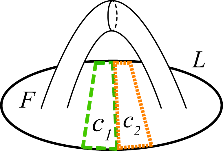
Assume that is not a -torus link. A connected collection of regions form a subsurface of with interior homeomorphic to a disk. The set of all maximal connected collections of regions forms a collection of disks with no pair of disks sharing a common arc in their boundaries.
Proof.
We first use induction to show that a connected collection of regions has interior homeomorphic to a disk. If consists of a single region, then it is a disk, since any single region is a disk. Now consider the case when consists of the union of distinct regions. The dual graph of is a finite connected graph, so we can remove some region to get a collection of regions which is also connected. By induction is a disk, and is obtained from by adding a single region sharing at least one arc with . Now consists of either one or two interior arcs. If one, then since the union of two disks intersecting along a proper arc on their boundary is a disk, it follows that the interior of is also a disk. If has two components, then is an annulus or Mobius band, properly embedded in , and coincides with either one or two components of . The boundary of a regular neighborhood in of this annulus or Mobius band is a torus, and since is alternating, the torus must be compressible in the complement of [15], and hence unknotted and the boundary of a solid torus in the complement of . Since each curve of is isotopic to a curve on this torus that intersects its meridian twice, and is not split, must be a -torus link, contradicting our hypothesis. We conclude that the connected collection of regions is homeomorphic to a disk.
A maximal connected collection of regions cannot share an interior arc with a another such region, since if it did neither would be maximal. Thus maximal connected collections are disks with no common arc in their boundaries. ∎
A consequence of Lemma 4.1 is that the isotopy class of a spanning surface does not depend at all on the location of curves.
Lemma 4.2.
The curves of and that are not of type , together with the link , determine a unique spanning surface , up to isotopy.
Proof.
By Lemma 4.1, maximal connected collections of regions form disjoint disks when is not a -torus link. The image of the surface in the complement of the disks is determined by the configuration of curves that are not curves. Two Seifert surfaces that agree in the complement of a collection of disks are isotopic, since the link is not split, and therefore has irreducible complement. Thus the isotopy class of the spanning surface is determined once the curves that are not are specified. Finally, we note that a -torus link has a unique incompressible spanning surface. ∎
5. The number of Seifert surfaces of fixed genus
In this section, we bound the number of curves in and , and the maximum length of the word associated to each curve. This in turn gives an upper bound for the number of Seifert surfaces of a fixed genus, up to isotopy. Here and further we assume that genus .
Let denote the set of curves of and that are not of type or , and the set of curves,
Lemma 5.1.
.
Proof.
By Remark 3.2, every curve in gives a contribution to the absolute value of the Euler characteristic of of at least 1/4. The Euler characteristic of is . Thus the maximal possible size of is . ∎
Lemma 5.2.
The length of the word associated to any curve in is at most .
Proof.
We consider words associated to the curves in , since all other words are of length 4. It follows from Lemma 3.1 that each word of gives a negative contribution to the Euler characteristic of . The Euler characteristic of is , and each word contributes by Lemma 3.1, where is the number of ’s, and is the number of ’s in the word. Thus the longest possible word has length . ∎
Lemma 5.3.
.
Proof.
Every curve contains two saddles. Theorem 3 of [17] gives an upper bound of for the number of saddles in a minimal complexity diagram, where is the number of boundary components of . Each curve meets two saddles and each saddle meets four curves, thus at most words are associated to the surface . So . ∎
Theorem 5.4.
For a prime non-split alternating link with crossings, the number of isotopy classes of genus- Seifert surfaces is at most .
Proof.
In each isotopy class we choose a surface that is in minimizing standard position. There are at most 8g -4 curves in by Lemma 5.1 and curves in by Lemma 5.3. We count the number of possible configurations these curves can realize, up to isotopy of the curves.
Each of the curves in has an associated word with length at most by Lemma 5.2. Consider a curve of . The link has crossings, and each crossing gives rise to two choices for the location of an adjacent to that crossing. There are edges in the link diagram, each edge having two sides, giving choices for where an interior arc meets an edge. Choosing successive sides of saddles and edges determines a curve up to isotopy. Therefore the number of isotopy classes of a curve in , each such curve having length at most is less than . For the entire collection of up to curves, the total number of isotopy classes is bounded by . Similarly, the number of configurations for curves in is bounded by . Once the curves in and are fixed, Lemma 4.2 shows that the spanning surface is determined up to isotopy. This gives an upper bound of possible isotopy classes for . ∎
Remark 5.5.
We have not used the orientability of in the arguments above, except when we replace Euler characteristic with genus. Therefore, a similar upper bound holds for the number of spanning surfaces, oriented or not, if genus is replaced by .
Remark 5.6.
The bound in Theorem 5.4 is polynomial in when the genus is fixed. Thus the number of genus ten Seifert surfaces for a link is bounded by a polynomial function of the number of crossings as varies. However for a fixed link , the number of surfaces can grow exponentially with the genus. This can be compared with the results on immersed closed surfaces in closed hyperbolic 3-manifolds [12], [14], and with similar results for closed surfaces in alternating links [8]. We note that J. Banks constructed explicit families of prime alternating knots for which the number of minimal genus Seifert surfaces grows exponentially with the genus ([1]).
Remark 5.7.
The Kakimizu complex of a link is a simplicial complex whose vertices correspond to isotopy classes of minimal genus Seifert surfaces of , and edges correspond to disjoint (up to isotopy) pairs of such surfaces ([11]). Theorem 5.4 gives an upper bound on the number of vertices in a connected component of this complex.
6. Acknowledgments
J. Hass was partially supported by NSF grant DMS-1758107. A. Thompson was partially supported by NSF grant DMS-1664587. A. Tsvietkova was partially supported by NSF grants DMS-1406588, DMS-1664425, and by Okinawa Institute of Science and Technology funding.
References
- [1] J. E. Banks, Knots with many minimal genus Seifert surfaces, https://arxiv.org/abs/1308.3218
- [2] J. R. Eisner, Knots with infinitely many minimal spanning surfaces, Trans. Amer. Math. Soc. 229 (1977), 329–349.
- [3] F. Frankl, L. Pontrjagin, Ein Knotensatz mit Anwendung auf die Dimensionstheorie, Math. Annalen. 102 (1930), no. 1, 785–789.
- [4] J. E. Greene, Alternating links and definite surfaces, with an appendix by A. Juhász and M. Lackenby, Duke Math. J. 166 (2017), no. 11, 2133–2151
- [5] W. Haken, Theorie der Normalflächen: Ein Isotopiekriterium für den Kreisknoten’, Acta Math., 105 (1961) 245–375.
- [6] J. Hass, Acylindrical surfaces in 3-manifolds, Michigan Math. J. 42 (1995), no. 2, 357–365.
- [7] J. Hass, J. C. Lagarias and N. Pippenger, The computational complexity of Knot and Link problems, Journal of the ACM, 46 (1999) 185–211.
- [8] J. Hass, A. Thompson, A. Tsvietkova, The number of surfaces of fixed genus in an alternating link diagram, Int. Math. Res. Not. (2017), no. 6, 1611–1622.
- [9] J. Hempel, 3-Manifolds, Princeton University Press.
- [10] J. Howie, A characterisation of alternating knot exteriors, Geom. Topol. 21 (2017), no. 4, 2353–2371
- [11] O. Kakimizu, Finding disjoint incompressible spanning surfaces for a link, Hiroshima Math. J. 22 (1992), no. 2, 225–236.
- [12] J. Kahn, V. Markovic, Counting essential surfaces in a closed hyperbolic three-manifold, Geom. Topol. 16 (2012), 601–624.
- [13] H. Kneser, “Geschlossene Flächen in dreidimensionalen Mannigfaltigkeiten”, Jahresbericht Math. Verein., 28 (1929) 248–260.
- [14] J. D. Masters, Counting immersed surfaces in hyperbolic 3-manifolds, Algebr. Geom. Topol. 5 (2005), 835–864.
- [15] W. W. Menasco, Closed incompressible surfaces in alternating knot and link complements, Topology 23 (1984), 37–44.
- [16] W. Menasco, Determining incompressibility of surfaces in alternating knot and link complements, Pacific J. Math. 117 (1985), no. 2, 353–370.
- [17] W. M. Menasco, M. B. Thistlethwaite, Surfaces with boundary in alternating knot exteriors, J. Reine Angew. Math. 426 (1992), 47–65.
- [18] H. Seifert, Über das Geschlecht von Knoten, Math. Annalen. 110 (1934), no. 1, 571–592.
- [19] R. Schoen, Estimates for Stable Minimal Surfaces in Three Dimensional Manifolds 103 of Ann. of Math. Studies., Princeton University Press, 1983.
- [20] W. P. Thurston, The geometry and Topology of Three-Manifolds, Electronic Version 1.1 (March 2002), http://www.msri.org/publications/books/gt3m/
Joel Hass
Department of Mathematics
University of California, Davis
One Shields Ave, Davis, CA 95616
hass@math.ucdavis.edu
Abigail Thompson
Department of Mathematics
University of California, Davis
One Shields Ave, Davis, CA 95616
thompson@math.ucdavis.edu
Anastasiia Tsvietkova
Department of Mathematics and Computer Science
Rutgers University-Newark
101 Warren Street, Newark, NJ 07102
a.tsviet@rutgers.edu