Higher angular momentum band inversions in two dimensions

We first focus on the square lattice. Since the square lattice has $C_{4}$ rotation symmetry angular momentum can be distinguished up to $l=\pm 2$. As a result, the square lattice can support models for band inversion transitions up to Chern number $C=\pm 2$. To obtain such models it is natural to choose on-site orbital degrees of freedom with relative angular momentum $\pm 2$. We thus consider $s$-wave and $d_{xy}$-wave orbitals and define $s_{\bf k}$ and $d_{\bf k}$ as the electron annihilation operators corresponding to the $s$- and $d$-wave states. (The symmetry of the higher angular momentum orbitals is shown in Fig. 2.) We write the Hamiltonian $H$ for this two-band system as

where the Hamiltonian matrix $h_{\bf k}$ may be expanded in Pauli matrices $\tau_{x,y,z}$.

As outlined in the beginning of this section, the form of $h_{\bf k}$ is determined by the symmetry requirements of a $C_{4}$ symmetric Chern insulator and symmetry of the $s$- and $d$-wave states. An elegant and simple way to derive the form of $h_{\bf k}$ is to formulate the allowed couplings in terms of lattice harmonic functions, which may be viewed as lattice analogs of spherical harmonics and describe hoppings with distinct symmetry. As an example, the (lowest order) $s$-wave harmonic $\lambda^{s}_{\bf k}$ given by

corresponds to the standard nearest neighbor hopping. Note that due to the discrete symmetry of a lattice the lattice harmonics are labeled by the finite set of point group representations (see Table 1). The two $d$-wave harmonics with $d_{x^{2}-y^{2}}$ and $d_{xy}$ symmetry are given by

and the $p$-wave harmonics are given by $(\lambda^{p_{1}}_{\bf k},\lambda^{p_{2}}_{\bf k})=(\sin k_{x},\sin k_{y})$. The symmetry properties and the point group labels of the lattice harmonics are summarized in Table 1 and are shown schematically in Fig. 2.

Using the symmetry of the orbital basis states and the lattice harmonics it is straightforward to construct a Hamiltonian $H$ which satisfies all symmetry requirements and has a gapped ground state. We write the $H$ as a sum of two parts $H_{\delta}$ and $H_{\Delta}$. Here $H_{\delta}$ describes both nearest neighbor intra-orbital hopping and an energy splitting $\varepsilon_{s}-\varepsilon_{d}$ of the $s$ and $d$ states, and $H_{\Delta}$ describes the (inter-orbital) couplings between the $s$ and $d$ states. The splitting between the $s$ and $d$ states is conveniently parametrized as $\varepsilon_{s}-\varepsilon_{d}=2t-\delta$, where $t$ is the nearest neighbor hopping parameter; $H_{\delta}$ then takes the form

The structure of $H_{\Delta}$ follows from the observation that $d^{\dagger}_{\bf k}s_{\bf k}$ transforms as a $d_{xy}$ wave. The simplest rotationally invariant but $T$- and $M$-broken coupling then takes the form

where $\Delta_{1,2}$ are both real and the relative phase is responsible for broken $T$. Combining these two terms we arrive at the form of $h_{\bf k}$ given by

where we defined $\varepsilon_{\bf k}=2t-\delta-t\lambda^{s}_{\bf k}$. The square lattice model defined by (13) is shown pictorially in Fig. 3 ($\bf A$).

It is straightforward to verify that $h_{\bf k}$ has a gapped spectrum for nonzero $(\delta,\Delta_{1},\Delta_{2})$ and supports Chern bands with $C=\pm 2$ for $4t>\delta>0$. The parameter $\delta$ can be directly identified with the band inversion parameter of Eq. (2). The spectrum of (13) is shown in Fig. 3 ($\bf B$)–($\bf D$), corresponding to the inverted regime ($\delta>0$), the critical point ($\delta=0$), and the normal regime ($\delta<0$). A more detailed analysis of Eq. (13) from the perspective of Eq. (2) will be presented below.

Next, we turn to the triangular lattice, which has sixfold rotation symmetry and allows to resolve angular momentum up to $l=\pm 3$. We introduce $s$-wave and $f$-wave states as on-site orbital degree of freedom and define the corresponding electron (annihilation) operator as

As there are two symmetry-distinct $f$ waves, we fix the symmetry by declaring that $f^{\dagger}_{\bf k}$ creates electrons in a $f_{x^{3}-3xy^{2}}$ orbital state, see Fig. 2.

To determine the form of the Hamiltonian $h_{\bf k}$ on the triangular lattice we must first specify the triangular lattice harmonics. To this end it is helpful to define the three lattice vectors ${\bf a}_{i=1,2,3}$ as

The symmetric $s$-wave harmonic then takes the form $\lambda^{s}_{\bf k}=\sum_{i=1}^{3}\cos k_{i}$, where $k_{i}={\bf k}\cdot{\bf a}_{i}$. The two lowest order symmetry-distinct $f$-wave harmonics are given by

where the latter corresponds to next-nearest neighbor coupling (the proportionality constant is chosen for convenience). The $f$ waves $f_{1}$ and $f_{2}$ are identified with $f_{x^{3}-3xy^{2}}$ and $f_{y^{3}-3yx^{2}}$, respectively. In systems with hexagonal symmetry both the $p$ waves $(\lambda^{p_{+}}_{\bf k},\lambda^{p_{-}}_{\bf k})$ and the $d$ waves $(\lambda^{d_{+}}_{\bf k},\lambda^{d_{-}}_{\bf k})$ are degenerate, i.e., they form partners of a two-dimensional representation. Expressed in the chiral basis $p_{\pm}=p_{x}\pm ip_{y}$ and $d_{\pm}=d_{x^{2}-y^{2}}\pm id_{xy}$, the triangular lattice $p$- and $d$-waves harmonics take the form

with $\omega=e^{2\pi i/3}$ and $\lambda^{-}_{\bf k}=(\lambda^{+}_{\bf k})^{*}$. Note that the $p_{x,y}$ waves $(\lambda^{p_{1}}_{\bf k},\lambda^{p_{2}}_{\bf k})$ are simply obtained via the relation $\lambda^{p_{\pm}}_{\bf k}=\lambda^{p_{1}}_{\bf k}\pm i\lambda^{p_{2}}_{\bf k}$, and similarly for the $d$ waves.

Given the triangular lattice harmonics and their symmetry properties, we directly obtain the triangular lattice analog of Eq. (13) given by

Here we have defined the difference of on-site energies $\varepsilon_{s}-\varepsilon_{f}$ as $3t-\delta$ and $\varepsilon_{\bf k}=3t-\delta-t\lambda^{s}_{\bf k}$, where $t$ denotes ordinary nearest neighbor hopping. The invariance of $h_{\bf k}$ under $C_{6}$ rotations of follows directly from the symmetry of the $f$-waves couplings. This may be seen, for instance, from Fig. 2. Since the $f$-wave harmonics are odd function of ${\bf k}$, the second term in Eq. (18) is invariant under $T$, whereas the third term breaks both $T$ and $M$. A schematic representation of the triangular lattice model of (18), in particular the inter-orbital hoppings described by $\Delta_{1,2}$, is shown in Fig. 4 ($\bf A$). For nonzero $(\delta,\Delta_{1},\Delta_{2})$ the spectrum of $h_{\bf k}$ has a full energy gap and the two non-degenerate bands are Chern bands with $C=\pm 3$ when $4t>\delta>0$. A plot of the energy bands in the inverted regime, $\delta=0.5t$, is shown in Fig. 4 ($\bf B$). Note that the gap is proportional to $\delta^{3/2}$. Below, in Sec. III.1.4, we discuss the low-energy limit of the transition as function of $\delta$ in more detail.

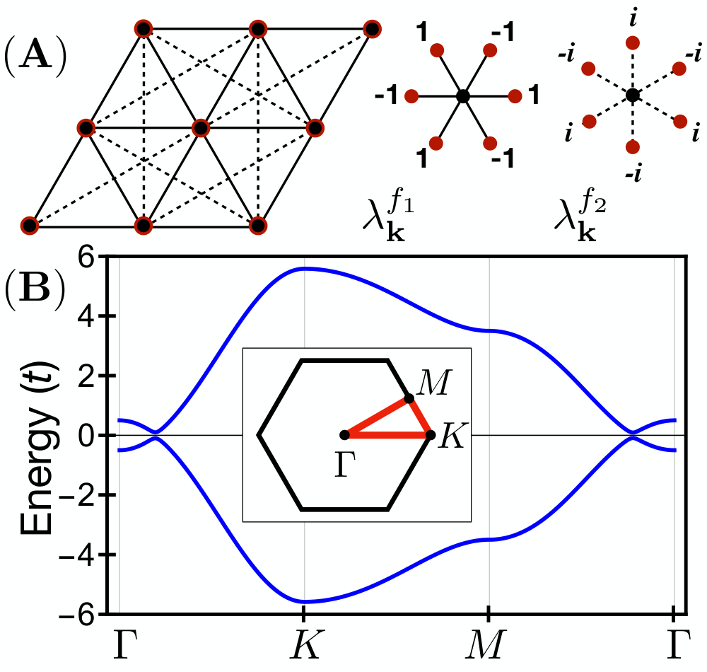
In addition to the triangular lattice model with $C=\pm 3$ bands, it is straightforward to construct a triangular lattice model with $C=\pm 2$ bands. This is achieved by considering $s$-orbital and $d$-orbital states as local degrees of freedom, and since the two $d$-wave states $(d_{x^{2}-y^{2}},d_{xy})$ are degenerate both should be included a priori. Consider the following model describing the coupling of $s$ and $d$ states, where $d_{{\bf k}1,2}$ annihilate electrons with $d_{x^{2}-y^{2},xy}$-orbital symmetry:

Once more we have defined $\varepsilon_{\bf k}=3-\lambda^{s}_{\bf k}+\delta$ and the operators $d_{{\bf k}\pm}=d_{{\bf k}1}\pm id_{{\bf k}2}$ correspond to the chiral basis of the $d$-wave states; a sum over $\alpha=1,2$ is implied. Observe that the term proportional to $\Delta$, which couples the $s$- and $d$-states, is fully invariant under rotations. Furthermore, it is invariant under $T$ and $M$. The second term, on the other hand, which is proportional to $\Omega$ and energetically splits chiral $d$-waves, breaks $T$ and $M$ symmetry. We may choose this energy scale to be positive and very large, i.e., $\Omega\gg 1$, and project out the $d_{{\bf k}-}$ states to obtain an effective model for the $s$ and $d_{+}$ states. Note that projecting out the $d_{{\bf k}-}$ states is consistent with $C_{6}$ symmetry and broken $T$ and $M$ symmetry. The reduced two-band model can the expressed in the form of (8) with $h_{\bf k}$ given by

where $\tau_{\pm}\equiv(\tau_{x}\pm i\tau_{y})/2$. This Hamiltonian describes a transition as function of $\delta$ from a trivial insulator to a Chern insulator with $C=\pm 2$ on the triangular lattice. Note that, contrary to Eq. (18) or (13), there is only one parameter $\Delta$ describing the coupling of $s$- and $d$-states, which is due to $C_{6}$ symmetry.

Clearly, by simply making the replacement $d\to p$ in Eq. (19) this construction directly applies to states with $p$-wave symmetry, in which case one obtains a $C=\pm 1$ Chern insulator model. Furthermore, the $p$-wave model is easily generalized to the square lattice using the square lattice harmonics [40], leading to the spinless (and lattice-regularized) Bernevig-Hughes-Zhang (BHZ) model [2].

Up to this point, we have considered onsite orbital degrees of freedom with nonzero angular momentum. This might suggest that the models introduced here require higher angular momentum atomic-like states (see Fig. 2) at sites of the crystal lattice. In fact, our construction is more general, and also applies to cases for which effective higher angular momentum states arise as a result of the structure of the unit cell. More specifically, in crystal lattices with a nontrivial unit cell, i.e., a unit cell containing multiple atoms which map to each other under symmetry operations, one can form symmetrized states within the unit cell. These symmetrized states transform nontrivially under the symmetry group in a way that is equivalent to nonzero angular momentum states. Therefore, the orbital states shown in Fig. 2 should be understood in a more general sense as states of a specific symmetry type, rather than atomic orbitals.

To illustrate this with an example, we now consider a simple honeycomb lattice model for spinless electrons. The honeycomb lattice, which has a triangular Bravais lattice, consists of two (triangular) sublattices, the $A$ and $B$ sublattice, and we define the corresponding electron operators as $a_{{\bf k}}$ and $b_{\bf k}$. As before, we collect these in a spinor

The Hamiltonian $H$ is defined as $H=\sum_{\bf k}\varphi^{\dagger}_{\bf k}h_{\bf k}\varphi_{\bf k}$ with $h_{\bf k}$ given by

Here $\phi_{\bf k}$ is a honeycomb lattice harmonic describing nearest neighbor hopping and is defined as $\phi_{\bf k}=\sum_{i}e^{i{\bf k}\cdot{\bf d}_{i}}$, where ${\bf d}_{i=1,2,3}$ are the three nearest neighbor bond vectors ${\bf d}_{i=1,2,3}=(\sin\theta_{i},\cos\theta_{i})^{T}/\sqrt{3}$. [The angles $\theta_{i=1,2,3}$ are the same as in Eq. (15).] Furthermore, the honeycomb lattice harmonic $\phi^{\prime}_{\bf k}=\sum_{i}e^{-2i{\bf k}\cdot{\bf d}_{i}}$ describes third nearest neighbor hopping across a hexagon and the final term proportional to $t_{H}$ is the Haldane term [16], with $\lambda^{f_{1}}_{\bf k}$ defined in Eq. (16). The three hoppings are shown in Fig. 5 ($\bf B$), where arrows indicate $T$-breaking imaginary hopping.

To see how Eqs. (21) and (22) give rise to states which have the symmetry of higher angular momentum orbitals consider the Hamiltonian at ${\bf k}=0$. The Hamiltonian takes the form $h_{{\bf k}=0}=(t-t^{\prime})\tau_{x}$, which implies that the eigenstates are the even and odd linear combinations $a_{{\bf k}=0}\pm b_{{\bf k}=0}$. Clearly, the odd linear combination is odd under all symmetries of the honeycomb lattice which exchange the sublattices and therefore the eigenstates at ${\bf k}=0$ transform as $s$ and $f$ waves. Now, if we redefine $t^{\prime}=t-\delta$, then $\delta$ parametrizes a band inversion transition of two bands with relative angular momentum $l=3$ at ${\bf k}=0$. As a result, Eq. (22) falls in the class of models of which the low-energy description is captures by Eq. (2).

It is easy to recognize that the Hamiltonian of Eq. (22) can be viewed as a simple generalization of the Haldane model introduced in Ref. 16. In the context of the Haldane model the band inversion transition described by Eq. (22) can be understood as follows. First, we take $t^{\prime}=0$ but choose $t_{H}$ nonzero; this is the Haldane model and describes a Chern insulator with $C=\pm 1$ bands. Now we turn on and increase $t^{\prime}$ (which we take positive). As long as the gap stays open the ground state is a Chern insulator with $C=\pm 1$ bands. At $t^{\prime}=t$ the gap closes and reopens for $t^{\prime}>t$. Since this transition is an angular momentum $l=\pm 3$ transition the Chern numbers must have changed by $\pm 3$ and indeed we find the resulting bands to have Chern number $C=\mp 2$. (Note that the sign of $C$ is determined by the sign of $t_{H}$.) As a result, neither side of the transition corresponds to the trivial insulator. A plot of the bands for $t^{\prime}>t$ is shown in Fig. 5 ($\bf A$). Note that a large $t_{H}$ leads to a large separation of bands at $K$, which can be viewed as a large mass for the graphene Dirac points.

In the models presented above, in particular the square and triangular lattice models, we have made use only of the lowest order lattice harmonics, i.e., we included the nearest (or at most next-nearest) neighbor couplings. As our considerations have shown, for the purpose of constructing models with a low-energy description given by Eqs. (2) and (3) this is sufficient. In general, one may include higher order lattice harmonics in the same symmetry class without affecting the essential physics described by the model.

We now turn to a more detailed analysis of Eqs. (13) and (18) from the viewpoint of higher angular momentum band inversion transitions introduced in Sec. II. We begin by expanding the coupling terms of the former, which should be identified with $\Delta_{\bf k}$ of Eq. (3), to lowest order in ${\bf k}$ and find for $m=2,3$

where $m=2$ and $m=3$ correspond to Eqs. (13) and (18), respectively. The fact that both $k^{m}_{+}$ and $k^{m}_{-}$ appear is due to discrete crystal symmetry; the form of Eq. (3) is only recovered at a fine-tuned point when $\Delta_{1}=\Delta_{2}$. The dominant term is determined by the relative magnitude of $|\Delta_{1}+\Delta_{2}|$ and $|\Delta_{1}-\Delta_{2}|$, which also determines the Chern number in the band inverted regime. By changing one of the two parameters $\Delta_{1,2}$ while keeping the other fixed, the system undergoes a transition from a Chern number $C=\pm m$ phase to a Chern number $C=\mp m$ phase. This transition occurs via a mass inversion at $2m$ Dirac points located on the electron-hole Fermi surface defined by $k_{F}$ (see Sec. II). Note that this is consistent with the fact that in a $C_{n}$ symmetric system the Chern number can only be determined from the rotation eigenvalues mod $n$ [15]; here we have $2m=n$ for $m=2,3$ and $n=4,6$.

Now, let us address the question whether (13) and (18) represent the most general form a Hamiltonian consistent with $C_{4}$ or $C_{6}$ rotation symmetry. That is to say, we ask whether there might be additional terms which can be added to (13) and (18) while preserving its generic structure. In the case of $C_{4}$ symmetry, we can reconsider Eq. (12) and observe that in general $\Delta_{1}$ and $\Delta_{2}$ can be complex. This more general Hamiltonian is still symmetric under $C_{4}$ rotations and translates into an additional term in Eq. (13) given by $\Delta^{\prime}_{1}\lambda^{d_{1}}_{\bf k}\tau_{x}+\Delta^{\prime}_{2}\lambda^{d_{2}}_{\bf k}\tau_{y}$. Expanding this full $C_{4}$-symmetric Hamiltonian, with four real parameters describing the coupling, in small momenta ${\bf k}$ one finds

with $\tilde{\Delta}_{\pm}$ given by

From this we conclude that a full account of the symmetry-allowed couplings leads a low-energy Hamiltonian of the form Eqs. (2) and (3) with $\Delta_{\bf k}$ given by (24) in terms of $\tilde{\Delta}_{\pm}$. Only the magnitudes $|\tilde{\Delta}_{\pm}|$ are important for the topological classification in the inverted regime ($\delta>0$). Clearly, this conclusion holds equally for the case $m=3$ and $C_{6}$ symmetry; in particular, Eq. (25) is still valid.

To begin, consider the low-energy description of the square and triangular lattice models of Eqs. (13) and (18). In the analysis that follows we particularize to these models for illustrative purposes, without loss of generality. Consider furthermore the special case $\Delta_{1}=\Delta_{2}\equiv\Delta$; according to Eq. (23), for small momenta ${\bf k}$ this implies $\Delta_{\bf k}\sim\Delta_{m}(k_{x}-ik_{y})^{m}$ with $m=2,3$. Based on Eq. (25), we promote $\Delta_{m}$ to a complex number with arbitrary phase. In addition, in the small momentum limit one has $\varepsilon_{\bf k}\simeq{\bf k}^{2}/2-\delta$. As discussed, the form of $\Delta_{\bf k}$ (i.e., an eigenstate of $L_{z}$ with angular momentum $l=-m$) is determined by the rotational symmetry of the system. Importantly, the formation of excitons, i.e., excitonic pairing, alters the form of $\Delta_{\bf k}$ and breaks rotational symmetry. Specifically, in a mean field description of excitonic pairing $\Delta_{\bf k}$ becomes

where $m=2,3$ and $\Delta_{0}$ represents the formation of excitons. We observe that $\Delta_{0}$ is an angular momentum $l=0$ coupling of conduction and valence band, and since (30) is a superposition of terms with different angular momentum, rotational symmetry is broken. In the low-energy continuum limit the $l=0$ angular momentum term breaks the emergent continuous rotation symmetry and lowers the symmetry to $\mathbb{Z}_{m}$. In particular, $\Delta_{0}$ transforms as $\Delta_{0}\to e^{-im\theta}\Delta_{0}$ under rotations by an angle $\theta$. This establishes a link between the phase of $\Delta_{0}$ and rotation symmetry breaking, which is analogous to the link between the superconducting phase and $U(1)$ charge conjugation.

On the lattice, in the case $m=2$ the fourfold rotation $C_{4}$ is reduced to $C_{2}$; in the case $m=3$ the rotational symmetry is lowered from $C_{6}$ to $C_{3}$. In both cases, $m=2$ and $m=3$, the form of (30) can be derived from a lattice model mean field Hamiltonian given by $h_{\bf k}\to h_{\bf k}+\Delta_{0}\tau_{+}+\Delta^{*}_{0}\tau_{-}$.

To examine the implications of (30), in particular the excitonic term, it is useful to invoke the connection to the problem of pairing states. In the context of pairing states, $\Delta_{0}$ can be interpreted as an $s$-wave pairing. Assuming one is in the band inverted regime, this implies a transition as function of the strength of $\Delta_{0}$, from a Chern insulating phase to a trivial insulator phase. This implication follows from the fact that $s$-wave pairing is topologically trivial. The transition occurs when $|\Delta_{0}|=|\Delta_{m}|k^{m}_{F}=|\Delta_{m}|(2\delta)^{m/2}$, where $k_{F}$ is a momentum defined by the condition $\varepsilon_{\bf k}=0$ (see Sec. II). At the transition the system is gapless, with three ($m=3$) or two ($m=2$) Dirac points located in a circle in momentum space with radius $k_{F}$. Thus, the transition is marked by three (or two, in the case of $m=2$) Dirac fermion mass inversions, which is consistent with the total change in the Chern number. This is shown schematically in Fig. 6 for the case $m=3$. Note that the location of the Dirac points depends on the phase of $\Delta_{0}$: assuming $\Delta_{0}=|\Delta_{0}|e^{i\theta_{0}}$ and $\Delta_{m}$ real but negative, the Dirac points are located at angles $\theta_{0}/m+j2\pi/m$ with $j=0,1,2$.

Having discussed the qualitative features of the excitonic mean field theory, we now turn to a more quantitative analysis. To this end, we take the triangular lattice model of Eq. (18) (the analysis is similar for the $m=2$ square lattice model), in which we set $\Delta_{1}=\Delta_{2}\equiv\Delta_{m=3}$, and add an onsite Hubbard repulsion of the form $H_{U}=U\sum_{j}n_{js}n_{jf}$, where $n_{s,f}$ are the density operators of the $s$ and $f$ orbitals and the sum is over sites. In momentum space the Hubbard repulsion takes the form

where $N$ is the system size (i.e., total number of sites). By performing a mean field decoupling of (31) in the excitonic channel (see Appendix B for details) one obtains a self-consistency condition for the excitonic order parameter $\Delta_{0}$ given by

Here $\varphi_{\bf k}$ are the fermion operators defined in Eq. (14). At zero temperature Eq. (32) defines the stationary point of the free energy density

where $\Sigma_{\bf k}$ is defined as $\Sigma_{\bf k}=\Delta_{0}+\Delta_{\bf k}$ with $\Delta_{\bf k}=\Delta_{3}(i\lambda^{f_{1}}_{\bf k}+\lambda^{f_{2}}_{\bf k})$.

Solving these equations at zero temperature, we obtain a phase diagram of excitonic pairing as function of the interaction strength $U$ and the band inversion parameter $\delta$. The results are presented in Fig. 7, which we now discuss. We first focus on the case $\delta=0$. In this case, the non-interacting systems is right at the topological transition and is gapless, with two quadratically dispersing bands touching at ${\bf k}=0$. As a consequence of the non-vanishing density of states at the gapless point, the susceptibility is divergent and one expects a rotation symmetry broken state with nonzero $\Delta_{0}$ at infinitesimal $U$. More precisely, one expects $\Delta_{0}\sim\exp(-1/\alpha U)$, where $\alpha$ is a constant reflecting the density of states [24]. This is confirmed in Fig. 7 ($\bf A$), where we show $\ln\Delta_{0}$ as function of $-1/U$ for the case $\delta=0$. (In all calculations we choose $\Delta_{3}=0.5t$.)

We then proceed to the case $\delta\neq 0$. For nonzero $\delta$, when the non-interacting system given by $h_{\bf k}$ in Eq. (18) is gapped, one expects a transition to the rotation symmetry broken state at finite interaction strength $U_{c}$. The critical interaction strength as function of $\delta$ defines the phase boundary which separates the rotation symmetric phase from the rotation symmetry broken phase with nonzero excitonic pairing. Since the inverted regime ($\delta>0$) and the uninverted regime ($\delta<0$) have different dispersion, as is clear from Fig. 1 ($\bf A$) and ($\bf C$), the critical strength $U_{c}$ is expected to be smaller in the inverted regime. We find that the transition to the symmetry broken phase is a second order transition in mean field theory, which implies that a closed form expression for $U_{c}$ can be obtained by expanding $F$ of Eq. (68) in powers of $\Delta_{0}$. Such Landau-type expansion can only have even powers of $\Delta_{0}$ and is valid in the vicinity of the transition when $\Delta_{0}$ is small; specifically, one has up to fourth order

Then, $U_{c}$ is defined by the condition that the coefficient of the quadratic term vanishes and we find

where $E_{\bf k}$ defined in Eq. (68) is evaluated at $\Delta_{0}=0$. Figure 7 ($\bf B$) shows the $U$–$\delta$ phase diagram obtained by evaluating $U_{c}$ as function of $\delta$. As expected, $U_{c}$ is smaller in the inverted regime (blue curve) compared to the uninverted regime (red curve).

As discussed above in Sec. IV.1.1, in the inverted regime defined by $\delta>0$ one expects a second transition as the interaction strength increases. This second transition is a topological phase transition described by three Dirac fermions and occurs when $|\Delta_{0}|\sim|\Delta_{{\bf k}=k_{F}}|$. One may thus identify a second $U^{\prime}_{c}$ associated with the topological phase transition and it is then natural to ask how $U^{\prime}_{c}$ differs from $U_{c}$. To get an understanding we employ the Landau theory of Eq. (34) and solve for $\Delta_{0}$. Minimization directly yields $|\Delta_{0}|=\sqrt{(c_{2}-U^{-1})/2c_{4}}$. Within this approach the value of $U^{\prime}_{c}$ is determined by setting this result equal to the value of $\Delta_{0}$ at which which the topological transition occurs. Defining the latter as $\tilde{\Delta}_{0}$, we find

We have verified that this estimate based on (34) is in good agreement with the numerically exact result. Since $(2c_{4}U_{c}\tilde{\Delta}^{2}_{0})^{-1}\gg 1$, Eq. (36) implies that the transitions, i.e., the symmetry breaking transition and the topological transition, are in close proximity. This is indicated by the dashed line in Fig. 7 ($\bf B$). To understand why $(U^{\prime}_{c}-U_{c})/U_{c}$ is small, it is helpful to consider the continuum description discussed in Sec. IV.1.1, which is valid for small $\delta$. In this case one has $\tilde{\Delta}^{2}_{0}\sim\delta^{3}$ and $c_{4}\sim\delta^{-2}$, from which one finds $(U^{\prime}_{c}-U_{c})/U_{c}\sim\delta/\ln\delta$. Note that in case of the square lattice one finds $(U^{\prime}_{c}-U_{c})/U_{c}\sim 1/\ln\delta$.

The close proximity of the two transitions is an interesting aspect of higher angular momentum band inversions. The fate of these two transitions in an interacting theory beyond mean field will be an interesting question to address. Such theory should be formulated in terms of three flavors of Dirac fermions coupled to a fluctuating phase of the excitonic order parameter $\Delta_{0}$, as suggested by Fig. 6.

References

- [1] N. Read and D. Green, Phys. Rev. B 61, 10267 (2000).
- [2] B. A. Bernevig, T. L. Hughes, and S.-C. Zhang, Science 314, 1757 (2006).
- [3] L. Fu and C. L. Kane, Phys. Rev. B 76, 045302 (2007).
- [4] M. Z. Hasan and C. L. Kane, Rev. Mod. Phys. 82, 3045 (2010).
- [5] X.-L. Qi and S.-C. Zhang, Rev. Mod. Phys. 83, 1057 (2011).
- [6] A. P. Schnyder, S. Ryu, A. Furusaki, and A. W. W. Ludwig, Phys. Rev. B 78, 195125 (2008).
- [7] C.-K. Chiu, J. C. Y. Teo, A. P. Schnyder, and S. Ryu, Rev. Mod. Phys. 88, 035005 (2016).
- [8] A. W. W. Ludwig, M. P. A. Fisher, R. Shankar, and G. Grinstein, Phys. Rev. B 50, 7526 (1994).
- [9] L. Fu, C. L. Kane, and E. J. Mele, Phys. Rev. Lett. 98, 106803 (2007).
- [10] C. Fang, M. J. Gilbert, X. Dai, and B. A. Bernevig, Phys. Rev. Lett. 108, 266802 (2012a).
- [11] B. Bradlyn, L. Elcoro, J. Cano, M. G. Vergniory, Z. Wang, C. Felser, M. I. Aroyo, and B. A. Bernevig, Nature 547, 298 (2017).
- [12] H. C. Po, A. Vishwanath, and H. Watanabe, Nat. Commun. 8, 50 (2017).
- [13] J. Kruthoff, J. de Boer, J. van Wezel, C. L. Kane, and R.-J. Slager, Phys. Rev. X 7, 041069 (2017).
- [14] T. L. Hughes, E. Prodan, and B. A. Bernevig, Phys. Rev. B 83, 245132 (2011).
- [15] C. Fang, M. J. Gilbert, and B. A. Bernevig, Phys. Rev. B 86, 115112 (2012b).
- [16] F. D. M. Haldane, Phys. Rev. Lett. 61, 2015 (1988).
- [17] D. J. Thouless, M. Kohmoto, M. P. Nightingale, and M. den Nijs, Phys. Rev. Lett. 49, 405 (1982).
- [18] K. v. Klitzing, G. Dorda, and M. Pepper, Phys. Rev. Lett. 45, 494 (1980).
- [19] N. Regnault and B. A. Bernevig, Phys. Rev. X 1, 021014 (2011).
- [20] S. A. Parameswaran, R. Roy, and S. L. Sondhi, Comptes Rendus Physique 14, 816 (2013).
- [21] T. Neupert, C. Chamon, T. Iadecola, L. H. Santos, and C. Mudry, Physica Scripta 2015, 014005 (2015).
- [22] Z. Liu and E. J. Bergholtz, Int. J. Mod. Phys. B 27, 1330017 (2013).
- [23] X. Liu, Z. Wang, X. C. Xie, and Y. Yu, Phys. Rev. B 83, 125105 (2011).
- [24] K. Sun, H. Yao, E. Fradkin, and S. A. Kivelson, Phys. Rev. Lett. 103, 046811 (2009).
- [25] F. Zhang, H. Min, M. Polini, and A. H. MacDonald, Phys. Rev. B 81, 041402 (2010).
- [26] O. Vafek and K. Yang, Phys. Rev. B 81, 041401 (2010).
- [27] R. Nandkishore and L. Levitov, Phys. Rev. B 82, 115124 (2010).
- [28] S. Uebelacker and C. Honerkamp, Phys. Rev. B 84, 205122 (2011).
- [29] J. M. Murray and O. Vafek, Phys. Rev. B 89, 201110 (2014).
- [30] B. Dóra, I. F. Herbut, and R. Moessner, Phys. Rev. B 90, 045310 (2014).
- [31] Y. Hu, J. W. F. Venderbos, and C. L. Kane, Phys. Rev. Lett. 121, 126601 (2018).
- [32] D. Jérome, T. M. Rice, and W. Kohn, Phys. Rev. 158, 462 (1967).
- [33] F. Wang and Y. Ran, Phys. Rev. B 84, 241103 (2011).
- [34] Y.-F. Wang, H. Yao, C.-D. Gong, and D. N. Sheng, Phys. Rev. B 86, 201101 (2012).
- [35] S. Yang, Z.-C. Gu, K. Sun, and S. Das Sarma, Phys. Rev. B 86, 241112 (2012).
- [36] M. Trescher and E. J. Bergholtz, Phys. Rev. B 86, 241111 (2012).
- [37] S. Kourtis, Phys. Rev. B 97, 085108 (2018).
- [38] C. Nayak, Phys. Rev. B 62, 4880 (2000).
- [39] F. D. M. Haldane, Phys. Rev. Lett. 93, 206602 (2004).
- [40] N. Nagaosa, J. Sinova, S. Onoda, A. H. MacDonald, and N. P. Ong, Rev. Mod. Phys. 82, 1539 (2010).
- [41] J. Dubail and N. Read, Phys. Rev. B 92, 205307 (2015).
- [42] M. Barkeshli and X.-L. Qi, Phys. Rev. X 2, 031013 (2012).
- [43] B. A. Bernevig and S.-C. Zhang, Phys. Rev. Lett. 96, 106802 (2006).
- [44] M. Levin and A. Stern, Phys. Rev. Lett. 103, 196803 (2009).
- [45] A. Karch, J. Maciejko, and T. Takayanagi, Phys. Rev. D 82, 126003 (2010).
- [46] Y.-M. Lu and Y. Ran, Phys. Rev. B 85, 165134 (2012).
- [47] A. Chan, T. L. Hughes, S. Ryu, and E. Fradkin, Phys. Rev. B 87, 085132 (2013).
- [48] J. Maciejko and G. A. Fiete, Nature Physics 11, 385 (2015).
- [49] T. Neupert, L. Santos, S. Ryu, C. Chamon, and C. Mudry, Phys. Rev. B 84, 165107 (2011).
- [50] C. Repellin, B. A. Bernevig, and N. Regnault, Phys. Rev. B 90, 245401 (2014).
- [51] C. L. Kane and E. J. Mele, Phys. Rev. Lett. 95, 226801 (2005).
- [52] H. Shapourian and T. L. Hughes, Phys. Rev. B 93, 075108 (2016).
- [53] B.-J. Yang and N. Nagaosa, Nat. Commun. 5, 4898 (2014).
Appendix A Ground state of Hamiltonian (2)
The Hamiltonian of Eq. (2) is diagonalized with the help of the unitary matrix , which contains the eigenvectors as its columns, and one has