Electrodynamics of binary neutron star mergers
Abstract
We consider electromagnetic interaction and precursor emission of merging neutron stars. Orbital motion of the magnetized neutron star may revive pair production within the common magnetosphere years before the merger, igniting pulsar-like magnetospheric dynamics. We identify two basic scenarios: (i) only one star is magnetized (1M-DNS scenario) and (ii) both stars are magnetized (2M-DNS scenario). Inductively created electric fields can have component along the total magnetic field (gaps) and/or the electric field may exceed the value of the local magnetic field. The key to the detection is orbital modulation of the emission. If only one star is magnetized (1M-DNS scenario) the emission is likely to be produced along the direction of the magnetic field at the location of the secondary; then, if the magnetic axis is misaligned with the orbital spin, this direction is modulated on the orbital period. For the 2M-DNS scenario, the structure of the common magnetosphere of the non-rotating neutron stars is complicated, with gaps, but no regions; there is strong orbital variations for the case of misaligned magnetic moments. For the same parameters of neutron stars the 2M-DNS scenario has intrinsically higher potential than the 1M-DNS one. The overall powers are not very high, erg s-1; the best chance to detect electromagnetic precursors to the merging neutron stars is if the interaction of their magnetospheres leads to the production of pulsar-like coherent radio emission modulated at the orbital period, with luminosity of up to Jankys at the time the merger.
Keywords:
Physical Data and Processes: acceleration of particles, magnetic fields, plasmas; Stars: gamma-ray burst: generalI Introduction: expected precursors to DNS mergers
The detection of gravitational waves associated with a GRB [1] identifies merger of neutron stars as the central engine. It is highly desirable to detect any possible precursor to the main event. At the time of the merger the electromagnetic interaction of the neutron stars can be considered as interaction of magnetized dipole(s), §II. [11] [13, see also] argued that magnetospheric interaction during double neutron star (DNS) merger can lead to the production of electromagnetic radiation. The underlying mechanism advocated in those works is a creation of inductive electric field due to the relative motion of one NS, assumed to be unmagnetized, in the magnetic field of the companion [9, 17]. Below we call it the 1M-DNS case, §III.
Typically simulations of the DNS merger with magnetic field is done within the MHD approximation [29, 28, 31, 30, 2, e.g.]. These simulations are well suited to understanding the overall structure of the interacting magnetospheres. But they do no capture the dissipative/acceleration process. In MHD (even with resistivity) the formation of gaps is prohibited. Thus, such simulations will miss the effects we discuss below - formation of gaps and dissipative regions with . We develop a complimentary electromagnetic model of interacting magnetospheres, based on the pulsar magnetosphere model of [9].
We expect that gaps forming in the magnetosphere of interacting neutron stars are not sustainable for a long time: if they create pairs the resulting charge separation screens the parallel electric field, often in a non-stationary way [14, 34]. As a result, the magnetospheric structure would generally evolve towards ideal MHD limit (without parallel component of the electric field), with a network of current sheets. Simulations of [29] do show strong magnetospheric interaction and formation of current sheets. Particles accelerated in reconnection events at these current sheets [18, e.g.] can also produce unstable distribution and coherent radio emission.
In this paper we first consider the structure of the common magnetosphere within the 1M-DNS model and then point out that the interaction of the magnetospheres of the two magnetized neutron stars - 2M-DNS scenario- will produce more powerful emission, §IV. Most importantly, in both cases we expect orbital-dependent emission pattern, that is a key to a possible future detection.
II Orbital resurrection of the rotationally dead
A neutron star after a time since birth will have a spin period [9]
| (1) |
where the surface magnetic field G is assumed, is time in gigayears; g cm2 is the moment of inertia, km is neutron star radius. Thus in a giga-year a star spins down to seconds.
The electric potential due to pulsar spin is [9]
| (2) |
Typically, vacuum breakdown occurs at GeV [7, 6, 12, 34]. Thus the merging neutron star are likely to be dead pulsars, with no pair production within their magnetospheres. [33, There is an apparent exception to this, ]
At the orbital separation the time to merger is [26]
| (3) |
The light cylinder becomes smaller that the orbital size at time
| (4) |
Thus for a few hundred million years the neutron stars are within each other’s magnetosphere, so that their interaction can be considered as an interaction of either a vacuum dipole with a highly conducting sphere (if only one star is magnetized) or two vacuum dipoles. At this point stars are separated by . (Also, the light cylinder for the orbital motion when stars are separated by is located at
| (5) |
This is much larger that the size of the orbit until the final merger.)
As the stars spiral in, the magnetospheres can be revived due to relative motion of the magnet(s). On basic grounds [4, 15], if a system has typical magnetic field B, internal velocity and typical size , the electric potential and electromagnetic luminosity can be estimated as
| (6) |
In this paper we discuss two cases that both employ relations (6), but in somewhat different regime: Single-magnetized DNS (1M-DNS) and Double-magnetized DNS (2M-DNS) mergers. The case of 1M-DNS is akin to a conductor moving in magnetic field - there is then an induced electric field, mostly close to the conductor’s/neutron star’s surface, that induces a la Goldreich-Julian surface charges, that create parallel electric field, that leads to particle acceleration. In addition - this is different from the pulsar magnetosphere case - regions with can be created. Like in case of pulsars, regions with and will lead to particle acceleration, pair production, and shortening of the acceleration electric field, most likely in a non-stationary way [14].
The case of 2M-DNS involves interacting relativistic magnetospheres - here the stars play a role of the point dipoles that produce electromagnetic fields in their surrounding. Those electromagnetic fields can form gaps and/or reconnecting current sheets, leading to energization, acceleration of particles, and production of non-thermal and possibly coherent radio emission.
The power and the available potential in both cases of 1M-DNS and 2M-DNS scenarios can be estimated using (6) with typical magnetic field due to a dipole at the distance of orbital separation and typical radius in case 1M-DNS (Eq. (7)) and in the case 2M-DNS (Eq. (23).
Typically, there is enough potential (see Eqns. (7) and (23) ) to start pair production at times before merger seconds, years. At that moment the stars are separated by cm. Starting this moment we may expect some electromagnetic signal from the system.
As we discuss below, most of the common magnetosphere remains open, so that we do not expect large stationary regions filled with plasma, like in the case of pulsar’s closed field lines [9]. Also, pair production is likely to be intermittent. Thus, a vacuum approximation is expected to be a reasonable approximation.
Let us consider the electromagnetic structure of two interacting vacuum DNS magnetospheres. Following of the classic work of [9], we will find that orbiting neutron stars create electric potentials along the combined electric fields. This serves as a first-order approximation to the expected nearly ideal plasma, that at the same time has special accelerations regions with .
Let us next discuss cases 1M-DNS and 2M-DNS in detail.
III Interacting DNS magnetospheres: 1M-DNS case
If only one star is magnetized, we are dealing with a metal sphere (second neutron star) moving through the magnetic field of the primary. This was the case originally considered by [11]. Below in this section we provide a more detailed description of the resulting interaction.
III.1 1M-DNS: estimates of power
If a neutron star is moving in the field of a primaries’ dipolar magnetic field at orbital separation , the induced potential and the corresponding powers are [11, 16]
| (7) |
where in the last relations the time to merger is measured in seconds. (Index indicates here that the interaction is between single magnetized neutron star and unmagnetized one.)
III.2 1M-DNS - internal structure of the magnetosphere
Consider a highly conducting unmagnetized neutron star moving through the magnetic field of the companion. The expected parallel electric field that would develop in the system will be largest near the surface of the companion (unmagnetized) neutron star. Hence, for simplicity we approximate the dipolar magnetic field of the primary at the location of the secondary as a straight vertical field. This is a good approximation if the sizes of the stars are much smaller than the orbit.
The neutron star is highly conducting, and can be approximated as a conducting metal sphere, so that the magnetic field does not penetrate, Fig. (1).
The induced field is
| (8) |
while the total magnetic field is
| (9) |
The conducting sphere is sliding through the magnetic field with the relative velocity
| (10) |
(here is a semi-major axis). As a result magnetic field in the observer frame is time-dependent: there is non-zero , which would produce electric field. The resulting electric field will generally have a component parallel to the magnetic field.
III.3 1M-DNS - motion of the secondary in the magnetic equatorial plane of the primary
let us first consider the case when the secondary unmagnetized star is moving perpendicular to the magnetic field lines. In Eq. (9) make a transformation to the observer frame by writing . Time derivative of (9) (evaluated at arbitrary ) is
| (11) |
(in coordinates. This equals minus the curl of the induced electric field. We find a vacuum electric field with
| (12) |
(alternatively, we could do a Lorentz boost of the induced magnetic field (8), giving the same result).
The induced field (12) has a component normal to the surface of the NS, that will produce surface charge density
| (13) |
The surface charge will produce an electric field
| (14) |
The total field outside is then
| (15) |
The total magnetic and the electric fields (Eqns. (9) and (15)) have two important properties. They have non-zero first electromagnetic invariant and the second invariant can change sign.
The parallel component of the electric field equals
| (16) |
Fig. 2 shows that there are regions of non-zero parallel electric field, peaking in value close to the neutron star surface. If plasma is generated in these regions, the outflows will be directed mostly along the external magnetic field, passing close to the poles.
The parallel electric field is maximal in the plane (). At each the maximal values of is reached at . At this corresponds to , where the total magnetic field is zero.
The invariant equals
| (17) |
It becomes negative within a dome-like structure near the poles. On the surface of the neutron star it is within a region
| (18) |
(for each value of Eq. (18) gives the value of so that for smaller (closer to the pole) we have , see Fig. 3). Note that even in the plane, where the electric field is zero, the magnetic field is also zero, so that the the second invariant remains negative close to the poles. At the poles, , on the surface ; the region extends to .

It is expected that both the conditions and will lead to particle acceleration. This might create conditions favorable for the generation of coherent radio emission. Without a particular global model of particle acceleration we cannot predict in detail the expected radio signal. Both the region and the region with the largest are concentrated near the pole, so that in the case of motion in the equatorial plane, no variation is expected.
The above results can be compared with the case of a black hole moving through straight magnetic field [27, 17]. In that case two dual jets are generated. As Fig. 2 demonstrates, in the case of moving metal sphere the configuration looks similar: there are four regions with high parallel electric field.
III.4 1M-DNS - oblique motion of the secondary
Above, in §III.3 we considered the motion of the secondary unmagnetized neutron star in constant magnetic field, a case applicable to when the magnetic moment of the primary is along the orbital spin. Next we generalize it to the oblique orbits of the secondary (inclined magnetic moment of the primary).
In the case of the oblique motion (not orthogonal to the spin) we can separate the motion along and across the magnetic field. For the part of motion along the external magnetic field, we find
| (19) |
Thus, this does not create a component of electric field along the magnetic field. Also, the second electromagnetic invariant
| (20) |
is always positive.
Thus what counts for the producing emission regions ( or ) is the component of the velocity perpendicular to the magnetic field. Since the primary is assumed non-rotating, only the component of the velocity perpendicular to the magnetic moment of the primary is of importance. As we argued above, the emission is likely to be produced along the magnetic field at the location of the secondary.
Consider a dipole of the primary inclined by the angle with respect to orbit normal, located at the origin, . The secondary at time is located at (in Cartesian coordinates , where is the orbital frequency. At the location of the secondary, the direction of the primary’s magnetic field is
| (21) |
in coordinates. The direction of emission varies on the orbital time scale. Thus, if emission is generated near the secondary along the local direction of the magnetic field of the primary we expect modulation of the direction on orbital time scale.
IV Interacting DNS magnetospheres: 2M-DNS case
IV.1 2M-DNS - general notes
Next we study the interaction of two dipoles that are moving with respect to each other with the (Keplerian) velocity . We can identify 4 basic geometries: (i-a) magnetic moments aligned with the orbital spin axis; (i-b) magnetic moments anti-aligned with the orbital spin axis; (ii-a) one magnetic moment is aligned with the orbital spin axis and another is along the line connecting the two neutron stars; (ii-b) one magnetic moment is aligned with the orbital spin axis and another is orthogonal both to the orbital axis and the line connecting the two neutron stars. Surely, there more complicated structures when both magnetic moments are misaligned, but these four, we think, cover the basics.
Qualitatively, cases i-a and i-b produce nearly time independent signals and are less of interest (in this case the procedure described below implies that the maximal emission is produced along the -axis, though at different orbital phases the line of sight does pass through different regions). Cases ii-a and ii-b are dynamically related - a system of neutron stars where one neutron star is aligned with the orbital spin and the spin of the order is in the orbital plane will periodically evolve from ii-a to ii-b. As we demonstrate below, this will lead to considerably different magnetospheric structures and possibly time-dependent radiative signatures.
Consider two neutron stars of same masses and producing in the surrounding space magnetic fields and . Assume that the neutron stars are non-rotating - typical merger times are much longer than the typical spin-down times and orbital synchronization is not important [3]. In the center of mass the star 1 is moving with velocity and star 2 is moving with velocity . Neglecting relativistic effects, they create the total magnetic field and the electric field . This total electric field has a component parallel to the total magnetic field:
| (22) |
which is generally non-zero. Thus, regions of non-zero parallel electric field will be created within the interacting magnetospheres.
IV.2 2M-DNS - estimates of power
In this paper we point out that magnetospheric interaction of two magnetized neutron stars can generate larger luminosity that the case of one star moving in the field of the other considered by [11], see also §III. Qualitatively, the relative motion of two neutron stars creates large scale electric field that generally has a component parallel to the total magnetic field. These large scale electric fields are on the orbital scale, so that
| (23) |
(Index indicates here that the interaction is between two magnetized neutron star.) The ratio of luminosities of the models 1M-DNS and 2M-DNS is
| (24) |
Thus dominates prior to merger.
The power (23) is fairly small until the last few minutes. Even at the time of a merger, with seconds the corresponding power is only - amplification of magnetic field is needed to produce a typical GRBs with .
If at the precursor stage the majority of the power comes out at soft photons with keV, the expected high energy photon flux at the Earth is
| (25) |
It is smaller by few orders of magnitude than the detection limits of high energy satellites like Swift [8].
The best case, we believe, is if a fraction of the power (23) is put into radio. If a fraction of of the power is put into radio, the expected signal then is
| (26) |
This is a fairly strong signal that could be detected by modern radio telescopes. Of course, it’s a transient source - but the power (26) is fairly large for a long time before the merger.
IV.3 Case i: magnetic moments parallel to the orbital spin
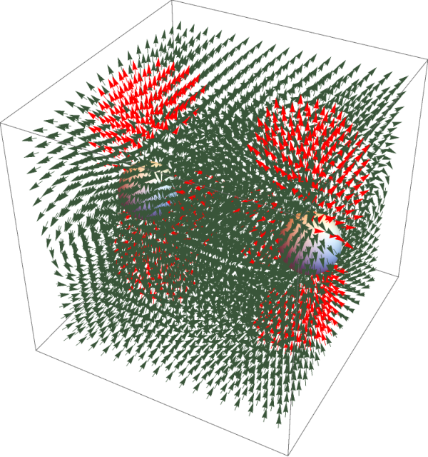
Let us assume that the stars are located at coordinate and are orbiting each other in the plane (so the orbital spin is along z-axis). (We neglect the sizes of the stars - the corresponding electromagnetic effects that take into account the size of the neutron stars were considered in §III). Below we will mostly plot 2D images in the plane (defined by the spin axis and the line connecting the stars, in the plane of the stars) and the plane (orthogonal to the line connecting the stars, passing through the center of mass). Results for the parallel case i are plotted in Fig. 4.
In the case of orbiting neutron stars with magnetic moments aligned with the orbital spin, there is some time dependence in the structure of the magnetosphere, but our prescription for estimating the preferred direction of the emission (see below) consistently predict emission along the spin axis, and hence no time variation. Nearly constant weak high energy or radio emission will be hard to detect observationally.
IV.4 Case ii: one magnetic moment parallel to the orbital spin and another in the plane of the orbit
For this configuration the magnetic and electric fields are plotted in Fig. 5.
IV.5 Case ii: time dependence
In contrast to the cases-i, the cases-ii are highly time dependent, as the system will evolve from ii-a, to ii-b, to “minus” ii-a, “minus” ii-b (by “minus” we mean the relative orientation of the magnetic moment with respect to the line of sight). Thus, if the spins of the neutron stars are misaligned with the orbital spin, the structure if the magnetosphere will change quasi-periodically on the orbital time scale. This may result in periodically changing emission.
At the present state, we cannot predict radio emission properties given the macroscopic electromagnetic structure of the magnetosphere. Hence, we must resolve to probable emission indicators to predict the light curves. Let us choose the value of the parallel electric field as a proxy for the directional properties of radio emission. For any configuration we know , Eq (22) and Fig. 6. Let us assume that emission is produced along the magnetic field line at the point of maximal within the magnetosphere. As a function of the polar angle and the azimuthal angle the resulting emission will have a complicated patter, Fig 7.


In both plots in Fig. 7 several curves arise because the code is looking for a global maximum but occasionally gets “trapped” in the local ones. This also indicates that emission may/could change sporadically, appearing at different field lines.
Finally, we note that in the 2M-DNS configuration (it may become zero at some discreet number of point).
IV.6 2M-DNS - reconnection flares at corotation
If the stars are rotating, there is another possibility for the production of radiation due to linking of the two magnetospheres at the time when the orbital period matches the pulsar’s rotational period - at corotation. [Magnetospheric interaction in close RS CVn binaries, e.g. 35, happens in this regime of near-corotation, whereby two stars can establish magnetic connections.]
Equating neutron star spin (1) with the orbital frequency at time before the merger
| (27) |
the corotating occurs at time
| (28) |
At the time the stars are separated by
| (29) |
If two stars are in approximate corotation, there is time for magnetospheric field lines to reconnect, creating a link between the two stars. We stress that the stars become magnetically connected not due to the diffusive processes in the crust, but due to reconnection in the common magnetosphere, see Fig. 8.
After two stars established magnetic connection, the common field lines will be stretched due to (small) mismatch in the corotation condition. This mechanism puts some of the energy of the orbital motion in the magnetic field. After a critical value of magnetic bending, instabilities will disrupt the magnetic bridge between. In the process part of the magnetic energy of the flux tube will be dissipated.
The total magnetic energy of a flux tube connecting two stars can be estimated as
| (30) |
This is a fairly small amount of energy, unlikely to be detectable (unless a large fraction is put into radio).
IV.7 A step towards a plasma model of interacting magnetospheres
The above considerations were based on the vacuum assumption. Appearance of parallel electric fields, as well as regions with , will lead to pair production. As a result the global plasma dynamics will be (could be) described by a plasma (MHD or relativistic force-free) approximation. As a step towards plasma models let us estimate typical current densities and the corresponding charge density.
Two lines of reasoning give the bracketing estimates of the plasma density in the 2M-DNS model. First, the typical current and charge density in the magnetosphere can be estimated as
| (31) |
which has a clear relation to the Goldreich-Julian density. Density , Eq. (31), is the charge density we expect in the magnetospheres of interacting neutron stars.
Second, in the time-dependent configuration 2M-DNS, equating typical to the electric current (in proper units), we find
| (32) |
where , , is the average magnetic field in the immediate surrounding of the neutron stars, and we used (recall that is the (semi)-separation between the stars). Thus, time-dependence induces a weaker requirement on the charge density, similar to the pulsar magnetosphere case.
By the nature of our vacuum approximation, the expected plasma current is fairly distributed. After the plasma is produces, narrow current sheets may/will be formed, leading to intermittent, and possibly explosive relativistic reconnection [22, 20, 21], particle acceleration, and production of the non-thermal radiation. Thus, we expect that magnetospheric interaction produces flares.
IV.8 The last few minutes: possible compactness shroud
As the neutron stars spiral in, the potential and the total luminosity increase. As some point before the merger the compactness parameter,
| (33) |
becomes larger than unity. This occurs at
| (34) |
Qualitatively, when the compactness parameter becomes larger than unity a large fraction of energy is converted into pairs that form an optically dense plasma that in turn may shroud the central neutron stars [25].
If the shrouding indeed occurs, this will be a bad news for a possibility to observe the precursors, since (i) the luminosity of the expected GRB-like outflow from the shroud will be small - of the total luminosity (23), which is already small, most energy will be spent on flow acceleration and not on the production of emission [10, recall the low efficiency problem of early theories of GRB outflows]; (ii) the shroud will redistribute possibly directed emission from gaps/reconnection cites into isotropic fireball, preventing orbital modulation; (iii) shrouding is likely to pollute the gaps and prevent generation of coherent radio emission.
It is far from clear that shrouding would indeed occur since the estimate (33): (i) is based on the total Poynting luminosity, the real electromagnetic luminosity will be smaller, resulting in smaller ; assumes that most of the luminosity initially comes out in pair-producing photons with energy MeV; assumes that radiation processes are isotropic - anisotropic particle acceleration in the gaps/current sheets will produce anisotropic photon distribution which will reduce pair production efficiency.
V Discussion
In this paper we argue that an effective “friction” of the of magnetospheres due to the orbital motion can revive pair production and lead to generation of electromagnetic emission. We demonstrate that the interaction of the magnetic fields of the merging neutron stars can create vacuum gaps, somewhat akin to the outer gaps in pulsar magnetospheres [5, 32], and reconnection sheets. The total available potentials in merging neutron stars (Eqns. (7)-(23)) are larger that what is need to produce pairs (sufficiently close to the merger), these parallel electric fields, and regions with , will result in pair production, that will screen them, and reduce the problem to the plasma case of . In the process, this will (may) create particle distributions that are unstable to the generation of radio waves.
The problem of pulsar radio emission - generation of radio waves by a relativistic unipolar inductor - is notoriously complicated. It is a general agreement that parallel electric fields are needed. Particles will be accelerated in the gaps, and under certain conditions can generate a dense secondary pair plasma. Plasma instabilities [23, 19, 24, e.g.] then may lead to the generation of coherent radio emission.
The active stage of the DNS merger, when LIGO gets an appreciable signal, lasts for seconds [1]; hence there may be enough time for radio observations, e.g. with LOFAR. LOFAR can see the whole sky at a given time, especially with its low frequency antennas (LBAs, 10-90MHz); the high frequency antennas (HBAs, 110-240MHz) can see the 20 degree-wide field. The data rate is huge, so that phase correlations are mostly done in real time; there is a possibility to have data stored using the Transient Buffer Boards, to be linked to transients’ notifications. The low frequency radio waves can also be delayed by tens of seconds due to plasma dispersion effects, possibly giving extra time for responses to the notification of a transient.
Acknowledgments
This work had been supported NSF grant AST-1306672, DoE grant DE-SC0016369 and NASA grant 80NSSC17K0757.
ML would like to thank Dimitrios Giannios, Jason Hessels, Stephen Reynolds and Joeri van Leeuven for discussions, and organizers and participants of the Plasma Physics of Neutron Star Mergers workshop.
References
- [1] Abbott, B. P., Abbott, R., Abbott, T. D., Acernese, F., Ackley, K., Adams, C., Adams, T., Addesso, P., Adhikari, R. X., Adya, V. B., & et al. 2017, Physical Review Letters, 119, 161101
- [2] Baiotti, L., & Rezzolla, L. 2017, Reports on Progress in Physics, 80, 096901
- [3] Bildsten, L., & Cutler, C. 1992, ApJ, 400, 175
- [4] Blandford, R. D. 2002, in Lighthouses of the Universe: The Most Luminous Celestial Objects and Their Use for Cosmology, ed. M. Gilfanov, R. Sunyeav, & E. Churazov, 381
- [5] Cheng, K. S., Ho, C., & Ruderman, M. 1986, ApJ, 300, 500
- [6] de Jager, O. C., Harding, A. K., Michelson, P. F., Nel, H. I., Nolan, P. L., Sreekumar, P., & Thompson, D. J. 1996, ApJ, 457, 253
- [7] Fawley, W. M., Arons, J., & Scharlemann, E. T. 1977, ApJ, 217, 227
- [8] Gehrels, N. et al. . 2004, ApJ, 611, 1005
- [9] Goldreich, P., & Julian, W. H. 1969, ApJ, 157, 869
- [10] Goodman, J. 1986, ApJ, 308, L47
- [11] Hansen, B. M. S., & Lyutikov, M. 2001, MNRAS, 322, 695
- [12] Hibschman, J. A., & Arons, J. 2001, ApJ, 560, 871
- [13] Lai, D. 2012, ApJ, 757, L3
- [14] Levinson, A., Melrose, D., Judge, A., & Luo, Q. 2005, ApJ, 631, 456
- [15] Lyutikov, M. 2006, New Journal of Physics, 8, 119
- [16] —. 2011a, Phys. Rev. D, 83, 124035
- [17] —. 2011b, Phys. Rev. D, 83, 064001
- [18] Lyutikov, M., Komissarov, S., & Sironi, L. 2018, Journal of Plasma Physics, 84, 635840201
- [19] Lyutikov, M., Machabeli, G., & Blandford, R. 1999, ApJ, 512, 804
- [20] Lyutikov, M., Sironi, L., Komissarov, S. S., & Porth, O. 2017a, Journal of Plasma Physics, 83, 635830601
- [21] —. 2017b, Journal of Plasma Physics, 83, 635830602
- [22] Lyutikov, M., & Uzdensky, D. 2003, ApJ, 589, 893
- [23] Melrose, D. B. 1989, Instabilities in Space and Laboratory Plasmas, ed. D. B. Melrose
- [24] Melrose, D. B. 2000, in Astronomical Society of the Pacific Conference Series, Vol. 202, IAU Colloq. 177: Pulsar Astronomy - 2000 and Beyond, ed. M. Kramer, N. Wex, & R. Wielebinski, 721–+
- [25] Metzger, B. D., & Zivancev, C. 2016, MNRAS, 461, 4435
- [26] Misner, C. W., Thorne, K. S., & Wheeler, J. A. 1973, Gravitation (San Francisco: W.H. Freeman and Co., 1973)
- [27] Palenzuela, C., Lehner, L., & Liebling, S. L. 2010, Science, 329, 927
- [28] Palenzuela, C., Lehner, L., Liebling, S. L., Ponce, M., Anderson, M., Neilsen, D., & Motl, P. 2013a, Phys. Rev. D, 88, 043011
- [29] Palenzuela, C., Lehner, L., Ponce, M., Liebling, S. L., Anderson, M., Neilsen, D., & Motl, P. 2013b, Physical Review Letters, 111, 061105
- [30] Ponce, M., Palenzuela, C., Barausse, E., & Lehner, L. 2015, Phys. Rev. D, 91, 084038
- [31] Ponce, M., Palenzuela, C., Lehner, L., & Liebling, S. L. 2014, Phys. Rev. D, 90, 044007
- [32] Romani, R. W. 1996, ApJ, 470, 469
- [33] Tan, C. M., Bassa, C. G., Cooper, S., Dijkema, T. J., Esposito, P., Hessels, J. W. T., Kondratiev, V. I., Kramer, M., Michilli, D., Sanidas, S., Shimwell, T. W., Stappers, B. W., van Leeuwen, J., Cognard, I., Grießmeier, J.-M., Karastergiou, A., Keane, E. F., Sobey, C., & Weltevrede, P. 2018, ArXiv e-prints
- [34] Timokhin, A. N. 2010, MNRAS, 408, 2092
- [35] Uchida, Y., & Sakurai, T. 1983, in Astrophysics and Space Science Library, Vol. 102, IAU Colloq. 71: Activity in Red-Dwarf Stars, ed. P. B. Byrne & M. Rodono, 629–632