跳到论文正文
W Papers独立论文阅读器 arXiv:1809.10451 论文正文 计算阅读时间 · 0%
引用这篇论文根据当前论文元数据生成,正式投稿前建议核对。


License: arXiv.org perpetual non-exclusive license
arXiv:1809.10451v1 [math-ph] 27 Sep 2018

Central limit theorems for open quantum random walks on the crystal lattices

Chul Ki Ko Note: University College, Yonsei University, 85 Songdogwahak-ro, Yeonsu-gu, Incheon 21983, Korea. E-mail: kochulki@yonsei.ac.kr    Norio Konno Note: Department of Applied Mathematics, Faculty of Engineering, Yokohama National University, Hodogaya, Yokohama 240-8501, Japan. E-mail: konno@ynu.ac.jp    Etsuo Segawa Note: Graduate School of Information Sciences, Tohoku University, 6-3-09 Aramaki Aza, Aoba, Sendai, Miyagi, 980-8579, Japan. E-mail: e-segawa@m.tohoku.ac.jp    Hyun Jae Yoo Note: Department of Applied Mathematics, Hankyong National University, 327 Jungang-ro, Anseong-si, Gyeonggi-do 17579, Korea. E-mail: yoohj@hknu.ac.kr Note: Corresponding author
Abstract

We consider the open quantum random walks on the crystal lattices and investigate the central limit theorems for the walks. On the integer lattices the open quantum random walks satisfy the central limit theorems as was shown by Attal, et al. In this paper we prove the central limit theorems for the open quantum random walks on the crystal lattices. We then provide with some examples for the Hexagonal lattices. We also develop the Fourier analysis on the crystal lattices. This leads to construct the so called dual processes for the open quantum random walks. It amounts to get Fourier transform of the probability densities, and it is very useful when we compute the characteristic functions of the walks. In this paper we construct the dual processes for the open quantum random walks on the crystal lattices providing with some examples.

Keywords. Open quantum random walks, crystal lattices, central limit theorem, dual processes.
2010 Mathematics Subject Classification: 82B41, 82C41, 82S22.

1 Introduction

The purpose of this paper is to construct the open quantum random walks on the crystal lattices and investigate the asymptotic behavior, namely central limit theorems.

The unitary quantum walks have been developed and applied as a tool for quantum algorithms, and it succeeded by its power of speeding up in certain search algorithms [1, 7, 8, 18]. Since it was mathematically formulated many properties of quantum walks have been known, especially the asymptotic behavior of the quantum walks was shown [2, 9, 10, 12, 13]. More precisely, it was proved that the quantum walks, when they are scaled by 1/n1/n, have limit distributions with certain densities, which are drastically different from Gaussian, the limit distributions of the classical randoms walks resulting from the central limit theorem [9, 12, 13].

Recently, a new type of quantum walks, so called open quantum random walks (OQRWs hereafter) was introduced [3, 4, 5]. The OQRWs were developed to formulate the dissipative quantum computing algorithms and dissipative quantum state preparation [5]. The decoherence and dissipation occur by the interaction of a system with environment and one needs to develop a proper quantum walk so that the dissipativity can be implemented. The works of [3, 4, 5] aim to fulfill this requirement. The OQRWs are not unitary evolutions of states, contrary to the early developed unitary quantum walks (it was thus named). By the procedure of quantum trajectories, which amounts to a repeated measurement of the particle at each step and an application of a completely positive map, the OQRWs are simulated by Markov chains on the product of position and state spaces [3, 4, 5] (see section 2 for the details).

In the paper [3], Attal et al. proved the central limit theorems for OQRWs on the integer lattice ℤd\mathbb{Z}^{d}. This result typically shows that the behavior of OQRWs and unitary quantum walks are much different. On the other hand, when we consider the dynamics on the integer lattices, we can develop Fourier transforms. In [14], Konno and Yoo developed the Fourier transform theory for the OQRWs on the integer lattices, and by it the so called dual process was constructed. It is in a sense the process of Fourier transforms of probability distributions. Some related works on the central limit theorems for OQRWs, one can find in the references [6, 16].

In this paper we construct OQRWs on the crystal lattices. The crystal lattices are the structures which have regularity globally, like integer lattices, but may have further structure locally (see subsection 2.1 for the definition). Therefore, not only the integer lattices belong to this class but more fruitful structures can be considered. The goal of the paper is two-fold: one is to show the central limit theorems for the OQRWs on the crystal lattices and the other is to construct the dual processes by using a Fourier transform theory on the crystal lattices. Following the superb method developed in [3] we could show the central limit theorems. We will provide with some examples for the Hexagonal lattices. We then develop a Fourier transform theory and construct the dual processes as was done in [14]. By revisiting the examples we will see that the central limit theorems can be also obtained by the dual processes. In some examples it even provides a better understanding of the dynamics. We remark that recently the present authors considered the orbits, or the support of the scaled unitary quantum walks on the crystal lattices [11].

This paper is organized as follows. In section 2 we introduce the crystal lattices and construct OQRWs on them. In section 3, we show the central limit theorems (Theorem 3.5). Section 4 is devoted to the examples. Typically we will consider Hexagonal lattices. We give two examples which have nonzero- and zero-covariances, respectively, in the limit. In section 5, we construct dual processes after a short introduction of Fourier analysis on the crystal lattices. The examples mentioned above are revisited for comparison. Appendix A gives a proof for the central limit theorem. We follow the methods in [3] with a suitable modification. In the Appendix B and C, we provide with analytic proofs for some technical results that are used in the examples.

2 OQRWs on the crystal lattices

2.1 Crystal lattices

In this subsection we introduce the crystal lattices as was done in [11]. Let G0=(V0,E0)G_{0}=(V_{0},E_{0}) be a finite graph which may have multi edges and self loops. We use the notation A⁡(G0)A(G_{0}) for the set of symmetric arcs induced by E0E_{0}. The homology group of G0G_{0} with integer coefficients is denoted by H1​(G0,ℤ)H_{1}(G_{0},\mathbb{Z}). The abstract periodic lattice 𝕃\mathbb{L} induced by a subgroup H⊂H1​(G0,ℤ)H\subset H_{1}(G_{0},\mathbb{Z}) is denoted by H1​(G0,ℤ)/HH_{1}(G_{0},\mathbb{Z})/H [17].

Let the set of basis of H1​(G0,ℤ)H_{1}(G_{0},\mathbb{Z}) be {C1,C2,…,Cb1}\{C_{1},C_{2},\dots,C_{b_{1}}\} corresponding to fundamental cycles of G0G_{0}, where b1b_{1} is the first Betti number of G0G_{0}. The spanning tree induced by {C1,C2,…,Cb1}\{C_{1},C_{2},\dots,C_{b_{1}}\} is denoted by 𝕋0\mathbb{T}_{0}. We can take a one-to-one correspondence between {C1,C2,…,Cb1}\{C_{1},C_{2},\dots,C_{b_{1}}\} and A​(𝕋0)cA(\mathbb{T}_{0})^{c}; we describe C⁡(e)∈{C1,C2,…,Cb1}C(e)\in\{C_{1},C_{2},\dots,C_{b_{1}}\} as the fundamental cycle corresponding to e∈A​(𝕋0)ce\in A(\mathbb{T}_{0})^{c} so that C⁡(e)C(e) is the cycle generated by adding ee to 𝕋0\mathbb{T}_{0}. Let dd be the number of generators of the quotient group H1​(G0,ℤ)/HH_{1}(G_{0},\mathbb{Z})/H. By taking a set of generating vectors {θ^​(e):e∈A​(𝕋0)c}\{\widehat{\theta}(e):e\in A(\mathbb{T}_{0})^{c}\} (we suppose θ^​(e¯)=−θ^​(e)\widehat{\theta}(\bar{e})=-\widehat{\theta}(e), where e¯\bar{e} means the reversed arc of ee), we may consider 𝕃\mathbb{L} as a subset of ℝd\mathbb{R}^{d} isomorphic to ℤd\mathbb{Z}^{d} . In other words, we may think

𝕃={∑neθ^(e):e∈A(𝕋0)c,ne∈ℤ}.\mathbb{L}=\left\{\sum n_{e}\widehat{\theta}(e):e\in A(\mathbb{T}_{0})^{c},\,\,n_{e}\in\mathbb{Z}\right\}.

Let us define a covering graph G=(V,A)G=(V,A) of G0G_{0} by the lattice 𝕃\mathbb{L}. For it, define ϕ:A⁡(𝕋0)→ℝd\phi:A(\mathbb{T}_{0})\to\mathbb{R}^{d} so that ϕ⁡(e¯)=−ϕ⁡(e)\phi(\bar{e})=-\phi(e) for every e∈A0e\in A_{0}. We also define ϕ0:V0→ℝd\phi_{0}:V_{0}\to\mathbb{R}^{d} so that ϕ⁡(e)=ϕ0​(t⁡(e))−ϕ0​(o⁡(e))\phi(e)=\phi_{0}(\mathrm{t}(e))-\phi_{0}(\mathrm{o}(e)) for every e∈A⁡(𝕋0)e\in A(\mathbb{T}_{0}) by fixing a point ϕ0​(v0)\phi_{0}(v_{0}) at some vertex v0∈V0v_{0}\in V_{0}. Here t⁡(e)\mathrm{t}(e) and o⁡(e)\mathrm{o}(e) denote the terminal and origin of the arc ee, respectively. Now the covering graph G=(V,A)G=(V,A) is defined as follows.

V\displaystyle V =\displaystyle= 𝕃+ϕ0​(V0)≅𝕃×ϕ0​(V0);\displaystyle\mathbb{L}+\phi_{0}(V_{0})\cong\mathbb{L}\times\phi_{0}(V_{0});
A\displaystyle A =\displaystyle= ∪x∈𝕃{((x,o(e)),(x,t(e)))|e∈A(𝕋0)}\displaystyle\cup_{x\in\mathbb{L}}\left\{\left((x,\mathrm{o}(e)),(x,\mathrm{t}(e))\right)\;|\;e\in A(\mathbb{T}_{0})\right\}
∪(∪x∈𝕃{((x,o(e)),(x+θ^(e),t(e)))|e∈Ac(𝕋0)}).\displaystyle\quad\cup\left(\cup_{x\in\mathbb{L}}\left\{\left((x,\mathrm{o}(e)),(x+\widehat{\theta}(e),\mathrm{t}(e))\right)\;|\;e\in A^{c}(\mathbb{T}_{0})\right\}\right).

The covering graph G=(V,A)G=(V,A) is called a crystal lattice.

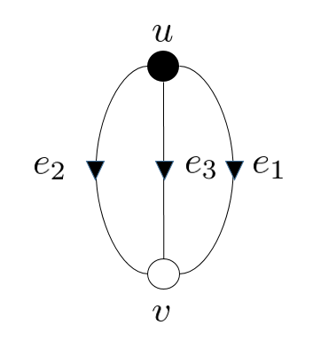
Refer to caption
Refer to caption
Figure 1: Hexagonal lattice: underlying graph G0G_{0} for Hexagonal lattice (left), Hexagonal lattice (right)

We take θ^​(e)≡0\widehat{\theta}(e)\equiv 0 for e∈A⁡(𝕋0)e\in A(\mathbb{T}_{0}) and choose ei1,…,eide_{i_{1}},\dots,e_{i_{d}} from A​(𝕋0)cA(\mathbb{T}_{0})^{c} so that θ^1:=θ^​(ei1),…,θ^d:=θ^​(eid)\widehat{\theta}_{1}:=\widehat{\theta}(e_{i_{1}}),\dots,\widehat{\theta}_{d}:=\widehat{\theta}(e_{i_{d}}) span ℝd\mathbb{R}^{d}. We further suppose that for all e∈A⁡(G0)e\in A(G_{0}), θ^(e)∈{∑i=1dniθ^i:ni∈ℤ,i=1,⋯,d}\widehat{\theta}(e)\in\{\sum_{i=1}^{d}n_{i}\widehat{\theta}_{i}:n_{i}\in\mathbb{Z},\,i=1,\cdots,d\}, and for any two arcs eie_{i} and eje_{j} in A​(𝕋0)cA(\mathbb{T}_{0})^{c}, θ^​(ei)\widehat{\theta}(e_{i}) and θ^​(ej)\widehat{\theta}(e_{j}) are linearly independent unless ej=e¯ie_{j}=\overline{e}_{i}. We define a d×dd\times d matrix by

Θ:=([θ^1,…,θ^d]−1)T.\Theta:=([\widehat{\theta}_{1},\dots,\widehat{\theta}_{d}]^{-1})^{T}. (2.1)

Notice that if {𝐞i:i=1,⋯,d}\{{\bf e}_{i}:i=1,\cdots,d\} is the canonical basis for ℝd\mathbb{R}^{d}, then we have

𝐞i=∑j=1dΘi​j​θ^j.{\bf e}_{i}=\sum_{j=1}^{d}\Theta_{ij}\widehat{\theta}_{j}. (2.2)

The matrix Θ\Theta will take a crucial role when we consider Fourier transforms.

2.2 OQRWs on the crystal lattices

We let 𝒦:=l2​(𝕃)\mathcal{K}:=l^{2}(\mathbb{L}) and by {|x⟩:x∈𝕃}\{|x\rangle:x\in\mathbb{L}\} we denote the canonical orthonormal basis of 𝒦\mathcal{K}. Let ℋ\mathcal{H} be a finite dimensional Hilbert space and for each u∈V0u\in V_{0}, let ℋu\mathcal{H}_{u} be a copy of ℋ\mathcal{H}. Define

𝔥:=⊕u∈V0ℋu.\mathfrak{h}:=\oplus_{u\in V_{0}}\mathcal{H}_{u}.

𝔥\mathfrak{h} represents an intrinsic structure at each site of 𝕃\mathbb{L}. The Hilbert space 𝔥⊗𝒦\mathfrak{h}\otimes\mathcal{K} is the base Hilbert space on which our OQRWs are working. For each e∈A⁡(G0)e\in A(G_{0}), e=(u,v)e=(u,v), we let B⁡(e)B(e) be a bounded linear operator from ℋu\mathcal{H}_{u} to ℋv\mathcal{H}_{v} satisfying

∑e∈A⁡(G0);o⁡(e)=uB∗​(e)​B​(e)=Iℋufor all ​u∈V0.\sum_{\begin{subarray}{c}e\in A(G_{0});\\ \mathrm{o}(e)=u\end{subarray}}B^{*}(e)B(e)=I_{\mathcal{H}_{u}}\quad\text{for all }u\in V_{0}. (2.3)

Whenever there is no danger of confusion we also understand ℋu\mathcal{H}_{u} as a subspace of 𝔥\mathfrak{h}. With this convention, B⁡(e)B(e) (using the same symbol by abuse of notations) is a bounded linear operator on 𝔥\mathfrak{h} and satisfies

∑e∈A⁡(G0)B∗​(e)​B​(e)=∑u∈V0∑e∈A⁡(G0);o⁡(e)=uB∗​(e)​B​(e)=∑u∈V0Iℋu=I𝔥.\sum_{e\in A(G_{0})}B^{*}(e)B(e)=\sum_{u\in V_{0}}\sum_{\begin{subarray}{c}e\in A(G_{0});\\ \mathrm{o}(e)=u\end{subarray}}B^{*}(e)B(e)=\sum_{u\in V_{0}}I_{\mathcal{H}_{u}}=I_{\mathfrak{h}}. (2.4)

The operators {B⁡(e):e∈A⁡(G0)}\{B(e):e\in A(G_{0})\} will constitute the Kraus representation of our OQRWs on the crystal lattices. For that we define for each x∈𝕃x\in\mathbb{L} and e∈A⁡(G0)e\in A(G_{0}), a bounded linear operator LxeL_{x}^{e} on 𝔥⊗𝒦\mathfrak{h}\otimes\mathcal{K} by

Lxe:=B⁡(e)⊗|x+θ^​(e)⟩​⟨x|.L_{x}^{e}:=B(e)\otimes|x+\widehat{\theta}(e)\rangle\langle x|. (2.5)

We can check the following property.

Lemma 2.1
∑x∈𝕃∑e∈A⁡(G0)(Lxe)∗​Lxe=I𝔥⊗𝒦.\sum_{x\in\mathbb{L}}\sum_{e\in A(G_{0})}\left(L_{x}^{e}\right)^{*}L_{x}^{e}=I_{\mathfrak{h}\otimes\mathcal{K}}. (2.6)

Proof. By (2.4),

∑x∈𝕃∑e∈A⁡(G0)(Lxe)∗​Lxe\displaystyle\sum_{x\in\mathbb{L}}\sum_{e\in A(G_{0})}\left(L_{x}^{e}\right)^{*}L_{x}^{e} =\displaystyle= ∑x∈𝕃∑e∈A⁡(G0)B​(e)∗​B​(e)⊗|x⟩​⟨x|\displaystyle\sum_{x\in\mathbb{L}}\sum_{e\in A(G_{0})}B(e)^{*}B(e)\otimes|x\rangle\langle x|
=\displaystyle= ∑x∈𝕃I𝔥⊗|x⟩​⟨x|\displaystyle\sum_{x\in\mathbb{L}}I_{\mathfrak{h}}\otimes|x\rangle\langle x|
=\displaystyle= I𝔥⊗𝒦.\displaystyle I_{\mathfrak{h}\otimes\mathcal{K}}.

□\Box

The OQRW is a completely positive linear operator on the ideal ℐ1\mathcal{I}_{1} of trace class operators on 𝔥⊗𝒦{\mathfrak{h}\otimes\mathcal{K}} defined by

ℳ⁡(ρ):=∑x∈𝕃∑e∈A⁡(G0)Lxe​ρ​(Lxe)∗.\mathcal{M}(\rho):=\sum_{x\in\mathbb{L}}\sum_{e\in A(G_{0})}L_{x}^{e}\rho(L_{x}^{e})^{*}. (2.7)

Let us consider a special class of states (density operators) on 𝔥⊗𝒦\mathfrak{h}\otimes\mathcal{K} of the form

ρ=∑x∈𝕃(⊕u∈V0ρ(x,u))⊗|x⟩⟨x|.\rho=\sum_{x\in\mathbb{L}}\left(\oplus_{u\in V_{0}}\rho_{(x,u)}\right)\otimes|x\rangle\langle x|. (2.8)

Here, for each pair (x,u)∈𝕃×V0(x,u)\in\mathbb{L}\times V_{0}, ρ(x,u)\rho_{(x,u)} is a positive definite operator on ℋu\mathcal{H}_{u} and satisfies

∑x∈𝕃∑u∈V0Tr​(ρ(x,u))=1.\sum_{x\in\mathbb{L}}\sum_{u\in V_{0}}\text{Tr}(\rho_{(x,u)})=1.

The value ∑u∈V0Tr​(ρ(x,u))\sum_{u\in V_{0}}\text{Tr}(\rho_{(x,u)}) is understood as a probability of finding the particle at site x∈𝕃x\in\mathbb{L} when the state is ρ\rho. We check that if the state has the form in (2.8), ρ=∑x∈𝕃(⊕u∈V0ρ(x,u))⊗|x⟩⟨x|\rho=\sum_{x\in\mathbb{L}}\left(\oplus_{u\in V_{0}}\rho_{(x,u)}\right)\otimes|x\rangle\langle x|, ℳ⁡(ρ)\mathcal{M}(\rho) has the form

ℳ(ρ)=∑x∈𝕃(⊕u∈V0ρ(x,u)′)⊗|x⟩⟨x|,\mathcal{M}(\rho)=\sum_{x\in\mathbb{L}}\left(\oplus_{u\in V_{0}}\rho^{\prime}_{(x,u)}\right)\otimes|x\rangle\langle x|, (2.9)

where

ρ(x,u)′=∑e∈A⁡(G0);t⁡(e)=uB⁡(e)​ρ(x−θ^​(e),o​(e))​B​(e)∗.\rho^{\prime}_{(x,u)}=\sum_{\begin{subarray}{c}e\in A(G_{0});\\ \mathrm{t}(e)=u\end{subarray}}B(e)\rho_{(x-\widehat{\theta}(e),\mathrm{o}(e))}B(e)^{*}.

From now on we assume that ℳ\mathcal{M} is defined on the set of states of the form in (2.8).

Let XX denote the random variable representing the position of the particle, or the walker. Starting from the initial state ρ\rho in (2.8), the probability of finding the particle at site x∈𝕃x\in\mathbb{L} after a one-step evolution is given by

ℙ⁡(X=x)=∑u∈V0Tr​(ρ(x,u)′).\mathbb{P}(X=x)=\sum_{u\in V_{0}}\text{Tr}(\rho^{\prime}_{(x,u)}).

As was introduced in [3, 4], let (ρn,Xn)n≥0(\rho_{n},X_{n})_{n\geq 0} denote the Markov chain of quantum trajectory procedure. This is obtained by repeatedly applying the completely positive map ℳ\mathcal{M} and a measurement of the position on 𝒦\mathcal{K}. More precisely, denoting ℰ⁡(𝔥)\mathcal{E}(\mathfrak{h}) the space of states on 𝔥\mathfrak{h}, (ρn,Xn)n≥0(\rho_{n},X_{n})_{n\geq 0} is a Markov chain on the state space ℰ⁡(𝔥)×𝕃\mathcal{E}(\mathfrak{h})\times\mathbb{L} for which the transition rule is defined as follows: from a point (ρ,x)∈ℰ⁡(𝔥)×𝕃(\rho,x)\in\mathcal{E}(\mathfrak{h})\times\mathbb{L} it jumps to the point

(1p⁡(e)​B​(e)​ρ​B​(e)∗,x+θ^​(e))∈ℰ⁡(𝔥)×𝕃,\left(\frac{1}{p(e)}B(e)\rho B(e)^{*},x+\widehat{\theta}(e)\right)\in\mathcal{E}(\mathfrak{h})\times\mathbb{L},

with probability

p⁡(e)=Tr​(B⁡(e)​ρ​B​(e)∗).p(e)=\text{Tr}(B(e)\rho B(e)^{*}).

3 Central limit theorem

In this section we discuss the central limit theorem for the OQRWs on the crystal lattices. The same study for the OQRWs on the integer lattices ℤd\mathbb{Z}^{d} was done in [3]. Here we follow the same stream lines of [3] with slight modifications.

3.1 Preparation

We let

ℒ⁡(ρ):=∑e∈A⁡(G0)B⁡(e)​ρ​B​(e)∗,ρ∈ℰ⁡(𝔥).\mathcal{L}(\rho):=\sum_{e\in A(G_{0})}B(e)\rho B(e)^{*},\quad\rho\in\mathcal{E}(\mathfrak{h}). (3.1)

We assume the following hypothesis.

  1. (H)

    ℒ\mathcal{L} admits a unique invariant state ρ∞\rho_{\infty}.

Remark 3.1

The existence of an invariant state to the equation (3.1) follows from an ergodic theorem [15]. In fact, for any initial state ρ0\rho_{0}, the time average

1n​∑k=0n−1ℒk​(ρ0)\frac{1}{n}\sum_{k=0}^{n-1}\mathcal{L}^{k}(\rho_{0})

converges almost surely (in a suitable probability space) to an invariant state ρ∞∈ℰ⁡(𝔥)\rho_{\infty}\in\mathcal{E}(\mathfrak{h}) (see also [3]).

Let us define

m:=∑e∈A⁡(G0)Tr​(B⁡(e)​ρ∞​B​(e)∗)​θ^​(e).m:=\sum_{e\in A(G_{0})}\text{Tr}\left(B(e)\rho_{\infty}B(e)^{*}\right)\widehat{\theta}(e). (3.2)
Lemma 3.2

For any l∈ℝdl\in\mathbb{R}^{d}, the equation

L−ℒ∗​(L)=∑e∈A⁡(G0)B​(e)∗​B​(e)​(θ^​(e)⋅l)−(m⋅l)​IL-{\mathcal{L}}^{*}(L)=\sum_{e\in A(G_{0})}B(e)^{*}B(e)\left(\widehat{\theta}(e)\cdot l\right)-(m\cdot l)I (3.3)

admits a solution. The difference between any two solutions of (3.3) is a multiple of the identity.

Proof. By (3.2) we have for any l∈ℝdl\in\mathbb{R}^{d},

∑e∈A⁡(G0)Tr​(B⁡(e)​ρ∞​B​(e)∗)​θ^​(e)⋅l=m⋅l.\sum_{e\in A(G_{0})}\text{Tr}\left(B(e)\rho_{\infty}B(e)^{*}\right)\widehat{\theta}(e)\cdot l=m\cdot l.

Hence

Tr​(ρ∞​(∑e∈A⁡(G0)B​(e)∗​B​(e)​θ^​(e)⋅l−(m⋅l)​I))=0.\text{Tr}\Big(\rho_{\infty}\Big(\sum_{e\in A(G_{0})}B(e)^{*}B(e)\widehat{\theta}(e)\cdot l-\big(m\cdot l\big)I\Big)\Big)=0.

Thus

∑e∈A⁡(G0)B​(e)∗​B​(e)​(θ^​(e)⋅l)−(m⋅l)​I∈{ρ∞}⟂=Ran⁡(I−ℒ∗).\sum_{e\in A(G_{0})}B(e)^{*}B(e)\left(\widehat{\theta}(e)\cdot l\right)-\big(m\cdot l\big)I\in\{\rho_{\infty}\}^{\perp}=\mathrm{Ran}(I-{\mathcal{L}}^{*}).

The last equality follows from the fact that

{ρ∞}⟂=Ker​(I−ℒ)⟂=Ran⁡(I−ℒ∗)¯=Ran⁡(I−ℒ∗),\{\rho_{\infty}\}^{\perp}=\mathrm{Ker}(I-\mathcal{L})^{\perp}=\overline{\mathrm{Ran}(I-{\mathcal{L}^{*}})}=\mathrm{Ran}(I-{\mathcal{L}}^{*}),

since 𝔥\mathfrak{h} is of finite dimensional. This proves the first part. The second part can be proven by the same argument that was used in [3, Lemma 5.1]. □\Box

Let us denote the solution of (3.3) corresponding to ll by LlL_{l}. In particular, for the basis vectors {θ^1,⋯,θ^d}\{\widehat{\theta}_{1},\cdots,\widehat{\theta}_{d}\} of the lattice 𝕃\mathbb{L}, we denote LiL_{i} for Lθ^iL_{\widehat{\theta}_{i}}, i=1,⋯,di=1,\cdots,d. Note that

Ll=∑i=1dli​Li,L_{l}=\sum_{i=1}^{d}l_{i}L_{i}, (3.4)

where {li}\{l_{i}\} are the coordinates of ll w.r.t. {θ^i}\{\widehat{\theta}_{i}\}.

Recall the Markov chain (ρn,Xn)n≥0(\rho_{n},X_{n})_{n\geq 0} on the state space ℰ⁡(𝔥)×𝕃\mathcal{E}(\mathfrak{h})\times\mathbb{L}. We introduce a related Markov chain. The Markov chain (ρn,Yn)n≥0(\rho_{n},Y_{n})_{n\geq 0} is defined on the state space ℰ⁡(𝔥)×A⁡(G0)\mathcal{E}(\mathfrak{h})\times A(G_{0}). The transition probabilities are given as follows. From the state (ρ,e)(\rho,e), it jumps to (ρ′,e′)(\rho^{\prime},e^{\prime}) with probability Tr​(B⁡(e′)​ρ​B​(e′)∗)\text{Tr}(B(e^{\prime})\rho B(e^{\prime})^{*}), where ρ′=1Tr​(B⁡(e′)​ρ​B​(e′)∗)​(B⁡(e′)​ρ​B​(e′)∗)\rho^{\prime}=\frac{1}{\text{Tr}(B(e^{\prime})\rho B(e^{\prime})^{*})}(B(e^{\prime})\rho B(e^{\prime})^{*}). Notice that if we put Δ​Xn:=Xn−Xn−1∈{θ^​(e):e∈A⁡(G0)}\Delta X_{n}:=X_{n}-X_{n-1}\in\{\widehat{\theta}(e):\,e\in A(G_{0})\}, then (ρn,Δ​Xn)n≥0(\rho_{n},\Delta X_{n})_{n\geq 0} is a Markov chain that is equivalent with (ρn,θ^​(Yn))n≥0(\rho_{n},\widehat{\theta}(Y_{n}))_{n\geq 0}. The Markov operator (transition operator) for the Markov chain (ρn,Yn)n≥0(\rho_{n},Y_{n})_{n\geq 0} is denoted by PP.

Remark 3.3

We emphasize here that if (ρ,e)(\rho,e) is the present state for the Markov chain (Yn)(Y_{n}) and particularly if ρ\rho is supported on ℋu\mathcal{H}_{u} for some u∈V0u\in V_{0} (recall that 𝔥=⊕u∈V0ℋu\mathfrak{h}=\oplus_{u\in V_{0}}\mathcal{H}_{u}), then it jumps to some (ρ′,e′)(\rho^{\prime},e^{\prime}) where e′e^{\prime} must satisfy o⁡(e)=u\mathrm{o}(e)=u, since B⁡(e′)​ρ​B​(e′)∗=0B(e^{\prime})\rho B(e^{\prime})^{*}=0 if o⁡(e′)≠u\mathrm{o}(e^{\prime})\neq u.

Let us consider the Poisson equation [3]:

(I−P)​f​(ρ,e)=θ^​(e)⋅l−m⋅l.(I-P)f(\rho,e)=\widehat{\theta}(e)\cdot l-m\cdot l. (3.5)
Lemma 3.4

The equation (3.5) admits a solution which is

f⁡(ρ,e)=Tr⁡(ρ​Ll)+θ^​(e)⋅l.f(\rho,e)=\mathrm{Tr}(\rho L_{l})+\widehat{\theta}(e)\cdot l.

Proof. For the function f⁡(ρ,e)f(\rho,e) in the statement, we have

(I−P)​f​(ρ,e)\displaystyle(I-P)f(\rho,e) =\displaystyle= Tr⁡(ρ​Ll)+θ^​(e)⋅l\displaystyle\mathrm{Tr}(\rho L_{l})+\widehat{\theta}(e)\cdot l
−∑e′∈A⁡(G0)(Tr(B(e′)ρB(e′)∗Ll)+Tr(B(e′)ρB(e′)∗)θ^(e′)⋅l)\displaystyle-\sum_{e^{\prime}\in A(G_{0})}\Big(\text{Tr}\big(B(e^{\prime})\rho B(e^{\prime})^{*}L_{l}\big)+\text{Tr}\big(B(e^{\prime})\rho B(e^{\prime})^{*}\big)\widehat{\theta}(e^{\prime})\cdot l\Big)
=\displaystyle= Tr​(ρ⁡(Ll−ℒ∗​(Ll)−∑e′∈A⁡(G0)B​(e′)∗​B​(e′)​θ^​(e′)⋅l))+θ^​(e)⋅l\displaystyle\text{Tr}\Big(\rho\Big(L_{l}-{\mathcal{L}}^{*}(L_{l})-\sum_{e^{\prime}\in A(G_{0})}B(e^{\prime})^{*}B(e^{\prime})\widehat{\theta}(e^{\prime})\cdot l\Big)\Big)+\widehat{\theta}(e)\cdot l
=\displaystyle= θ^​(e)⋅l−m⋅l.\displaystyle\widehat{\theta}(e)\cdot l-m\cdot l.

The proof is completed. □\Box

3.2 Central limit theorem

In this subsection we present the central limit theorem for the OQRWs on the crystal lattices. All the ingredients needed to show the central limit theorem are prepared in the previous subsection. The main result of this paper is the following theorem.

Theorem 3.5

Consider the open quantum random walk on a crystal lattice (embedded in ℝd\mathbb{R}^{d}). Assume that the completely positive map

ℒ⁡(ρ)=∑e∈A⁡(G0)B⁡(e)​ρ​B​(e)∗\mathcal{L}(\rho)=\sum_{e\in A(G_{0})}B(e)\rho B(e)^{*}

admits a unique invariant state ρ∞\rho_{\infty} on 𝔥\mathfrak{h}. Let (ρn,Xn)n≥0(\rho_{n},X_{n})_{n\geq 0} be the quantum trajectory process associated to this OQRW. Then,

Xn−n​mn\frac{X_{n}-nm}{\sqrt{n}}

converges in law to the Gaussian distribution N⁡(0,Σ)N(0,\Sigma) in ℝd\mathbb{R}^{d}, with covariance matrix Σ=(Ci​j)i,j=1d\Sigma=(C_{ij})_{i,j=1}^{d} given by

Ci​j\displaystyle C_{ij} =\displaystyle= −mi​mj+∑e∈A⁡(G0)Tr​(B⁡(e)​ρ∞​B​(e)∗)​(θ^​(e))i​(θ^​(e))j\displaystyle-m_{i}m_{j}+\sum_{e\in A(G_{0})}\text{Tr}(B(e)\rho_{\infty}B(e)^{*})(\widehat{\theta}(e))_{i}(\widehat{\theta}(e))_{j} (3.6)
+2∑e∈A⁡(G0)Tr(B(e)ρ∞B(e)∗L𝐞i)(θ^(e))j−2miTr(ρ∞L𝐞j).\displaystyle+2\sum_{e\in A(G_{0})}\mathrm{Tr}(B(e)\rho_{\infty}B(e)^{*}L_{{\bf e}_{i}})(\widehat{\theta}(e))_{j}-2m_{i}\mathrm{Tr}(\rho_{\infty}L_{{\bf e}_{j}}).
Remark 3.6

Recall that {𝐞i}\{{\bf e}_{i}\} is the canonical basis of ℝd\mathbb{R}^{d} and Li=Lθ^iL_{i}=L_{\widehat{\theta}_{i}}. Since 𝐞i=∑j=1dΘi​j​θ^j{\bf e}_{i}=\sum_{j=1}^{d}\Theta_{ij}\widehat{\theta}_{j} (see (2.2)), we can compute L𝐞iL_{{\bf e}_{i}} by using LjL_{j}’s:

L𝐞i=∑j=1dΘi​j​Lj.L_{{\bf e}_{i}}=\sum_{j=1}^{d}{\Theta}_{ij}L_{j}.

In the real problems, it is generally easier to compute LiL_{i}’s than L𝐞iL_{{\bf e}_{i}}’s.

For the proof of the above theorem, it turns out that the methods are exactly the same as in [3]. We only have a different graph structure from integer lattices and need only to modify so that it is suitable for the new structure. For the readers’ convenience, however, we present the full proof in the Appendix A.

4 Examples: Hexagonal lattice

In this section we provide with some examples. We will consider the OQRWs on the hexagonal lattice. Look at the hexagonal lattice in Figure 1.

4.1 Preparation

We let V0={u,v}V_{0}=\{u,v\} and let {ei}i=1,2,3\{e_{i}\}_{i=1,2,3} be the three edges in G0G_{0} with o⁡(ei)=u\mathrm{o}(e_{i})=u and t⁡(ei)=v\mathrm{t}(e_{i})=v. (See Figure 1.) The reversed edges are e¯i\overline{e}_{i}, i=1,2,3i=1,2,3. We let

θ^​(e1)=12​(1,1),θ^​(e2)=12​(−1,1),θ^​(e3)=0,\widehat{\theta}(e_{1})=\frac{1}{\sqrt{2}}(1,1),\quad\widehat{\theta}(e_{2})=\frac{1}{\sqrt{2}}(-1,1),\quad\widehat{\theta}(e_{3})=0,

and θ^​(e¯i)=−θ^​(ei)\widehat{\theta}(\overline{e}_{i})=-\widehat{\theta}(e_{i}), i=1,2,3i=1,2,3. In order to define the operators B⁡(e)B(e), e∈A⁡(G0)e\in A(G_{0}), let ℋu=ℋv=ℂ3\mathcal{H}_{u}=\mathcal{H}_{v}=\mathbb{C}^{3}, and 𝔥=ℋu⊕ℋv≃ℂ6\mathfrak{h}=\mathcal{H}_{u}\oplus\mathcal{H}_{v}\simeq\mathbb{C}^{6}. Let U=[𝐮1𝐮2𝐮3]U=\left[\begin{matrix}{\bf u}_{1}&{\bf u}_{2}&{\bf u}_{3}\end{matrix}\right] and V=[𝐯1𝐯2𝐯3]V=\left[\begin{matrix}{\bf v}_{1}&{\bf v}_{2}&{\bf v}_{3}\end{matrix}\right] be 3×33\times 3 unitary matrices with column vectors 𝐮i=[u1​i,u2​i,u3​i]T{\bf u}_{i}=[u_{1i},u_{2i},u_{3i}]^{T} and 𝐯i=[v1​i,v2​i,v3​i]T{\bf v}_{i}=[v_{1i},v_{2i},v_{3i}]^{T}, i=1,2,3i=1,2,3. For i=1,2,3i=1,2,3, let UiU_{i} be a 3×33\times 3 matrix whose iith column is 𝐮i{\bf u}_{i} and remaining columns are zeros. Similarly, let ViV_{i} be the 3×33\times 3 matrix, whose iith column is the vector 𝐯i{\bf v}_{i} and other columns are zeros. For i=1,2,3i=1,2,3, let U~i\widetilde{U}_{i} and V~i\widetilde{V}_{i} be 6×66\times 6 matrices whose block matrices are given as follows:

U~i=[00Ui0],V~i=[0Vi00].\widetilde{U}_{i}=\left[\begin{matrix}0&0\\ U_{i}&0\end{matrix}\right],\quad\widetilde{V}_{i}=\left[\begin{matrix}0&V_{i}\\ 0&0\end{matrix}\right].

Now we define

B⁡(ei):=U~i,andB⁡(e¯i):=V~i,i=1,2,3.B(e_{i}):=\widetilde{U}_{i},\quad\text{and}\quad B(\overline{e}_{i}):=\widetilde{V}_{i},\quad i=1,2,3.

It is easy to check that a state ρ=ρu⊕ρv∈ℰ⁡(𝔥)\rho=\rho_{u}\oplus\rho_{v}\in\mathcal{E}(\mathfrak{h}) is an invariant state to the equation ℒ⁡(ρ)=ρ\mathcal{L}(\rho)=\rho, where ℒ⁡(ρ)\mathcal{L}(\rho) is defined in (3.1), if and only if it holds that

ρu=∑i=13Vi​ρv​Vi∗,\displaystyle\rho_{u}=\sum_{i=1}^{3}V_{i}\rho_{v}V_{i}^{*}, (4.1)
ρv=∑i=13Ui​ρu​Ui∗.\displaystyle\rho_{v}=\sum_{i=1}^{3}U_{i}\rho_{u}U_{i}^{*}. (4.2)

Consider the following (doubly) stochastic matrices.

Pu:=[|u11|2|u21|2|u31|2|u12|2|u22|2|u32|2|u13|2|u23|2|u33|2],Pv:=[|v11|2|v21|2|v31|2|v12|2|v22|2|v32|2|v13|2|v23|2|v33|2].P_{u}:=\left[\begin{matrix}|u_{11}|^{2}&|u_{21}|^{2}&|u_{31}|^{2}\\ |u_{12}|^{2}&|u_{22}|^{2}&|u_{32}|^{2}\\ |u_{13}|^{2}&|u_{23}|^{2}&|u_{33}|^{2}\end{matrix}\right],\quad P_{v}:=\left[\begin{matrix}|v_{11}|^{2}&|v_{21}|^{2}&|v_{31}|^{2}\\ |v_{12}|^{2}&|v_{22}|^{2}&|v_{32}|^{2}\\ |v_{13}|^{2}&|v_{23}|^{2}&|v_{33}|^{2}\end{matrix}\right]. (4.3)
Proposition 4.1

If the stochastic matrices Pu​PvP_{u}P_{v} and Pv​PuP_{v}P_{u} are irreducible, then the equation ℒ⁡(ρ)=ρ\mathcal{L}(\rho)=\rho has a unique solution ρ=ρu⊕ρv\rho=\rho_{u}\oplus\rho_{v} with ρu=ρv=16​I\rho_{u}=\rho_{v}=\frac{1}{6}I. Conversely, suppose that Pu​PvP_{u}P_{v} and Pv​PuP_{v}P_{u} are reducible such that the corresponding Markov chains have a common decomposition into communicating classes. Then, the equation ℒ⁡(ρ)=ρ\mathcal{L}(\rho)=\rho has infinitely many different solutions.

Proof. Since Ui∗​Uj=δi​j​PiU_{i}^{*}U_{j}=\delta_{ij}P_{i}, where PiP_{i} is the projection onto iith component, by multiplying U∗U^{*} in the left and UU in the right to both terms in the equation (4.2) we get

U∗​ρv​U=diag⁡((ρu)11,(ρu)22,(ρu)33),U^{*}\rho_{v}U=\mathrm{diag}\left((\rho_{u})_{11},(\rho_{u})_{22},(\rho_{u})_{33}\right), (4.4)

where diag⁡(a,b,c)\mathrm{diag}(a,b,c) means the diagonal matrix with entries a,ba,\,\,b, and cc. By multiplying UU from the left and U∗U^{*} from the right in the equation (4.4) we get

ρv=U⁡(diag⁡((ρu)11,(ρu)22,(ρu)33))​U∗,\rho_{v}=U\left(\mathrm{diag}\left((\rho_{u})_{11},(\rho_{u})_{22},(\rho_{u})_{33}\right)\right)U^{*}, (4.5)

and similarly we have

ρu=V⁡(diag⁡((ρv)11,(ρv)22,(ρv)33))​V∗.\rho_{u}=V\left(\mathrm{diag}\left((\rho_{v})_{11},(\rho_{v})_{22},(\rho_{v})_{33}\right)\right)V^{*}. (4.6)

Comparing the diagonal components in (4.5) and (4.6), we get

[(ρv)11(ρv)22(ρv)33]=[(ρu)11(ρu)22(ρu)33]​Pu,\left[\begin{matrix}(\rho_{v})_{11}&(\rho_{v})_{22}&(\rho_{v})_{33}\end{matrix}\right]=\left[\begin{matrix}(\rho_{u})_{11}&(\rho_{u})_{22}&(\rho_{u})_{33}\end{matrix}\right]P_{u}, (4.7)

and

[(ρu)11(ρu)22(ρu)33]=[(ρv)11(ρv)22(ρv)33]​Pv.\left[\begin{matrix}(\rho_{u})_{11}&(\rho_{u})_{22}&(\rho_{u})_{33}\end{matrix}\right]=\left[\begin{matrix}(\rho_{v})_{11}&(\rho_{v})_{22}&(\rho_{v})_{33}\end{matrix}\right]P_{v}. (4.8)

Inserting the equations (4.7) and (4.8) to each other we have

[(ρu)11(ρu)22(ρu)33]=[(ρu)11(ρu)22(ρu)33]​Pu​Pv,\left[\begin{matrix}(\rho_{u})_{11}&(\rho_{u})_{22}&(\rho_{u})_{33}\end{matrix}\right]=\left[\begin{matrix}(\rho_{u})_{11}&(\rho_{u})_{22}&(\rho_{u})_{33}\end{matrix}\right]P_{u}P_{v}, (4.9)

and

[(ρv)11(ρv)22(ρv)33]=[(ρv)11(ρv)22(ρv)33]​Pv​Pu.\left[\begin{matrix}(\rho_{v})_{11}&(\rho_{v})_{22}&(\rho_{v})_{33}\end{matrix}\right]=\left[\begin{matrix}(\rho_{v})_{11}&(\rho_{v})_{22}&(\rho_{v})_{33}\end{matrix}\right]P_{v}P_{u}. (4.10)

Therefore, [(ρu)11(ρu)22(ρu)33]\left[\begin{matrix}(\rho_{u})_{11}&(\rho_{u})_{22}&(\rho_{u})_{33}\end{matrix}\right] is a stationary vector for the stochastic matrix Pu​PvP_{u}P_{v}, and [(ρv)11(ρv)22(ρv)33]\left[\begin{matrix}(\rho_{v})_{11}&(\rho_{v})_{22}&(\rho_{v})_{33}\end{matrix}\right] is a stationary vector for the stochastic matrix Pv​PuP_{v}P_{u}.

Suppose that Pu​PvP_{u}P_{v} and Pv​PuP_{v}P_{u} are irreducible. Notice that since Pu​PvP_{u}P_{v} and Pv​PuP_{v}P_{u} are doubly stochastic matrices the uniform distribution is always a stationary distribution both for Pu​PvP_{u}P_{v} and Pv​PuP_{v}P_{u}. Since the uniform distribution has full support, it follows that the three points (states) are all positive recurrent for the Markov chains. Now the Markov chains are irreducible, the irreducible and positive recurrent Markov chains with stochastic matrices Pu​PvP_{u}P_{v} and Pv​PuP_{v}P_{u} have a unique stationary state, which is, we know, the uniform distribution. Therefore, we have

diag⁡((ρu)11,(ρu)22,(ρu)33)=cu​Ianddiag⁡((ρv)11,(ρv)22,(ρv)33)=cv​I,\mathrm{diag}\left((\rho_{u})_{11},(\rho_{u})_{22},(\rho_{u})_{33}\right)=c_{u}I\quad\text{and}\quad\mathrm{diag}\left((\rho_{v})_{11},(\rho_{v})_{22},(\rho_{v})_{33}\right)=c_{v}I, (4.11)

where cuc_{u} and cvc_{v} are positive constants satisfying cu+cv=1/3c_{u}+c_{v}=1/3. We insert (4.11) into (4.5) and (4.6) to conclude that ρu\rho_{u} and ρv\rho_{v} are actually diagonal matrices 16​I\frac{1}{6}I.

Now suppose that Pu​PvP_{u}P_{v} and Pv​PuP_{v}P_{u} are reducible with a common decomposition of the state space, say {1,2,3}\{1,2,3\}, into communicating classes. Without loss of generality, we may assume that {{1,2},{3}}\{\{1,2\},\{3\}\} is a common communicating classes and thus Pu​PvP_{u}P_{v} and Pv​PuP_{v}P_{u} have the matrix forms:

Pu​Pv=[∗∗0∗∗0001],Pv​Pu=[⋆⋆0⋆⋆0001].P_{u}P_{v}=\left[\begin{matrix}*&*&0\\ *&*&0\\ 0&0&1\end{matrix}\right],\quad P_{v}P_{u}=\left[\begin{matrix}\star&\star&0\\ \star&\star&0\\ 0&0&1\end{matrix}\right]. (4.12)

In this case, we will show in Appendix B that UU and VV are of the following forms:

U=[u11u120u21u22000u33],V=[v11v120v21v22000v33].U=\left[\begin{matrix}u_{11}&u_{12}&0\\ u_{21}&u_{22}&0\\ 0&0&u_{33}\end{matrix}\right],\quad V=\left[\begin{matrix}v_{11}&v_{12}&0\\ v_{21}&v_{22}&0\\ 0&0&v_{33}\end{matrix}\right]. (4.13)

Let us then show that for any λ∈[0,1]\lambda\in[0,1], ρ(λ)=ρu(λ)⊕ρv(λ)\rho^{(\lambda)}=\rho_{u}^{(\lambda)}\oplus\rho_{v}^{(\lambda)} with ρu(λ)=ρv(λ)=12​diag​(λ/2,λ/2,(1−λ))\rho_{u}^{(\lambda)}=\rho_{v}^{(\lambda)}=\frac{1}{2}\mathrm{diag}(\lambda/2,\lambda/2,(1-\lambda)) are all solutions to the equation ℒ⁡(ρ)=ρ\mathcal{L}(\rho)=\rho, that is, they satisfy the equations (4.1) and (4.2). First notice that

∑i=13Ui​Ui∗=Iand∑i=13Vi​Vi∗=I.\sum_{i=1}^{3}U_{i}U_{i}^{*}=I\quad\text{and}\quad\sum_{i=1}^{3}V_{i}V_{i}^{*}=I.

In fact, if i≠ji\neq j, then we directly compute to see that Ui​Uj∗=0U_{i}U_{j}^{*}=0 and Vi​Vj∗=0V_{i}V_{j}^{*}=0. Therefore,

∑i=13Ui​Ui∗=(∑i=13Ui)​(∑i=13Ui∗)=U​U∗=I,\sum_{i=1}^{3}U_{i}U_{i}^{*}=\left(\sum_{i=1}^{3}U_{i}\right)\left(\sum_{i=1}^{3}U_{i}^{*}\right)=UU^{*}=I,

and similarly we show the second equation. We rewrite

ρu(λ)=λ4​I+2−3​λ4​[000000001].\rho_{u}^{(\lambda)}=\frac{\lambda}{4}I+\frac{2-3\lambda}{4}\left[\begin{matrix}0&0&0\\ 0&0&0\\ 0&0&1\end{matrix}\right].

Then, by the above observation,

∑iUi​ρu(λ)​Ui∗\displaystyle\sum_{i}U_{i}\rho_{u}^{(\lambda)}U_{i}^{*} =\displaystyle= λ4​I+2−3​λ4​∑iUi​[000000001]​Ui∗\displaystyle\frac{\lambda}{4}I+\frac{2-3\lambda}{4}\sum_{i}U_{i}\left[\begin{matrix}0&0&0\\ 0&0&0\\ 0&0&1\end{matrix}\right]U_{i}^{*}
=\displaystyle= λ4​I+2−3​λ4​|u33|2​[000000001]=ρv(λ).\displaystyle\frac{\lambda}{4}I+\frac{2-3\lambda}{4}|u_{33}|^{2}\left[\begin{matrix}0&0&0\\ 0&0&0\\ 0&0&1\end{matrix}\right]=\rho_{v}^{(\lambda)}.

Here we have used the fact that |u33|2=1|u_{33}|^{2}=1 from the form of unitary UU in (4.13). Similarly we can show that the equation ρu(λ)=∑iVi​ρv(λ)​Vi∗\rho_{u}^{(\lambda)}=\sum_{i}V_{i}\rho_{v}^{(\lambda)}V_{i}^{*} holds. This completes the proof. □\Box

Example 4.2

Let us consider the following two unitary matrices.

UG:=13​[−1222−1222−1],UH:=[12−12012120001].U_{G}:=\frac{1}{3}\left[\begin{matrix}-1&2&2\\ 2&-1&2\\ 2&2&-1\end{matrix}\right],\quad U_{H}:=\left[\begin{matrix}\frac{1}{\sqrt{2}}&-\frac{1}{\sqrt{2}}&0\\ \frac{1}{\sqrt{2}}&\frac{1}{\sqrt{2}}&0\\ 0&0&1\end{matrix}\right]. (4.14)

For the choices of (U,V)(U,V) we consider three cases.
(i) (U,V)=(UG,UG)(U,V)=(U_{G},U_{G}). In this case we have

Pu​Pv=Pv​Pu=181​[332424243324242433].P_{u}P_{v}=P_{v}P_{u}=\frac{1}{81}\left[\begin{matrix}33&24&24\\ 24&33&24\\ 24&24&33\end{matrix}\right].

Thus Pu​Pv=Pv​PuP_{u}P_{v}=P_{v}P_{u} are irreducible and we have a unique invariant state ρ=ρu⊕ρv\rho=\rho_{u}\oplus\rho_{v} with ρu=ρv=16​I\rho_{u}=\rho_{v}=\frac{1}{6}I for the equation ℒ⁡(ρ)=ρ\mathcal{L}(\rho)=\rho.
(ii) (U,V)=(UG,UH)(U,V)=(U_{G},U_{H}). In this case we have

Pu​Pv=Pv​Pu=118​[558558882].P_{u}P_{v}=P_{v}P_{u}=\frac{1}{18}\left[\begin{matrix}5&5&8\\ 5&5&8\\ 8&8&2\end{matrix}\right].

Thus again Pu​Pv=Pv​PuP_{u}P_{v}=P_{v}P_{u} are irreducible and there is a unique invariant state ρ=ρu⊕ρv\rho=\rho_{u}\oplus\rho_{v} with ρu=ρv=16​I\rho_{u}=\rho_{v}=\frac{1}{6}I.
(iii) (U,V)=(UH,UH)(U,V)=(U_{H},U_{H}). In this case we have

Pu​Pv=Pv​Pu=12​[110110002].P_{u}P_{v}=P_{v}P_{u}=\frac{1}{2}\left[\begin{matrix}1&1&0\\ 1&1&0\\ 0&0&2\end{matrix}\right].

Here the stochastic matrix Pu​Pv=Pv​PuP_{u}P_{v}=P_{v}P_{u} is not irreducible and the equation ℒ⁡(ρ)=ρ\mathcal{L}(\rho)=\rho has many different solutions. We can check that for any λ∈[0,1]\lambda\in[0,1], ρ(λ)=ρu(λ)⊕ρv(λ)\rho^{(\lambda)}=\rho_{u}^{(\lambda)}\oplus\rho_{v}^{(\lambda)} with ρu(λ)=ρv(λ)=12​diag​(λ/2,λ/2,(1−λ))\rho_{u}^{(\lambda)}=\rho_{v}^{(\lambda)}=\frac{1}{2}\mathrm{diag}(\lambda/2,\lambda/2,(1-\lambda)) are all invariant states.

4.2 Example: nonzero covariance

From now on let us focus on a fixed model by taking U=V=UGU=V=U_{G} with UGU_{G} in (4.14). We want to see the mean mm and covariance matrix Σ\Sigma in Theorem 3.5. Since the unique invariant state to the equation ℒ⁡(ρ)=ρ\mathcal{L}(\rho)=\rho is ρ∞=16​I\rho_{\infty}=\frac{1}{6}I, from the equation (3.2) it is easy to see that m=0m=0. By directly computing from (3.3), we see that, up to a sum of a constant multiple of identity,

L1=L1,u⊕L1,v,with ​L1,u=−L1,v=16​[7000−2000−2],L_{1}=L_{1,u}\oplus L_{1,v},\,\,\text{with }L_{1,u}=-L_{1,v}=\frac{1}{6}\left[\begin{matrix}7&0&0\\ 0&-2&0\\ 0&0&-2\end{matrix}\right],

and

L2=L2,u⊕L2,v,with ​L2,u=−L2,v=16​[−20007000−2].L_{2}=L_{2,u}\oplus L_{2,v},\,\,\text{with }L_{2,u}=-L_{2,v}=\frac{1}{6}\left[\begin{matrix}-2&0&0\\ 0&7&0\\ 0&0&-2\end{matrix}\right].

Notice that

Θ=12​[1−111].\Theta=\frac{1}{\sqrt{2}}\left[\begin{matrix}1&-1\\ 1&1\end{matrix}\right].

Therefore, we get

L𝐞1=Θ11​L1+Θ12​L2=L𝐞1,u⊕L𝐞1,v,with ​L𝐞1,u=−L𝐞1,v=32​2​[1000−10000],L_{{\bf e}_{1}}=\Theta_{11}L_{1}+\Theta_{12}L_{2}=L_{{\bf e}_{1},u}\oplus L_{{\bf e}_{1},v},\,\,\text{with }L_{{\bf e}_{1},u}=-L_{{\bf e}_{1},v}=\frac{3}{2\sqrt{2}}\left[\begin{matrix}1&0&0\\ 0&-1&0\\ 0&0&0\end{matrix}\right],

and

L𝐞2=Θ21​L1+Θ22​L2=L𝐞2,u⊕L𝐞2,v,with ​L𝐞2,u=−L𝐞2,v=16​2​[50005000−4].L_{{\bf e}_{2}}=\Theta_{21}L_{1}+\Theta_{22}L_{2}=L_{{\bf e}_{2},u}\oplus L_{{\bf e}_{2},v},\,\,\text{with }L_{{\bf e}_{2},u}=-L_{{\bf e}_{2},v}=\frac{1}{6\sqrt{2}}\left[\begin{matrix}5&0&0\\ 0&5&0\\ 0&0&-4\end{matrix}\right].

Now we are ready to compute the covariance matrix Σ\Sigma given in (3.6). Since the mean mm is zero, we are left with

Ci​j\displaystyle C_{ij} =\displaystyle= ∑e∈A⁡(G0)Tr​(B⁡(e)​ρ∞​B​(e)∗)​(θ^​(e))i​(θ^​(e))j\displaystyle\sum_{e\in A(G_{0})}\text{Tr}(B(e)\rho_{\infty}B(e)^{*})(\widehat{\theta}(e))_{i}(\widehat{\theta}(e))_{j} (4.15)
+2∑e∈A⁡(G0)Tr(B(e)ρ∞B(e)∗L𝐞i)(θ^(e))j\displaystyle+2\sum_{e\in A(G_{0})}\mathrm{Tr}(B(e)\rho_{\infty}B(e)^{*}L_{{\bf e}_{i}})(\widehat{\theta}(e))_{j}
=:\displaystyle=: Ci​j(1)+Ci​j(2).\displaystyle C^{(1)}_{ij}+C_{ij}^{(2)}.

For the first term, the trace part is all 1/61/6 and thus we get

C(1)=13​I.C^{(1)}=\frac{1}{3}I.

For the second term, since ρ∞=16​I⊕16​I\rho_{\infty}=\frac{1}{6}I\oplus\frac{1}{6}I, we compute before taking trace,

∑e∈A⁡(G0)(B⁡(e)​B​(e)∗)​(θ^​(e))j={13​2​([1020−1−22−20]⊕[−10−2012−220]),j=1,19​2​([−54−24−5−2−2−2−8]⊕[5−42−452228]),j=2.\sum_{e\in A(G_{0})}(B(e)B(e)^{*})(\widehat{\theta}(e))_{j}=\begin{cases}\frac{1}{3\sqrt{2}}\left(\left[\begin{matrix}1&0&2\\ 0&-1&-2\\ 2&-2&0\end{matrix}\right]\oplus\left[\begin{matrix}-1&0&-2\\ 0&1&2\\ -2&2&0\end{matrix}\right]\right),&j=1,\\ \frac{1}{9\sqrt{2}}\left(\left[\begin{matrix}-5&4&-2\\ 4&-5&-2\\ -2&-2&-8\end{matrix}\right]\oplus\left[\begin{matrix}5&-4&2\\ -4&5&2\\ 2&2&8\end{matrix}\right]\right),&j=2.\end{cases}

Using this we get

C(2)=19​[300−1].C^{(2)}=\frac{1}{9}\left[\begin{matrix}3&0\\ 0&-1\end{matrix}\right].

Thus summing those two terms we get covariance matrix

Σ=C(1)+C(2)=29​[3001].\Sigma=C^{(1)}+C^{(2)}=\frac{2}{9}\left[\begin{matrix}3&0\\ 0&1\end{matrix}\right]. (4.16)
Remark 4.3

The movements between the points uu and vv in a single site do not contribute to the real movements. This is reflected by the fact that the variance in the vertical line (yy-axis) is smaller than that in the horizontal line (xx-axis) in (4.16).

Notice that the characteristic function for the Gaussian random variable XX with mean zero and covariance Σ\Sigma in (4.16) is

𝔼⁡(ei​⟨𝐭,X⟩)=e−19​(3​t12+t22).\mathbb{E}(e^{i\langle{\bf t},X\rangle})=e^{-\frac{1}{9}(3t_{1}^{2}+t_{2}^{2})}. (4.17)

4.3 Example: zero covariance

Let us give one more example. This example, together with the former one, we will consider again in a different view point, namely by a dual process, in the next section.

For the model on the Hexagonal lattice, let us take U=UGU=U_{G} in (4.14) and V=IV=I. In that case, since Pu​Pv=Pv​Pu=PuP_{u}P_{v}=P_{v}P_{u}=P_{u} is irreducible, the equation ℒ⁡(ρ)=ρ\mathcal{L}(\rho)=\rho has a unique invariant state ρ∞=16​I⊕16​I\rho_{\infty}=\frac{1}{6}I\oplus\frac{1}{6}I. As before, the solutions of (3.3) are, up to a sum of constant multiple of identity,

L1=L1,u⊕L1,v,with ​L1,u=[100000000],L1,v=0,L_{1}=L_{1,u}\oplus L_{1,v},\,\,\text{with }L_{1,u}=\left[\begin{matrix}1&0&0\\ 0&0&0\\ 0&0&0\end{matrix}\right],\,\,L_{1,v}=0,

and

L2=L2,u⊕L2,v,with ​L2,u=[000010000],L2,v=0.L_{2}=L_{2,u}\oplus L_{2,v},\,\,\text{with }L_{2,u}=\left[\begin{matrix}0&0&0\\ 0&1&0\\ 0&0&0\end{matrix}\right],\,\,L_{2,v}=0.

We then get

L𝐞1=Θ11​L1+Θ12​L2=L𝐞1,u⊕L𝐞1,v,with ​L𝐞1,u=12​[1000−10000],L𝐞1,v=0,L_{{\bf e}_{1}}=\Theta_{11}L_{1}+\Theta_{12}L_{2}=L_{{\bf e}_{1},u}\oplus L_{{\bf e}_{1},v},\,\,\text{with }L_{{\bf e}_{1},u}=\frac{1}{\sqrt{2}}\left[\begin{matrix}1&0&0\\ 0&-1&0\\ 0&0&0\end{matrix}\right],\,\,L_{{\bf e}_{1},v}=0,

and

L𝐞2=Θ21​L1+Θ22​L2=L𝐞2,u⊕L𝐞2,v,with ​L𝐞2,u=12​[100010000],L𝐞2,v=0.L_{{\bf e}_{2}}=\Theta_{21}L_{1}+\Theta_{22}L_{2}=L_{{\bf e}_{2},u}\oplus L_{{\bf e}_{2},v},\,\,\text{with }L_{{\bf e}_{2},u}=\frac{1}{\sqrt{2}}\left[\begin{matrix}1&0&0\\ 0&1&0\\ 0&0&0\end{matrix}\right],\,\,L_{{\bf e}_{2},v}=0.

In this model, the mean and covariance matrix can be computed in the same way as before, and we get

m=0,Σ=0.m=0,\quad\Sigma=0. (4.18)

This means that the measure is a Dirac measure at the origin.

5 Dual processes

In this section we consider the dual processes for the OQRWs on the crystal lattices. The concept of dual processes was introduced in [14], and it is an OQRW on the dual space, namely the Fourier transform space to the lattice. Since crystal lattices are intrinsically regular lattices, like the integer lattices, we can develop an analysis of Fourier transforms.

5.1 Fourier transform on the crystal lattices

Let us denote the usual inner product in ℝd\mathbb{R}^{d} by ⟨⋅,⋅⟩\langle\cdot,\cdot\rangle. The points of integer lattice ℤd\mathbb{Z}^{d} and crystal lattice 𝕃\mathbb{L} are naturally embedded in ℝd\mathbb{R}^{d}. Recall that {θ^1,⋯,θ^d}\{\widehat{\theta}_{1},\cdots,\widehat{\theta}_{d}\} is a basis for 𝕃\mathbb{L}. In general they are not orthonormal. We define a one to one mapping J:ℤd→𝕃J:\mathbb{Z}^{d}\to\mathbb{L} by

J⁡(𝐱)=∑i=1dxi​θ^i,𝐱=(x1,⋯,xd)∈ℤd.J({\bf x})=\sum_{i=1}^{d}x_{i}\widehat{\theta}_{i},\quad{\bf x}=(x_{1},\cdots,x_{d})\in\mathbb{Z}^{d}. (5.1)

Embedded in ℝd\mathbb{R}^{d}, we see that

J⁡(𝐱)=(Θ−1)T​𝐱,J({\bf x})=(\Theta^{-1})^{T}{\bf x},

that is,

J=(Θ−1)T.J=(\Theta^{-1})^{T}. (5.2)

For a function g:ℤd→ℂg:\mathbb{Z}^{d}\to\mathbb{C}, we also make a transformation of gg as a function on 𝕃\mathbb{L} by

J⁡(g)​(x):=g∘J−1​(x),x∈𝕃.J(g)({x}):=g\circ J^{-1}({x}),\quad x\in\mathbb{L}. (5.3)

Let 𝕋:=[0,2​π]\mathbb{T}:=[0,2\pi]. Recall that for a function g:ℤd→ℂg:\mathbb{Z}^{d}\to\mathbb{C}, its Fourier transform is defined by

g^​(𝐤)=∑𝐱∈ℤde−⟨𝐤,𝐱⟩​g​(𝐱),𝐤∈𝕋d,\widehat{g}({\bf k})=\sum_{{\bf x}\in\mathbb{Z}^{d}}e^{-\langle{\bf k},{\bf x}\rangle}g({\bf x}),\quad{\bf k}\in\mathbb{T}^{d},

and its inverse Fourier transform is

g⁡(𝐱)=1(2​π)d​∫𝕋dei​⟨𝐤,𝐱⟩​g^​(𝐤)​𝑑𝐤.g({\bf x})=\frac{1}{(2\pi)^{d}}\int_{{\mathbb{T}}^{d}}e^{i\langle{\bf k},{\bf x}\rangle}\widehat{g}({\bf k})d{\bf k}.

For a function f:𝕃→ℂf:\mathbb{L}\to\mathbb{C}, we also define its Fourier transform (abusing the notations) f^:Θ⁡(𝕋d)→ℂ\widehat{f}:\Theta({\mathbb{T}}^{d})\to\mathbb{C} by

f^​(𝐤)\displaystyle\widehat{f}({\bf k}) :⁣=\displaystyle:= ∑x∈𝕃e−i​⟨𝐤,x⟩​f​(x)\displaystyle\sum_{x\in\mathbb{L}}e^{-i\langle{\bf k},x\rangle}f(x) (5.4)
=\displaystyle= ∑𝐱∈ℤde−⟨𝐤,J​𝐱⟩​f∘J⁡(𝐱)\displaystyle\sum_{{\bf x}\in\mathbb{Z}^{d}}e^{-\langle{\bf k},J{\bf x}\rangle}f\circ J({\bf x})
=\displaystyle= ∑𝐱∈ℤde−⟨Θ−1​𝐤,𝐱⟩​f∘J⁡(𝐱)=f∘J^​(Θ−1​𝐤),𝐤∈Θ⁡(𝕋d).\displaystyle\sum_{{\bf x}\in\mathbb{Z}^{d}}e^{-\langle\Theta^{-1}{\bf k},{\bf x}\rangle}f\circ J({\bf x})=\widehat{f\circ J}(\Theta^{-1}{\bf k}),\quad{\bf k}\in\Theta(\mathbb{T}^{d}).

On the other hand, for x=J⁡(𝐱)∈𝕃x=J({\bf x})\in\mathbb{L},

f⁡(x)\displaystyle f(x) =\displaystyle= f∘J⁡(𝐱)\displaystyle f\circ J(\bf x) (5.5)
=\displaystyle= 1(2​π)d​∫𝕋dei​⟨𝐤,𝐱⟩​f∘J^​(𝐤)​𝑑𝐤\displaystyle\frac{1}{(2\pi)^{d}}\int_{{\mathbb{T}}^{d}}e^{i\langle{\bf k},{\bf x}\rangle}\widehat{f\circ J}({\bf k})d{\bf k}
=\displaystyle= 1(2​π)d​∫𝕋dei​⟨Θ−1​Θ​𝐤,𝐱⟩​f∘J^​(Θ−1​Θ​𝐤)​𝑑𝐤\displaystyle\frac{1}{(2\pi)^{d}}\int_{{\mathbb{T}}^{d}}e^{i\langle\Theta^{-1}\Theta{\bf k},{\bf x}\rangle}\widehat{f\circ J}(\Theta^{-1}\Theta{\bf k})d{\bf k}
=\displaystyle= 1|detΘ|​1(2​π)d​∫Θ⁡(𝕋d)ei​⟨Θ−1​𝐤,𝐱⟩​f∘J^​(Θ−1​𝐤)​𝑑𝐤\displaystyle\frac{1}{|\det\Theta|}\frac{1}{(2\pi)^{d}}\int_{\Theta({\mathbb{T}}^{d})}e^{i\langle\Theta^{-1}{\bf k},{\bf x}\rangle}\widehat{f\circ J}(\Theta^{-1}{\bf k})d{\bf k}
=\displaystyle= 1|detΘ|​1(2​π)d​∫Θ⁡(𝕋d)ei​⟨𝐤,x⟩​f^​(𝐤)​𝑑𝐤,x∈𝕃.\displaystyle\frac{1}{|\det\Theta|}\frac{1}{(2\pi)^{d}}\int_{\Theta({\mathbb{T}}^{d})}e^{i\langle{\bf k},{x}\rangle}\widehat{f}({\bf k})d{\bf k},\quad x\in\mathbb{L}.

5.2 Dual processes

In this subsection, we consider dual processes, which was introduced in [14]. The space ℬ⁡(𝔥)\mathcal{B}(\mathfrak{h}) is equipped with an inner product,

⟨A,B⟩:=Tr​(A∗​B),A,B∈ℬ⁡(𝔥).\langle A,B\rangle:=\text{Tr}(A^{*}B),\quad A,\,B\in\mathcal{B}(\mathfrak{h}). (5.6)

We let 𝒜:=⊕x∈𝕃ℬ(𝔥)\mathcal{A}:=\oplus_{x\in{\mathbb{L}}}\mathcal{B}(\mathfrak{h}) be the direct sum Hilbert space. Taking 𝒜𝐤:=ℬ⁡(𝔥)\mathcal{A}_{\bf k}:=\mathcal{B}(\mathfrak{h}) for each 𝐤∈Θ⁡(𝕋d){\bf k}\in\Theta(\mathbb{T}^{d}), we also introduce the following direct integral Hilbert space:

𝒜^:=1|detΘ|​∫Θ⁡(𝕋d)⊕𝒜𝐤​1(2​π)d​𝑑𝐤.\widehat{\mathcal{A}}:=\frac{1}{|\det\Theta|}\int_{\Theta(\mathbb{T}^{d})}^{\oplus}\mathcal{A}_{\bf k}\frac{1}{(2\pi)^{d}}d{\bf k}.

For each e∈A⁡(G0)e\in A(G_{0}), we let TeT_{e} be the translation on l2​(𝕃)l^{2}(\mathbb{L}) defined by for each a=(ax)x∈𝕃a=(a_{x})_{x\in\mathbb{L}},

(T⁡(e)​a)x=ax−θ^​(e).(T(e)a)_{x}=a_{x-\widehat{\theta}(e)}.

For any B∈ℬ⁡(𝔥)B\in\mathcal{B}(\mathfrak{h}), we let LBL_{B} and RBR_{B} be the left and right multiplication operators, respectively, on ℬ⁡(𝔥)\mathcal{B}(\mathfrak{h}):

LB​(A):=B​A,RB​(A):=A​B,A∈ℬ⁡(𝔥).L_{B}(A):=BA,\quad R_{B}(A):=AB,\quad A\in\mathcal{B}(\mathfrak{h}).

Slightly abusing the notations, we also let LBL_{B} and RBR_{B} be the left and right multiplication operators, respectively, on 𝒜\mathcal{A} and on 𝒜^\widehat{\mathcal{A}}: for a=(ax)x∈𝕃a=(a_{x})_{x\in\mathbb{L}} and a^=(a⁡(𝐤))k∈Θ⁡(𝕋)∈𝒜^\widehat{a}=(a({\bf k}))_{k\in\Theta(\mathbb{T})}\in\widehat{\mathcal{A}},

LB​(a)\displaystyle L_{B}(a) :⁣=\displaystyle:= (B​ax)x∈𝕃,RB​(a):=(ax​B)x∈𝕃,\displaystyle(Ba_{x})_{x\in\mathbb{L}},\quad R_{B}(a):=(a_{x}B)_{x\in\mathbb{L}},
LB​(a^)\displaystyle L_{B}(\widehat{a}) :⁣=\displaystyle:= (B​a​(𝐤))𝐤∈Θ⁡(𝕋),RB​(a^):=(a⁡(𝐤)​B)x∈Θ⁡(𝕋).\displaystyle(Ba({\bf k}))_{{\bf k}\in\Theta(\mathbb{T})},\quad R_{B}(\widehat{a}):=(a({\bf k})B)_{x\in\Theta(\mathbb{T})}.

Recall that the OQRWs on the crystal lattices are the evolution of the states of the form in (2.8):

ρ=∑x∈𝕃(⊕u∈V0ρ(x,u))⊗|x⟩⟨x|.\rho=\sum_{x\in\mathbb{L}}\left(\oplus_{u\in V_{0}}\rho_{(x,u)}\right)\otimes|x\rangle\langle x|.

Letting ρx:=⊕u∈V0ρ(x,u)∈ℬ(𝔥)\rho_{x}:=\oplus_{u\in V_{0}}\rho_{(x,u)}\in\mathcal{B}(\mathfrak{h}), we regard the above state as ρ=(ρx)x∈𝕃∈𝒜\rho=(\rho_{x})_{x\in\mathbb{L}}\in\mathcal{A}. Then, the dynamics of the OQRWs on the crystal lattices are represented as

ρ(n)=(∑e∈A⁡(G)T⁡(e)​LB⁡(e)​RB​(e)∗)n​ρ(0).\rho^{(n)}=\left(\sum_{e\in A(G)}T(e)L_{B(e)}R_{B(e)^{*}}\right)^{n}\rho^{(0)}. (5.7)

Taking the Fourier transform, the evolution is given by

ρ(n)^​(𝐤)=(∑e∈A⁡(G0)e−i​⟨𝐤,θ^​(e)⟩​LB⁡(e)​RB​(e)∗)n​ρ(0)^​(𝐤),𝐤∈Θ⁡(𝕋d).\widehat{\rho^{(n)}}({\bf k})=\left(\sum_{e\in A(G_{0})}e^{-i\langle{\bf k},\widehat{\theta}(e)\rangle}L_{B(e)}R_{B(e)^{*}}\right)^{n}\widehat{\rho^{(0)}}({\bf k}),\quad{\bf k}\in\Theta(\mathbb{T}^{d}). (5.8)

As in [14], we define the dual process as the process (Yn​(𝐤))𝐤∈Θ⁡(𝕋d)∈𝒜^(Y_{n}({\bf k}))_{{\bf k}\in\Theta(\mathbb{T}^{d})}\in\widehat{\mathcal{A}} given by

Yn​(𝐤):=(∑e∈A⁡(G0)e−i​⟨𝐤,θ^​(e)⟩​LB​(e)∗​RB⁡(e))n​(I𝔥).Y_{n}({\bf k}):=\left(\sum_{e\in A(G_{0})}e^{-i\langle{\bf k},\widehat{\theta}(e)\rangle}L_{B(e)^{*}}R_{B(e)}\right)^{n}(I_{\mathfrak{h}}). (5.9)

Notice that the positions of B⁡(e)B(e) and B​(e)∗B(e)^{*} are different in the equations (5.8) and (5.9). The usefulness of the dual process is given by the following theorem, which was observed in [14, Theorem 2.3]. For a proof we refer to [14]. We just take a Fourier transform on the crystal lattice 𝕃\mathbb{L} introduced in the former subsection.

Theorem 5.1

The probability distribution of the OQRW at time nn is given by

px(n)=1|detΘ|​1(2​π)d​∫Θ⁡(𝕋d)ei​⟨𝐤,x⟩​Tr​(ρ(0)^​(𝐤)​Yn​(𝐤))​𝑑𝐤,x∈𝕃.p_{x}^{(n)}=\frac{1}{|\det\Theta|}\frac{1}{(2\pi)^{d}}\int_{\Theta(\mathbb{T}^{d})}e^{i\langle{\bf k},x\rangle}\mathrm{Tr}\left(\widehat{\rho^{(0)}}({\bf k})Y_{n}({\bf k})\right)d{\bf k},\quad x\in\mathbb{L}.

That is, the Fourier transform of (px(n))x∈𝕃(p_{x}^{(n)})_{x\in\mathbb{L}} is

p⋅(n)^​(𝐤)=Tr⁡(ρ(0)^​(𝐤)​Yn​(𝐤)),𝐤∈Θ⁡(𝕋d).\widehat{p_{\cdot}^{(n)}}({\bf k})=\mathrm{Tr}\left(\widehat{\rho^{(0)}}({\bf k})Y_{n}({\bf k})\right),\quad{\bf k}\in\Theta(\mathbb{T}^{d}).
Example 5.2

Let us consider the OQRW on the Hexagonal lattice introduced in subsection 4.3. In this case

Pu​Pv=Pv​Pu=Pu=:P=19​[144414441]P_{u}P_{v}=P_{v}P_{u}=P_{u}=:P=\frac{1}{9}\left[\begin{matrix}1&4&4\\ 4&1&4\\ 4&4&1\end{matrix}\right] (5.10)

is irreducible, and so by Proposition 4.1 the equation ℒ⁡(ρ)=ρ\mathcal{L}(\rho)=\rho has a unique solution and Theorem 3.5 applies. Here we have θ^1=1/2​[1, 1]T\widehat{\theta}_{1}=1/\sqrt{2}[1,\,1]^{T}, θ^2=1/2​[−1, 1]T\widehat{\theta}_{2}=1/\sqrt{2}[-1,\,1]^{T}, Θ=12​[1−111]\Theta=\frac{1}{\sqrt{2}}\left[\begin{matrix}1&-1\\ 1&1\end{matrix}\right], and hence detΘ=1\det\Theta=1. Let us define diagonal matrices

D⁡(𝐤):=diag⁡(e−i​⟨𝐤,θ^1⟩,e−i​⟨𝐤,θ^2⟩,1),𝐤∈Θ⁡(𝕋2).D({\bf k}):=\mathrm{diag}(e^{-i\langle{\bf k},\widehat{\theta}_{1}\rangle},e^{-i\langle{\bf k},\widehat{\theta}_{2}\rangle},1),\quad{\bf k}\in\Theta(\mathbb{T}^{2}). (5.11)

It is promptly computed that

Yn​(𝐤)=An​(𝐤)⊕Bn​(𝐤);\displaystyle Y_{n}({\bf k})=A_{n}({\bf k})\oplus B_{n}({\bf k});
An​(𝐤)=diag⁡(an,1​(𝐤),an,2​(𝐤),an,3​(𝐤)),Bn​(𝐤)=diag⁡(bn,1​(𝐤),bn,2​(𝐤),bn,3​(𝐤)),\displaystyle A_{n}({\bf k})=\mathrm{diag}(a_{n,1}({\bf k}),a_{n,2}({\bf k}),a_{n,3}({\bf k})),\quad B_{n}({\bf k})=\mathrm{diag}(b_{n,1}({\bf k}),b_{n,2}({\bf k}),b_{n,3}({\bf k})),

where the components satisfy the following recurrence relations.

[an,1​(𝐤)an,2​(𝐤)an,3​(𝐤)]=D⁡(𝐤)​P​[bn−1,1​(𝐤)bn−1,2​(𝐤)bn−1,3​(𝐤)],[bn,1​(𝐤)bn,2​(𝐤)bn,3​(𝐤)]=D​(𝐤)∗​[an−1,1​(𝐤)an−1,2​(𝐤)an−1,3​(𝐤)].\left[\begin{matrix}a_{n,1}({\bf k})\\ a_{n,2}({\bf k})\\ a_{n,3}({\bf k})\end{matrix}\right]=D({\bf k})P\left[\begin{matrix}b_{n-1,1}({\bf k})\\ b_{n-1,2}({\bf k})\\ b_{n-1,3}({\bf k})\end{matrix}\right],\quad\left[\begin{matrix}b_{n,1}({\bf k})\\ b_{n,2}({\bf k})\\ b_{n,3}({\bf k})\end{matrix}\right]=D({\bf k})^{*}\left[\begin{matrix}a_{n-1,1}({\bf k})\\ a_{n-1,2}({\bf k})\\ a_{n-1,3}({\bf k})\end{matrix}\right]. (5.12)

Solving the equations (5.12) with initial conditions A0​(𝐤)=IA_{0}({\bf k})=I and B0​(𝐤)=IB_{0}({\bf k})=I, we get

[an,1​(𝐤)an,2​(𝐤)an,3​(𝐤)]=An~​(𝐤)​[111],[bn,1​(𝐤)bn,2​(𝐤)bn,3​(𝐤)]=Bn~​(𝐤)​[111].\left[\begin{matrix}a_{n,1}({\bf k})\\ a_{n,2}({\bf k})\\ a_{n,3}({\bf k})\end{matrix}\right]=\widetilde{A_{n}}({\bf k})\left[\begin{matrix}1\\ 1\\ 1\end{matrix}\right],\quad\left[\begin{matrix}b_{n,1}({\bf k})\\ b_{n,2}({\bf k})\\ b_{n,3}({\bf k})\end{matrix}\right]=\widetilde{B_{n}}({\bf k})\left[\begin{matrix}1\\ 1\\ 1\end{matrix}\right]. (5.13)

Here the matrices A~n​(𝐤)\widetilde{A}_{n}({\bf k}) and B~n​(𝐤)\widetilde{B}_{n}({\bf k}) are computed as

A~n​(𝐤)={D⁡(𝐤)​Pm​D​(𝐤)∗,n=2​mD⁡(𝐤)​Pm,n=2​m−1,B~n​(𝐤)={Pm,n=2​mPm−1​D​(𝐤)∗,n=2​m−1.\widetilde{A}_{n}({\bf k})=\begin{cases}D({\bf k})P^{m}D({\bf k})^{*},&n=2m\\ D({\bf k})P^{m},&n=2m-1\end{cases},\quad\widetilde{B}_{n}({\bf k})=\begin{cases}P^{m},&n=2m\\ P^{m-1}D({\bf k})^{*},&n=2m-1.\end{cases} (5.14)

Notice that PP is diagonalized as

P=S⁡[1000−13000−13]​S−1,S=[1−1−1101110],S−1=13​[111−1−12−12−1].P=S\left[\begin{matrix}1&0&0\\ 0&-\frac{1}{3}&0\\ 0&0&-\frac{1}{3}\end{matrix}\right]S^{-1},\quad S=\left[\begin{matrix}1&-1&-1\\ 1&0&1\\ 1&1&0\end{matrix}\right],\,\,S^{-1}=\frac{1}{3}\left[\begin{matrix}1&1&1\\ -1&-1&2\\ -1&2&-1\end{matrix}\right].

We thus get

A~2​m​(𝐤)=13​[1+2​(−13)m(1−(−13)m)​ei⁡⟨𝐤,θ^2−θ^1⟩(1−(−13)m)​e−i​⟨𝐤,θ^1⟩(1−(−13)m)​e−i⁡⟨𝐤,θ^2−θ^1⟩1+2​(−13)m(1−(−13)m)​e−i​⟨𝐤,θ^2⟩(1−(−13)m)​ei​⟨𝐤,θ^1⟩(1−(−13)m)​ei​⟨𝐤,θ^2⟩1+2​(−13)m],\widetilde{A}_{2m}({\bf k})=\frac{1}{3}\left[\begin{matrix}1+2\left(-\frac{1}{3}\right)^{m}&\left(1-\left(-\frac{1}{3}\right)^{m}\right)e^{i\langle{\bf k},\widehat{\theta}_{2}-\widehat{\theta}_{1}\rangle}&\left(1-\left(-\frac{1}{3}\right)^{m}\right)e^{-i\langle{\bf k},\widehat{\theta}_{1}\rangle}\\ \left(1-\left(-\frac{1}{3}\right)^{m}\right)e^{-i\langle{\bf k},\widehat{\theta}_{2}-\widehat{\theta}_{1}\rangle}&1+2\left(-\frac{1}{3}\right)^{m}&\left(1-\left(-\frac{1}{3}\right)^{m}\right)e^{-i\langle{\bf k},\widehat{\theta}_{2}\rangle}\\ \left(1-\left(-\frac{1}{3}\right)^{m}\right)e^{i\langle{\bf k},\widehat{\theta}_{1}\rangle}&\left(1-\left(-\frac{1}{3}\right)^{m}\right)e^{i\langle{\bf k},\widehat{\theta}_{2}\rangle}&1+2\left(-\frac{1}{3}\right)^{m}\end{matrix}\right],
B~2​m​(𝐤)=13​[1+2​(−13)m1−(−13)m1−(−13)m1−(−13)m1+2​(−13)m1−(−13)m1−(−13)m1−(−13)m1+2​(−13)m],\widetilde{B}_{2m}({\bf k})=\frac{1}{3}\left[\begin{matrix}1+2\left(-\frac{1}{3}\right)^{m}&1-\left(-\frac{1}{3}\right)^{m}&1-\left(-\frac{1}{3}\right)^{m}\\ 1-\left(-\frac{1}{3}\right)^{m}&1+2\left(-\frac{1}{3}\right)^{m}&1-\left(-\frac{1}{3}\right)^{m}\\ 1-\left(-\frac{1}{3}\right)^{m}&1-\left(-\frac{1}{3}\right)^{m}&1+2\left(-\frac{1}{3}\right)^{m}\end{matrix}\right],

and

A~2​m−1​(𝐤)=13​[(1+2​(−13)m)​e−i​⟨𝐤,θ^1⟩(1−(−13)m)​e−i​⟨𝐤,θ^1⟩(1−(−13)m)​e−i​⟨𝐤,θ^1⟩(1−(−13)m)​e−i​⟨𝐤,θ^2⟩(1+2​(−13)m)​e−i​⟨𝐤,θ^2⟩(1−(−13)m)​e−i​⟨𝐤,θ^2⟩1−(−13)m1−(−13)m1+2​(−13)m],\widetilde{A}_{2m-1}({\bf k})=\frac{1}{3}\left[\begin{matrix}\left(1+2\left(-\frac{1}{3}\right)^{m}\right)e^{-i\langle{\bf k},\widehat{\theta}_{1}\rangle}&\left(1-\left(-\frac{1}{3}\right)^{m}\right)e^{-i\langle{\bf k},\widehat{\theta}_{1}\rangle}&\left(1-\left(-\frac{1}{3}\right)^{m}\right)e^{-i\langle{\bf k},\widehat{\theta}_{1}\rangle}\\ \left(1-\left(-\frac{1}{3}\right)^{m}\right)e^{-i\langle{\bf k},\widehat{\theta}_{2}\rangle}&\left(1+2\left(-\frac{1}{3}\right)^{m}\right)e^{-i\langle{\bf k},\widehat{\theta}_{2}\rangle}&\left(1-\left(-\frac{1}{3}\right)^{m}\right)e^{-i\langle{\bf k},\widehat{\theta}_{2}\rangle}\\ 1-\left(-\frac{1}{3}\right)^{m}&1-\left(-\frac{1}{3}\right)^{m}&1+2\left(-\frac{1}{3}\right)^{m}\end{matrix}\right],
B~2​m−1​(𝐤)=13​[(1+2​(−13)m−1)​ei​⟨𝐤,θ^1⟩(1−(−13)m−1)​ei​⟨𝐤,θ^2⟩1−(−13)m−1(1−(−13)m−1)​ei​⟨𝐤,θ^1⟩(1+2​(−13)m−1)​ei​⟨𝐤,θ^2⟩1−(−13)m−1(1−(−13)m−1)​ei​⟨𝐤,θ^1⟩(1−(−13)m−1)​ei​⟨𝐤,θ^2⟩1+2​(−13)m−1].\widetilde{B}_{2m-1}({\bf k})=\frac{1}{3}\left[\begin{matrix}\left(1+2\left(-\frac{1}{3}\right)^{m-1}\right)e^{i\langle{\bf k},\widehat{\theta}_{1}\rangle}&\left(1-\left(-\frac{1}{3}\right)^{m-1}\right)e^{i\langle{\bf k},\widehat{\theta}_{2}\rangle}&1-\left(-\frac{1}{3}\right)^{m-1}\\ \left(1-\left(-\frac{1}{3}\right)^{m-1}\right)e^{i\langle{\bf k},\widehat{\theta}_{1}\rangle}&\left(1+2\left(-\frac{1}{3}\right)^{m-1}\right)e^{i\langle{\bf k},\widehat{\theta}_{2}\rangle}&1-\left(-\frac{1}{3}\right)^{m-1}\\ \left(1-\left(-\frac{1}{3}\right)^{m-1}\right)e^{i\langle{\bf k},\widehat{\theta}_{1}\rangle}&\left(1-\left(-\frac{1}{3}\right)^{m-1}\right)e^{i\langle{\bf k},\widehat{\theta}_{2}\rangle}&1+2\left(-\frac{1}{3}\right)^{m-1}\end{matrix}\right].

Now finding out Yn​(𝐤)Y_{n}({\bf k}), we can compute the probability density px(n)p_{x}^{(n)} explicitly by Theorem 5.1. Let us take

ρ(0):=(16​I⊕16​I)⊗|0⟩​⟨0|.\rho^{(0)}:=\left(\frac{1}{6}I\oplus\frac{1}{6}I\right)\otimes|0\rangle\langle 0|.

Then, by Theorem 5.1, using the above computations we see that ,

limn→∞𝔼⁡[ei​⟨𝐭,Xnn⟩]\displaystyle\lim_{n\to\infty}\mathbb{E}\left[e^{i\langle{\bf t},\frac{X_{n}}{\sqrt{n}}\rangle}\right] =\displaystyle= limn→∞∑x∈𝕃ei​⟨𝐭,xn⟩​px(n)\displaystyle\lim_{n\to\infty}\sum_{x\in\mathbb{L}}e^{i\langle{\bf t},\frac{x}{\sqrt{n}}\rangle}p_{x}^{(n)}
=\displaystyle= limn→∞p⋅(n)^​(−𝐭n)\displaystyle\lim_{n\to\infty}\widehat{p_{\cdot}^{(n)}}(-\frac{\bf t}{\sqrt{n}})
=\displaystyle= (1)𝐤∈Θ⁡(𝕋2),\displaystyle(1)_{{\bf k}\in\Theta({\mathbb{T}}^{2})},

that is, it is a constant function 11. This means that the limit distribution of Xn/nX_{n}/\sqrt{n} is a Dirac measure at the origin. This result was shown in subsection 4.3. In fact, we see from (5.14) that for ρ(0)=16​I⊕16​I⊗|0⟩​⟨0|\rho^{(0)}=\frac{1}{6}I\oplus\frac{1}{6}I\otimes|0\rangle\langle 0| and n=2​mn=2m,

Tr​(ρ(0)^​(𝐤)​Yn​(𝐤))\displaystyle\mathrm{Tr}(\widehat{\rho^{(0)}}({\bf k})Y_{n}({\bf k})) =\displaystyle= (23+13​(−13)m)+118​(1−(−13)m)​(ei​⟨𝐤,θ^1⟩+e−i​⟨𝐤,θ^1⟩CLOSE\displaystyle\left(\frac{2}{3}+\frac{1}{3}\left(-\frac{1}{3}\right)^{m}\right)+\frac{1}{18}\left(1-\left(-\frac{1}{3}\right)^{m}\right)\Big(e^{i\langle{\bf k},\widehat{\theta}_{1}\rangle}+e^{-i\langle{\bf k},\widehat{\theta}_{1}\rangle}
OPEN+ei​⟨𝐤,θ^2⟩+e−i​⟨𝐤,θ^2⟩+ei⁡⟨𝐤,θ^2−θ^1⟩+e−i⁡⟨𝐤,θ^2−θ^1⟩),\displaystyle\hskip 28.45274pt+e^{i\langle{\bf k},\widehat{\theta}_{2}\rangle}+e^{-i\langle{\bf k},\widehat{\theta}_{2}\rangle}+e^{i\langle{\bf k},\widehat{\theta}_{2}-\widehat{\theta}_{1}\rangle}+e^{-i\langle{\bf k},\widehat{\theta}_{2}-\widehat{\theta}_{1}\rangle}\Big),

and similarly for n=2​m−1n=2m-1. By Theorem 5.1, this means that the OQRW in this model is localized in the nearby points from the origin, the starting point. Therefore, it is obvious that we have a Dirac measure for the central limit theorem.

Next we revisit the example in subsection 4.2, where the covariance matrix was nontrivial.

Example 5.3

We consider the OQRW on the Hexagonal lattice with U=V=UGU=V=U_{G} in subsection 4.2. Recall the diagonal matrices D⁡(𝐤)D(\bf k) in (5.11) and the stochastic matrix PP in (5.10). Like in the former example, we see that

Yn​(𝐤)=An​(𝐤)⊕Bn​(𝐤);\displaystyle Y_{n}({\bf k})=A_{n}({\bf k})\oplus B_{n}({\bf k}); (5.15)
An​(𝐤)=diag⁡(an,1​(𝐤),an,2​(𝐤),an,3​(𝐤)),Bn​(𝐤)=diag⁡(bn,1​(𝐤),bn,2​(𝐤),bn,3​(𝐤)),\displaystyle A_{n}({\bf k})=\mathrm{diag}(a_{n,1}({\bf k}),a_{n,2}({\bf k}),a_{n,3}({\bf k})),\quad B_{n}({\bf k})=\mathrm{diag}(b_{n,1}({\bf k}),b_{n,2}({\bf k}),b_{n,3}({\bf k})),

where the components satisfy the following recurrence relations.

[an,1​(𝐤)an,2​(𝐤)an,3​(𝐤)]=D⁡(𝐤)​P​[bn−1,1​(𝐤)bn−1,2​(𝐤)bn−1,3​(𝐤)],[bn,1​(𝐤)bn,2​(𝐤)bn,3​(𝐤)]=D​(𝐤)∗​P​[an−1,1​(𝐤)an−1,2​(𝐤)an−1,3​(𝐤)].\left[\begin{matrix}a_{n,1}({\bf k})\\ a_{n,2}({\bf k})\\ a_{n,3}({\bf k})\end{matrix}\right]=D({\bf k})P\left[\begin{matrix}b_{n-1,1}({\bf k})\\ b_{n-1,2}({\bf k})\\ b_{n-1,3}({\bf k})\end{matrix}\right],\quad\left[\begin{matrix}b_{n,1}({\bf k})\\ b_{n,2}({\bf k})\\ b_{n,3}({\bf k})\end{matrix}\right]=D({\bf k})^{*}P\left[\begin{matrix}a_{n-1,1}({\bf k})\\ a_{n-1,2}({\bf k})\\ a_{n-1,3}({\bf k})\end{matrix}\right]. (5.16)

In order to solve the recurrence relation, let us define

D(𝐤)1/2:=diag(e−i⟨𝐤,θ^1⟩/2,e−i⟨𝐤,θ^2⟩/2,1),D({\bf k})^{1/2}:=\mathrm{diag}(e^{-i\langle{\bf k},\widehat{\theta}_{1}\rangle/2},e^{-i\langle{\bf k},\widehat{\theta}_{2}\rangle/2},1),

so that (D​(𝐤)1/2)2=D⁡(𝐤)(D({\bf k})^{1/2})^{2}=D({\bf k}). Solving the equations (5.16) with initial conditions A0​(𝐤)=IA_{0}({\bf k})=I and B0​(𝐤)=IB_{0}({\bf k})=I, we get

[an,1​(𝐤)an,2​(𝐤)an,3​(𝐤)]=An~​(𝐤)​[111],[bn,1​(𝐤)bn,2​(𝐤)bn,3​(𝐤)]=Bn~​(𝐤)​[111].\left[\begin{matrix}a_{n,1}({\bf k})\\ a_{n,2}({\bf k})\\ a_{n,3}({\bf k})\end{matrix}\right]=\widetilde{A_{n}}({\bf k})\left[\begin{matrix}1\\ 1\\ 1\end{matrix}\right],\quad\left[\begin{matrix}b_{n,1}({\bf k})\\ b_{n,2}({\bf k})\\ b_{n,3}({\bf k})\end{matrix}\right]=\widetilde{B_{n}}({\bf k})\left[\begin{matrix}1\\ 1\\ 1\end{matrix}\right]. (5.17)

Here the matrices A~n​(𝐤)\widetilde{A}_{n}({\bf k}) and B~n​(𝐤)\widetilde{B}_{n}({\bf k}) are given by (putting D⁡(𝐤)=:DD({\bf k})=:D, for simplicity)

A~n​(𝐤)\displaystyle\widetilde{A}_{n}({\bf k}) =\displaystyle= {D1/2​(D1/2​P​D∗​P​D1/2)m​D1/2,n=2​m+1,D1/2​(D1/2​P​D∗​P​D1/2)m−1​D1/2​P​D∗,n=2​m,\displaystyle\begin{cases}D^{1/2}\left(D^{1/2}PD^{*}PD^{1/2}\right)^{m}D^{1/2},&n=2m+1,\\ D^{1/2}\left(D^{1/2}PD^{*}PD^{1/2}\right)^{m-1}D^{1/2}PD^{*},&n=2m,\end{cases} (5.18)
B~n​(𝐤)\displaystyle\widetilde{B}_{n}({\bf k}) =\displaystyle= {(D∗)1/2​((D∗)1/2​P​D​P​(D∗)1/2)m​(D∗)1/2,n=2​m+1,(D∗)1/2​((D∗)1/2​P​D​P​(D∗)1/2)m−1​(D∗)1/2​P​D,n=2​m.\displaystyle\begin{cases}(D^{*})^{1/2}\left((D^{*})^{1/2}PDP(D^{*})^{1/2}\right)^{m}(D^{*})^{1/2},&n=2m+1,\\ (D^{*})^{1/2}\left((D^{*})^{1/2}PDP(D^{*})^{1/2}\right)^{m-1}(D^{*})^{1/2}PD,&n=2m.\end{cases} (5.19)

Let us take the initial state ρ(0)=(16​I⊕16​I)⊗|0⟩​⟨0|\rho^{(0)}=\left(\frac{1}{6}I\oplus\frac{1}{6}I\right)\otimes|0\rangle\langle 0|. We then get ρ(0)^​(𝐤)=16​I⊕16​I\widehat{\rho^{(0)}}({\bf k})=\frac{1}{6}I\oplus\frac{1}{6}I. We want to get the limit

limn→∞𝔼⁡(ei​⟨𝐭,Xnn⟩)\displaystyle\lim_{n\to\infty}\mathbb{E}(e^{i\langle{\bf t},\frac{X_{n}}{\sqrt{n}}\rangle}) =\displaystyle= limn→∞p⋅(n)^​(−𝐭n)\displaystyle\lim_{n\to\infty}\widehat{p_{\cdot}^{(n)}}(-\frac{{\bf t}}{\sqrt{n}}) (5.20)
=\displaystyle= 16​limn→∞Tr⁡(Yn​(−𝐭n)).\displaystyle\frac{1}{6}\lim_{n\to\infty}\mathrm{Tr}\left(Y_{n}(-\frac{{\bf t}}{\sqrt{n}})\right).

Using (5.16) - (5.19), we can find the limit in (5.20). One may get a help from Mathematica to get the limit, but an analytic proof of this is given in Appendix C. Anyway, the limit is as follows:

limn→∞𝔼⁡(ei​⟨𝐭,Xnn⟩)=e−19​(3​t12+t22).\lim_{n\to\infty}\mathbb{E}(e^{i\langle{\bf t},\frac{X_{n}}{\sqrt{n}}\rangle})=e^{-\frac{1}{9}(3t_{1}^{2}+t_{2}^{2})}. (5.21)

Notice that this is the same as that obtained in (4.17), subsection 4.2. That is, the process Xn/nX_{n}/\sqrt{n} converges in distribution to a Gaussian measure with mean zero and covariance Σ\Sigma in (4.16).

Appendix A Proof of CLT

For any l∈ℝdl\in\mathbb{R}^{d}, we have

Xn⋅l\displaystyle X_{n}\cdot l =\displaystyle= X0⋅l+∑k=1n(Xk−Xk−1)⋅l\displaystyle X_{0}\cdot l+\sum_{k=1}^{n}(X_{k}-X_{k-1})\cdot l
=\displaystyle= X0⋅l+∑k=1nθ^​(Yk)⋅l\displaystyle X_{0}\cdot l+\sum_{k=1}^{n}\widehat{\theta}(Y_{k})\cdot l
=\displaystyle= X0⋅l+∑k=1n((I−P)​f​(ρk,Yk)+m⋅l).\displaystyle X_{0}\cdot l+\sum_{k=1}^{n}\big((I-P)f(\rho_{k},Y_{k})+m\cdot l\big).

Therefore,

Xn⋅l−n⁡(m⋅l)\displaystyle X_{n}\cdot l-n(m\cdot l) =\displaystyle= ∑k=2n(f⁡(ρk,Yk)−P​f​(ρk−1,Yk−1))\displaystyle\sum_{k=2}^{n}\left(f(\rho_{k},Y_{k})-Pf(\rho_{k-1},Y_{k-1})\right)
+X0⋅l+f(ρ1,Y1)−Pf(ρn,Yn)\displaystyle+X_{0}\cdot l+f(\rho_{1},Y_{1})-Pf(\rho_{n},Y_{n})
=:\displaystyle=: Mn+Rn,\displaystyle M_{n}+R_{n},

with

Mn\displaystyle M_{n} =\displaystyle= ∑k=2n(f⁡(ρk,Yk)−P​f​(ρk−1,Yk−1))\displaystyle\sum_{k=2}^{n}\left(f(\rho_{k},Y_{k})-Pf(\rho_{k-1},Y_{k-1})\right)
Rn\displaystyle R_{n} =\displaystyle= X0⋅l+f⁡(ρ1,Y1)−P​f​(ρn,Yn).\displaystyle X_{0}\cdot l+f(\rho_{1},Y_{1})-Pf(\rho_{n},Y_{n}).

Clearly (Mn)n≥2(M_{n})_{n\geq 2} is a centered Martingale w.r.t. the filtration (ℱn)n≥2(\mathcal{F}_{n})_{n\geq 2} where ℱn:=σ⁡{(ρk,Xk):k≤n}\mathcal{F}_{n}:=\sigma\{(\rho_{k},X_{k}):k\leq n\}. {Rn}\{R_{n}\} is a bounded sequence as the following lemma shows.

Lemma A.1

The sequence (|Rn|)n∈ℕ(|R_{n}|)_{n\in\mathbb{N}} is uniformly bounded.

Proof. By definition

P​f​(ρn,Yn)=Tr​(ρn​Ll)+m⋅l.Pf(\rho_{n},Y_{n})=\text{Tr}(\rho_{n}L_{l})+m\cdot l.

We notice that |Tr​(ρn​Ll)|≤‖Ll‖|\text{Tr}(\rho_{n}L_{l})|\leq\|L_{l}\| uniformly for nn. This completes the proof. □\Box

We use here the same central limit theorem introduced in [3, Theorem 5.4] (see also the reference therein).

Theorem A.2

Let (Mn)n∈ℕ(M_{n})_{n\in\mathbb{N}} be a centered, square integrable, real martingale for the filtration (ℱn)n∈ℕ(\mathcal{F}_{n})_{n\in\mathbb{N}}. If

limn→∞1n​∑k=1n𝔼⁡[(Δ​Mk)2​1|Δ​Mk|≥ε​n|ℱk−1]=0\lim_{n\to\infty}\frac{1}{n}\sum_{k=1}^{n}\mathbb{E}\left[(\Delta M_{k})^{2}1_{|\Delta M_{k}|\geq\varepsilon\sqrt{n}}|\mathcal{F}_{k-1}\right]=0 (A.1)

and

limn→∞1n​∑k=1n𝔼⁡[(Δ​Mk)2|ℱk−1]=σ2\lim_{n\to\infty}\frac{1}{n}\sum_{k=1}^{n}\mathbb{E}\left[(\Delta M_{k})^{2}|\mathcal{F}_{k-1}\right]=\sigma^{2} (A.2)

for some σ≥0\sigma\geq 0, then Mn/nM_{n}/\sqrt{n} converges in distribution to a N⁡(0,σ2)N(0,\sigma^{2}) distribution.

We compute

Δ​Mk\displaystyle\Delta M_{k} =\displaystyle= f⁡(ρk,Yk)−P​f​(ρk−1,Yk−1)\displaystyle f(\rho_{k},Y_{k})-Pf(\rho_{k-1},Y_{k-1})
=\displaystyle= Tr​(ρk​Ll)−Tr​(ρk−1​Ll)+(θ^​(Yk)−m)⋅l.\displaystyle\text{Tr}(\rho_{k}L_{l})-\text{Tr}(\rho_{k-1}L_{l})+(\widehat{\theta}(Y_{k})-m)\cdot l.

Therefore, we get

|Δ​Mk|≤2​‖Ll‖+‖m‖​‖l​‖+maxe∈A⁡(G0)‖​θ^​(e)‖​‖l‖.|\Delta M_{k}|\leq 2\|L_{l}\|+\|m\|\,\|l\|+\max_{e\in A(G_{0})}\|\widehat{\theta}(e)\|\,\|l\|.

The condition (A.1) obviously holds. Next we show the condition (A.2). We see that

(Δ​Mk)2\displaystyle(\Delta M_{k})^{2} =\displaystyle= Tr​(ρk​Ll)2−Tr​(ρk−1​Ll)2\displaystyle\text{Tr}(\rho_{k}L_{l})^{2}-\text{Tr}(\rho_{k-1}L_{l})^{2}
−2​Tr​(ρk−1​Ll)​Δ​Mk\displaystyle-2\text{Tr}(\rho_{k-1}L_{l})\Delta M_{k}
+(θ^​(Yk)⋅l−m⋅l)2+2​Tr​(ρk​Ll)​(θ^​(Yk)⋅l−m⋅l)\displaystyle+(\widehat{\theta}(Y_{k})\cdot l-m\cdot l)^{2}+2\text{Tr}(\rho_{k}L_{l})(\widehat{\theta}(Y_{k})\cdot l-m\cdot l)
=:\displaystyle=: T1+T2+T3,\displaystyle T_{1}+T_{2}+T_{3},

where TiT_{i}, i=1,2,3i=1,2,3, are respectively the quantities in the lines. The term 𝔼⁡[T1|ℱk−1]\mathbb{E}[T_{1}|\mathcal{F}_{k-1}] is equal to

𝔼⁡[Tr​(ρk​Ll)2|ℱk−1]−Tr​(ρk​Ll)2+Tr​(ρk​Ll)2−Tr​(ρk−1​Ll)2.\mathbb{E}[\text{Tr}(\rho_{k}L_{l})^{2}|\mathcal{F}_{k-1}]-\text{Tr}(\rho_{k}L_{l})^{2}+\text{Tr}(\rho_{k}L_{l})^{2}-\text{Tr}(\rho_{k-1}L_{l})^{2}.

The term 𝔼⁡[Tr​(ρk​Ll)2|ℱk−1]−Tr​(ρk​Ll)2\mathbb{E}[\text{Tr}(\rho_{k}L_{l})^{2}|\mathcal{F}_{k-1}]-\text{Tr}(\rho_{k}L_{l})^{2} is the increment of a martingale, say (Zn)n∈ℕ(Z_{n})_{n\in\mathbb{N}}, and it is bounded independently of kk. Hence Zn/nZ_{n}/n converges almost surely to 0. The term Tr​(ρk​Ll)2−Tr​(ρk−1​Ll)2\text{Tr}(\rho_{k}L_{l})^{2}-\text{Tr}(\rho_{k-1}L_{l})^{2}, when summed up to nn gives Tr​(ρn​Ll)2−Tr​(ρ1​Ll)2\text{Tr}(\rho_{n}L_{l})^{2}-\text{Tr}(\rho_{1}L_{l})^{2} and hence converges to 0 when divided by nn.

The term 𝔼⁡[T2|ℱk−1]\mathbb{E}[T_{2}|\mathcal{F}_{k-1}] clearly vanishes:

𝔼⁡[Tr​(ρk−1​Ll)​Δ​Mk|ℱk−1]=Tr​(ρk−1​Ll)​𝔼​[Δ​Mk|ℱk−1]=0.\mathbb{E}[\text{Tr}(\rho_{k-1}L_{l})\Delta M_{k}|\mathcal{F}_{k-1}]=\text{Tr}(\rho_{k-1}L_{l})\mathbb{E}[\Delta M_{k}|\mathcal{F}_{k-1}]=0.

Finally we compute 𝔼⁡[T3|ℱk−1]\mathbb{E}[T_{3}|\mathcal{F}_{k-1}].

𝔼⁡[T3|ℱk−1]\displaystyle\mathbb{E}[T_{3}|\mathcal{F}_{k-1}] =\displaystyle= 𝔼[(θ^(Yk)⋅l)2−2(m⋅l)(θ^(Yk)⋅l)+(m⋅l)2\displaystyle\mathbb{E}\big[(\widehat{\theta}(Y_{k})\cdot l)^{2}-2(m\cdot l)(\widehat{\theta}(Y_{k})\cdot l)+(m\cdot l)^{2}
+2Tr(ρkLl(θ^(Yk)⋅l−m⋅l))|ℱk−1]\displaystyle+2\text{Tr}\big(\rho_{k}L_{l}(\widehat{\theta}(Y_{k})\cdot l-m\cdot l)\big)|\mathcal{F}_{k-1}\big]
=\displaystyle= ∑e∈A⁡(G0)Tr​(B⁡(e)​ρk−1​B​(e)∗)​[(θ^​(e)⋅l)2−2​(m⋅l)​(θ^​(e)⋅l)]+(m⋅l)2\displaystyle\sum_{e\in A(G_{0})}\text{Tr}\big(B(e)\rho_{k-1}B(e)^{*}\big)\big[(\widehat{\theta}(e)\cdot l)^{2}-2(m\cdot l)(\widehat{\theta}(e)\cdot l)\big]+(m\cdot l)^{2}
+2∑e∈A⁡(G0)Tr(B(e)ρk−1B(e)∗Ll)[θ^(e)⋅l−m⋅l]\displaystyle+2\sum_{e\in A(G_{0})}\text{Tr}\big(B(e)\rho_{k-1}B(e)^{*}L_{l}\big)\big[\widehat{\theta}(e)\cdot l-m\cdot l\big]
=\displaystyle= Tr​(ρk−1​Γl),\displaystyle\text{Tr}\Big(\rho_{k-1}\Gamma_{l}\Big),

where for l∈ℝdl\in\mathbb{R}^{d}, Γl\Gamma_{l} is defined by

Γl:=∑e∈A⁡(G0)[B​(e)∗​B​(e)​(θ^​(e)⋅l−m⋅l)2+2​B​(e)∗​Ll​B​(e)​(θ^​(e)⋅l−m⋅l)].\Gamma_{l}:=\sum_{e\in A(G_{0})}\big[B(e)^{*}B(e)\big(\widehat{\theta}(e)\cdot l-m\cdot l\big)^{2}+2B(e)^{*}L_{l}B(e)\big(\widehat{\theta}(e)\cdot l-m\cdot l\big)\big].

Now by the above observations and the ergodicity property introduced in Remark 3.1, and the hypothesis (H), we see that

1n​∑k=3n𝔼⁡[(Δ​Mk)2|ℱk−1]\frac{1}{n}\sum_{k=3}^{n}\mathbb{E}\big[(\Delta M_{k})^{2}|\mathcal{F}_{k-1}\big]

converges almost surely to

σl2=Tr​(ρ∞​Γl).\sigma_{l}^{2}=\text{Tr}(\rho_{\infty}\Gamma_{l}).

In order to get the covariance matrix, we compute σl2\sigma_{l}^{2}. By using the fact that ℒ\mathcal{L} leaves ρ∞\rho_{\infty} invariant, it is not hard to compute

σl2\displaystyle\sigma_{l}^{2} =\displaystyle= Tr​(ρ∞​Γl)\displaystyle\text{Tr}(\rho_{\infty}\Gamma_{l})
=\displaystyle= −(m⋅l)2+∑e∈A⁡(G0)Tr​(B⁡(e)​ρ∞​B​(e)∗)​(θ^​(e)⋅l)2\displaystyle-(m\cdot l)^{2}+\sum_{e\in A(G_{0})}\text{Tr}(B(e)\rho_{\infty}B(e)^{*})(\widehat{\theta}(e)\cdot l)^{2}
+2∑e∈A⁡(G0)Tr(B(e)ρ∞B(e)∗Ll)(θ^(e)⋅l)−2(m⋅l)Tr(ρ∞Ll).\displaystyle+2\sum_{e\in A(G_{0})}\text{Tr}(B(e)\rho_{\infty}B(e)^{*}L_{l})(\widehat{\theta}(e)\cdot l)-2(m\cdot l)\text{Tr}(\rho_{\infty}L_{l}).

Therefore, if we put Z=limn→∞Xn−n​mnZ=\lim_{n\to\infty}\frac{X_{n}-nm}{\sqrt{n}}, convergence in law, then ZZ has mean zero and covariance matrix Σ=(Ci​j)i,j=1d\Sigma=(C_{ij})_{i,j=1}^{d}, with

Ci​j\displaystyle C_{ij} =\displaystyle= −mi​mj+∑e∈A⁡(G0)Tr​(B⁡(e)​ρ∞​B​(e)∗)​(θ^​(e))i​(θ^​(e))j\displaystyle-m_{i}m_{j}+\sum_{e\in A(G_{0})}\text{Tr}(B(e)\rho_{\infty}B(e)^{*})(\widehat{\theta}(e))_{i}(\widehat{\theta}(e))_{j} (A.3)
+2∑e∈A⁡(G0)Tr(B(e)ρ∞B(e)∗L𝐞i)(θ^(e))j−2miTr(ρ∞L𝐞j).\displaystyle+2\sum_{e\in A(G_{0})}\text{Tr}(B(e)\rho_{\infty}B(e)^{*}L_{{\bf e}_{i}})(\widehat{\theta}(e))_{j}-2m_{i}\text{Tr}(\rho_{\infty}L_{{\bf e}_{j}}).

Appendix B Proof of (4.13)

Recall the doubly stochastic matrices PuP_{u} and PvP_{v} in (4.3) and suppose that both of the stochastic matrices Pu​PvP_{u}P_{v} and Pv​PuP_{v}P_{u} have the form in (4.12). First we show that v31v_{31} and v32v_{32} can not be both nonzero. In fact, suppose that they are both nonzero. Then, from (Pu​Pv)13=0(P_{u}P_{v})_{13}=0 we get u11=0u_{11}=0 and u21=0u_{21}=0, and therefore, |u31|=1|u_{31}|=1, since PuP_{u} is a stochastic matrix. Similarly, computing (Pu​Pv)23=0(P_{u}P_{v})_{23}=0, we get u12=0u_{12}=0, u22=0u_{22}=0, and hence |u32|=1|u_{32}|=1. Then, PuP_{u} looks like

Pu=[00100111?],P_{u}=\left[\begin{matrix}0&0&1\\ 0&0&1\\ 1&1&?\end{matrix}\right],

and this is impossible because PuP_{u} is a doubly stochastic matrix. Therefore, at least one of v31v_{31} and v32v_{32} is zero. Suppose that v31≠0v_{31}\neq 0 and v32=0v_{32}=0. As before, we compute (Pu​Pv)13=0(P_{u}P_{v})_{13}=0. Since v31≠0v_{31}\neq 0, we must have u11=0u_{11}=0. Similarly, computing (Pu​Pv)23=0(P_{u}P_{v})_{23}=0, we get u12=0u_{12}=0. Therefore, using the fact that PuP_{u} is a stochastic matrix, PuP_{u} looks like

Pu=[0∗∗0∗∗100].P_{u}=\left[\begin{matrix}0&*&*\\ 0&*&*\\ 1&0&0\end{matrix}\right]. (B.1)

Now computing (Pu​Pv)31=0(P_{u}P_{v})_{31}=0 and (Pu​Pv)32=0(P_{u}P_{v})_{32}=0 we have v11=0v_{11}=0 and v21=0v_{21}=0. Therefore, we have

Pv=[001∗∗0∗∗0].P_{v}=\left[\begin{matrix}0&0&1\\ *&*&0\\ *&*&0\end{matrix}\right].

Then, multiplying PuP_{u} and PvP_{v} we get

Pu​Pv=[∗∗0∗∗0001].P_{u}P_{v}=\left[\begin{matrix}*&*&0\\ *&*&0\\ 0&0&1\end{matrix}\right].

Reversing the roles of PuP_{u} and PvP_{v}, we must also have at least one of u31u_{31} and u32u_{32} is equal to zero. If u31≠0u_{31}\neq 0 and u32=0u_{32}=0, from (B.1) we conclude that PuP_{u} must be

Pu=[001010100].P_{u}=\left[\begin{matrix}0&0&1\\ 0&1&0\\ 1&0&0\end{matrix}\right].

Then, computing Pv​PuP_{v}P_{u} we get

Pv​Pu=[001∗∗0∗∗0]​[001010100]=[1000∗∗0∗∗].P_{v}P_{u}=\left[\begin{matrix}0&0&1\\ *&*&0\\ *&*&0\end{matrix}\right]\left[\begin{matrix}0&0&1\\ 0&1&0\\ 1&0&0\end{matrix}\right]=\left[\begin{matrix}1&0&0\\ 0&*&*\\ 0&*&*\end{matrix}\right].

But this contradicts (4.12). In the case u31=0u_{31}=0 and u32≠0u_{32}\neq 0, using again (B.1) we have

Pu=[010001100].P_{u}=\left[\begin{matrix}0&1&0\\ 0&0&1\\ 1&0&0\end{matrix}\right].

Then it follows that

Pv​Pu=[001∗∗0∗∗0]​[010001100]=[1000∗∗0∗∗].P_{v}P_{u}=\left[\begin{matrix}0&0&1\\ *&*&0\\ *&*&0\end{matrix}\right]\left[\begin{matrix}0&1&0\\ 0&0&1\\ 1&0&0\end{matrix}\right]=\left[\begin{matrix}1&0&0\\ 0&*&*\\ 0&*&*\end{matrix}\right].

It again contradicts (4.12). This shows that the case v31≠0v_{31}\neq 0 and v32=0v_{32}=0 is impossible. Similar argument shows that the other case v31=0v_{31}=0 and v32≠0v_{32}\neq 0 is also impossible. Therefore, we conclude that we must have v31=0v_{31}=0 and v32=0v_{32}=0, and PvP_{v} has the form:

Pv=[∗∗0∗∗0001].P_{v}=\left[\begin{matrix}*&*&0\\ *&*&0\\ 0&0&1\end{matrix}\right].

Exchanging the roles of PuP_{u} and PvP_{v} we see that PuP_{u} is also of this form. The proof is completed.

Appendix C Proof of (5.21)

In this section we provide with an analytic proof of (5.21), the limit characteristic function of the scaled OQRW in Example 5.3. We will prove the following theorem.

Theorem C.1

For any 𝐭∈ℝ2{\bf t}\in\mathbb{R}^{2},

limn→∞𝔼⁡[ei​⟨𝐭,Xn/n⟩]=e−29​ε2​(𝐭),\lim_{n\to\infty}\mathbb{E}\left[e^{i\langle{\bf t},X_{n}/\sqrt{n}\rangle}\right]=e^{-\frac{2}{9}\varepsilon^{2}({\bf t})},

where

ε2​(𝐭)=⟨𝐭,θ^1⟩2+⟨𝐭,θ^2⟩2−⟨𝐭,θ^1⟩​⟨𝐭,θ^2⟩.\varepsilon^{2}({\bf t})=\langle{\bf t},\widehat{\theta}_{1}\rangle^{2}+\langle{\bf t},\widehat{\theta}_{2}\rangle^{2}-\langle{\bf t},\widehat{\theta}_{1}\rangle\langle{\bf t},\widehat{\theta}_{2}\rangle.
Corollary C.2

As in the Example 5.3, for θ^1=1/2​[1,1]T\widehat{\theta}_{1}=1/\sqrt{2}[1,1]^{T} and θ^2=1/2​[−1,1]T\widehat{\theta}_{2}=1/\sqrt{2}[-1,1]^{T},

limn→∞𝔼⁡[ei​⟨𝐭,Xn/n⟩]=e−19​(3​t12+t22).\lim_{n\to\infty}\mathbb{E}\left[e^{i\langle{\bf t},X_{n}/\sqrt{n}\rangle}\right]=e^{-\frac{1}{9}(3t_{1}^{2}+t_{2}^{2})}.

This is a proof of (5.21).
Proof of Theorem C.1. Recall that we are taking the initial state ρ(0)=(16​I⊕16​I)⊗|0⟩​⟨0|\rho^{(0)}=\left(\frac{1}{6}I\oplus\frac{1}{6}I\right)\otimes|0\rangle\langle 0|, and hence we have ρ(0)^​(𝐤)=16​I⊕16​I\widehat{\rho^{(0)}}({\bf k})=\frac{1}{6}I\oplus\frac{1}{6}I. Therefore, the Fourier transform of the probability distribution of OQRW at time nn is given by (see Theorem 5.1)

p⋅(n)^​(𝐤)\displaystyle\widehat{p_{\cdot}^{(n)}}({\bf k}) =\displaystyle= Tr​(ρ(0)^​(𝐤)​Yn​(𝐤))\displaystyle\mathrm{Tr}\left(\widehat{\rho^{(0)}}({\bf k})Y_{n}({\bf k})\right)
=\displaystyle= Re⁡⟨u0,A~n​(𝐤)​u0⟩.\displaystyle\mathrm{Re}\langle u_{0},\widetilde{A}_{n}({\bf k})u_{0}\rangle.

Here u0:=1/3​[1,1,1]Tu_{0}:=1/\sqrt{3}[1,1,1]^{T} and we have used the fact that B~n​(𝐤)=A~n​(𝐤)¯\widetilde{B}_{n}({\bf k})=\overline{\widetilde{A}_{n}({\bf k})}. Putting θj=−⟨𝐤,θ^j⟩\theta_{j}=-\langle{\bf k},\widehat{\theta}_{j}\rangle, j=1,2j=1,2, for simplicity, we have D=diag⁡(ei​θ1,ei​θ2,1)D=\mathrm{diag}(e^{i\theta_{1}},e^{i\theta_{2}},1). By defining P±:=D±1/2PD∓1/2P_{\pm}:=D^{\pm 1/2}PD^{\mp 1/2}, we can write

A~n={D1/2​(P+​P−)m​D1/2,n=2​m+1,D1/2(P+P−)m−1P+D−1/2,n=2​m.\widetilde{A}_{n}=\begin{cases}D^{1/2}(P_{+}P_{-})^{m}D^{1/2},&n=2m+1,\\ D^{1/2}(P_{+}P_{-})^{m-1}P_{+}D^{-1/2},&n=2m.\end{cases}

From now on we only consider n=2​m+1n=2m+1. The other case can be done similarly. Putting u±:=D±1/2u0u_{\pm}:=D^{\pm 1/2}u_{0}, we have

p⋅(n)^​(𝐤)=Re⁡⟨u−,(P+​P−)m​u+⟩,(n=2​m+1).\widehat{p_{\cdot}^{(n)}}({\bf k})=\mathrm{Re}\langle u_{-},(P_{+}P_{-})^{m}u_{+}\rangle,\quad(n=2m+1). (C.1)

We notice that

P±=43​|u±⟩​⟨u±|−13​I.P_{\pm}=\frac{4}{3}|u_{\pm}\rangle\langle u_{\pm}|-\frac{1}{3}I.

By directly computing we get

(P+​P−)​|u+⟩\displaystyle(P_{+}P_{-})|u_{+}\rangle =\displaystyle= ((43​μ)2−13)​|u+⟩−49​⟨u−,u+⟩​|u−⟩\displaystyle\left(\left(\frac{4}{3}\mu\right)^{2}-\frac{1}{3}\right)|u_{+}\rangle-\frac{4}{9}\langle u_{-},u_{+}\rangle|u_{-}\rangle
(P+​P−)​|u−⟩\displaystyle(P_{+}P_{-})|u_{-}\rangle =\displaystyle= 43​⟨u+,u−⟩​|u+⟩−13​|u−⟩.\displaystyle\frac{4}{3}\langle u_{+},u_{-}\rangle|u_{+}\rangle-\frac{1}{3}|u_{-}\rangle.

Here,

μ:=|⟨u+,u−⟩|=13​|1+ei​θ1+ei​θ2|.\mu:=|\langle u_{+},u_{-}\rangle|=\frac{1}{3}\left|1+e^{i\theta_{1}}+e^{i\theta_{2}}\right|.

Therefore, we see that (P+​P−)(P_{+}P_{-}) has an invariant subspace ℒ:=span⁡{u+,u−}\mathcal{L}:=\mathrm{span}\{u_{+},u_{-}\}. Let MM be the matrix representation of (P+P−)|ℒ(P_{+}P_{-})_{|\mathcal{L}} w.r.t. {u+,u−}\{u_{+},u_{-}\}, i.e.,

M=[(43​μ)2−1343​⟨u+,u−⟩−49​⟨u−,u+⟩−13].M=\left[\begin{matrix}\left(\frac{4}{3}\mu\right)^{2}-\frac{1}{3}&\frac{4}{3}\langle u_{+},u_{-}\rangle\\ -\frac{4}{9}\langle u_{-},u_{+}\rangle&-\frac{1}{3}\end{matrix}\right].

By noticing that

⟨u−,a​u++b​u−⟩=a⁡⟨u−,u+⟩+b,\langle u_{-},au_{+}+bu_{-}\rangle=a\langle u_{-},u_{+}\rangle+b,

we have from (C.1),

p⋅(n)^​(𝐤)=Re⁡⟨[⟨u+,u−⟩1],Mm​[10]⟩.\widehat{p_{\cdot}^{(n)}}({\bf k})=\mathrm{Re}\left\langle\left[\begin{matrix}\langle u_{+},u_{-}\rangle\\ 1\end{matrix}\right],M^{m}\left[\begin{matrix}1\\ 0\end{matrix}\right]\right\rangle. (C.2)

Let {λ±}\{\lambda_{\pm}\} and {v±}\{v_{\pm}\} be the eigensystem of MM:

M​v±=λ±​v±.Mv_{\pm}=\lambda_{\pm}v_{\pm}.

By directly computing we have

λ±\displaystyle\lambda_{\pm} =\displaystyle= 89​μ2−13±49​μ​4​μ2−3,\displaystyle\frac{8}{9}\mu^{2}-\frac{1}{3}\pm\frac{4}{9}\mu\sqrt{4\mu^{2}-3},
v±\displaystyle v_{\pm} =\displaystyle= [89​μ2±49​μ​4​μ2−3−(23)2​⟨u−,u+⟩].\displaystyle\left[\begin{matrix}\frac{8}{9}\mu^{2}\pm\frac{4}{9}\mu\sqrt{4\mu^{2}-3}\\ -\left(\frac{2}{3}\right)^{2}\langle u_{-},u_{+}\rangle\end{matrix}\right].

Let V:=[v+​v−]V:=\left[v_{+}\,\,v_{-}\right] be the similarity matrix for the diagonalization of MM. Then from (C.2) we have

p⋅(n)^​(𝐤)=Re⁡⟨V∗​[⟨u+,u−⟩1],[λ+m00λ−m]​V−1​[10]⟩.\widehat{p_{\cdot}^{(n)}}({\bf k})=\mathrm{Re}\left\langle V^{*}\left[\begin{matrix}\langle u_{+},u_{-}\rangle\\ 1\end{matrix}\right],\left[\begin{matrix}\lambda_{+}^{m}&0\\ 0&\lambda_{-}^{m}\end{matrix}\right]V^{-1}\left[\begin{matrix}1\\ 0\end{matrix}\right]\right\rangle. (C.3)

By directly computing we get

V−1​[10]\displaystyle V^{-1}\left[\begin{matrix}1\\ 0\end{matrix}\right] =\displaystyle= 98​μ​4​μ2−3​[1−1]\displaystyle\frac{9}{8\mu\sqrt{4\mu^{2}-3}}\left[\begin{matrix}1\\ -1\end{matrix}\right] (C.4)
V∗​[⟨u+,u−⟩1]\displaystyle V^{*}\left[\begin{matrix}\langle u_{+},u_{-}\rangle\\ 1\end{matrix}\right] =\displaystyle= ⟨u+,u−⟩​[89​μ2+49​μ​4​μ2−389​μ2−49​μ​4​μ2−3]−(23)2​⟨u+,u−⟩​[11].\displaystyle\langle u_{+},u_{-}\rangle\left[\begin{matrix}\frac{8}{9}\mu^{2}+\frac{4}{9}\mu\sqrt{4\mu^{2}-3}\\ \frac{8}{9}\mu^{2}-\frac{4}{9}\mu\sqrt{4\mu^{2}-3}\end{matrix}\right]-\left(\frac{2}{3}\right)^{2}\langle u_{+},u_{-}\rangle\left[\begin{matrix}1\\ 1\end{matrix}\right]. (C.5)

Now let us consider the asymptotics of p⋅(n)^​(𝐤)\widehat{p_{\cdot}^{(n)}}({\bf k}) for large nn replacing 𝐤{\bf k} by −𝐭/n-{\bf t}/\sqrt{n}. In this case, recalling now θj=−1n​⟨𝐭,θ^j⟩\theta_{j}=-\frac{1}{\sqrt{n}}\langle{\bf t},\widehat{\theta}_{j}\rangle, j=1,2j=1,2, we see that

μ=|⟨u+,u−⟩|=13​|1+ei​θ1+ei​θ2|=1+O⁡(1/n).\mu=|\langle u_{+},u_{-}\rangle|=\frac{1}{3}\left|1+e^{i\theta_{1}}+e^{i\theta_{2}}\right|=1+O(1/\sqrt{n}).

Therefore, by (C.4) and (C.5), we get as n→∞n\to\infty,

V−1​[10]\displaystyle V^{-1}\left[\begin{matrix}1\\ 0\end{matrix}\right] →\displaystyle\to 98​[1−1],\displaystyle\frac{9}{8}\left[\begin{matrix}1\\ -1\end{matrix}\right], (C.6)
V∗​[⟨u+,u−⟩1]\displaystyle V^{*}\left[\begin{matrix}\langle u_{+},u_{-}\rangle\\ 1\end{matrix}\right] →\displaystyle\to 89​[10].\displaystyle\frac{8}{9}\left[\begin{matrix}1\\ 0\end{matrix}\right]. (C.7)

To get the asymptotics of λ+m\lambda_{+}^{m} and λ−m\lambda_{-}^{m}, we need to get more sharp estimate for μ\mu. Notice that

μ2\displaystyle\mu^{2} =\displaystyle= 19|1+ei​θ1+ei​θ2|2=19(3+2cosθ1+2θ2+2cos(θ2−θ1))\displaystyle\frac{1}{9}\left|1+e^{i\theta_{1}}+e^{i\theta_{2}}\right|^{2}=\frac{1}{9}(3+2\cos\theta_{1}+2\theta_{2}+2\cos(\theta_{2}-\theta_{1}))
=\displaystyle= 1−29​n​ε2​(𝐭)+o⁡(1/n),\displaystyle 1-\frac{2}{9n}\varepsilon^{2}({\bf t})+o(1/n),

where

ε2​(𝐭)=⟨𝐭,θ^1⟩2+⟨𝐭,θ^2⟩2−⟨𝐭,θ^1⟩​⟨𝐭,θ^2⟩.\varepsilon^{2}({\bf t})=\langle{\bf t},\widehat{\theta}_{1}\rangle^{2}+\langle{\bf t},\widehat{\theta}_{2}\rangle^{2}-\langle{\bf t},\widehat{\theta}_{1}\rangle\langle{\bf t},\widehat{\theta}_{2}\rangle.

Thus we have

μ=1−19​n​ε2​(𝐭)+o⁡(1/n).\mu=1-\frac{1}{9n}\varepsilon^{2}({\bf t})+o(1/n).

Recalling λ+=89​μ2−13+49​μ​4​μ2−3\lambda_{+}=\frac{8}{9}\mu^{2}-\frac{1}{3}+\frac{4}{9}\mu\sqrt{4\mu^{2}-3}, we have

λ+=1−49​n​ε2​(𝐭)+o⁡(1/n).\lambda_{+}=1-\frac{4}{9n}\varepsilon^{2}({\bf t})+o(1/n).

Thus as n→∞n\to\infty,

λ+m=λ+n−12=(1−49​n​ε2​(𝐭)+o⁡(1/n))n−12→e−29​ε2​(𝐭).\lambda_{+}^{m}=\lambda_{+}^{\frac{n-1}{2}}=\left(1-\frac{4}{9n}\varepsilon^{2}({\bf t})+o(1/n)\right)^{\frac{n-1}{2}}\to e^{-\frac{2}{9}\varepsilon^{2}({\bf t})}. (C.8)

Similarly,

λ−=89​μ2−13+49​μ​4​μ2−3=19+o⁡(1/n),\lambda_{-}=\frac{8}{9}\mu^{2}-\frac{1}{3}+\frac{4}{9}\mu\sqrt{4\mu^{2}-3}=\frac{1}{9}+o(1/n),

and hence as n→∞n\to\infty,

λ−m→0.\lambda_{-}^{m}\to 0. (C.9)

Now plugging the results (C.6)-(C.9) into (C.3) we get as n→∞n\to\infty,

p⋅(n)^​(𝐭/n)→e−29​ε2​(𝐭).\widehat{p_{\cdot}^{(n)}}({\bf t}/\sqrt{n})\to e^{-\frac{2}{9}\varepsilon^{2}({\bf t})}.

This proves Theorem C.1. □\Box

Acknowledgments. E. Segawa acknowledges financial supports from the Grant-in-Aid for Young Scientists (B) and of Scientific Research (B) Japan Society for the Promotion of Science (Grant Nos. 16K17637, 16K03939). The research by H. J. Yoo was supported by Basic Science Research Program through the National Research Foundation of Korea (NRF) funded by the Ministry of Education (NRF-2016R1D1A1B03936006).

References

  • [1] A. Ambainis, Quantum walk algorithm for element distinctness. SIAM Journal on Computing, 37 (1), 210-239,(2007).
  • [2] A. Ambainis, E. Bach, A. Nayak, A. Vishwannath, and J. Watrous, One-dimensional quantum walks, Proceedings of the 33rd Annual ACM Symposium on Theory of Computing, ACM, New York, 37-49, (2001).
  • [3] S. Attal, N. Guillotin-Plantard, and C. Sabot, Central limit theorems for open quantum random walks and quantum measurement records, Ann. Henri Poincaré 16(1), 15-43, (2015).
  • [4] S. Attal, F. Petruccione, C. Sabot, I. Sinayskiy, Open quantum random walks, J. Stat. Phys. 147, 832-852 (2012).
  • [5] S. Attal, F. Petruccione, and I. Sinayskiy, Open quantum walks on graphs, Phys. Lett. A 376, no. 18, 1545-1548, (2012).
  • [6] H. Bringuier, Central limit theorem and large deviation principle for continuous time open quantum walks, Ann. Henri Poincaré 18, 3167-3192 (2017).
  • [7] A. M. Childs, Universal computation by quantum walk, Phys. Rev. Lett., 102 (18), 180501, (2009).
  • [8] A. M. Childs, R. Cleve, E. Deotto, E. Farhi, S. Gutmann, Sam, and D. A. Spielman, Exponential algorithmic speedup by a quantum walk. Proceedings of the Thirty-Fifth Annual ACM Symposium on Theory of Computing, ACM, New York, 59-68, 2003.
  • [9] G. Grimmett, S. Janson, and P. F. Scudo, Weak limits for quantum random walks, Phys. Rev. E 69, 026119 (2004).
  • [10] J. Kempe, Quantum random walks – an introductory overview, Contemporary Physics 44 (2003), 307-327.
  • [11] C. K. Ko, N. Konno, E. Segawa, and H. J. Yoo, How does Grover walk recognize the shape of crystal lattice?, Quantum Information Processing 17 (7), 167 (2018).
  • [12] N. Konno, Quantum random walks in one dimension, Quantum Information Processing 1 No. 5, 345-354 (2002).
  • [13] N. Konno, A new type of limit theorems for the one-dimensional quantum random walk, J. Math. Soc. Japan 57 No. 4, 1179-1195 (2005).
  • [14] N. Konno and H. J. Yoo, Limit theorems for open quantum random walks, J. Stat. Phys. 150, 299-319 (2013).
  • [15] B. Kümmerer and H. Maassen, A Pathwise ergodic theorem for quantum trajectories, J. Phys. A 37, 11889-11896 (2004).
  • [16] P. Sadowski and L. Pawela, Central limit theorem for reducible and irreducible open quantum walks, Quantum Inf. Process. 15 (7), 2725-2743 (2016).
  • [17] T. Sunada, Topological crystallography with a view towards discrete geometric analysis, Surveys and Tutorials in Applied Mathematical Sciences 6, Springer, 2013.
  • [18] M. Szegedy, Quantum speed-up of Markov chain based algorithms, Foundations Comp. Sci., IEEE, 32-41, (2004).