We estimate an unknown system parameter in the drift term of a stochastic system satisfying Newton’s law by Smoluchowski-Kramers approximation. The Smoluchowski-Kramers approximation was introduced by Kramers [7] and Smoluchowski [12] to compute a small parameter limit for irregularly moving particles. It has been extended to more general systems [3]. The Smoluchowski-Kramers approximation is the main justification for replacement of the second order movement equation by the first order force-distance relation equation in physical experiments. It has been used to devise a filtering method to cut the dimension by half and bypass the dependence on velocity observation [10].

In this Letter, we devise a parameter estimator for a second order stochastic system by its first order Smoluchowski-Kramers approximation system. We verify the consistency property of the estimator by employing $\Gamma$-convergence theory, which was developed to study the optimization problems [8]. This $\Gamma$-convergence theory is about a family of functionals’ convergence to a limit functional, and the corresponding convergence for the minimizers. In general, this latter convergence can not be assured. However, in our case, the objective function is verified to be $\Gamma$-convergent, and the corresponding minimizer converges to the true parameter value. Thus the consistency about the estimator holds. We apply our parameter estimation method to determine the force in an experimental system. The force can be measured by modeling the particle with small mass through the force-distance relationship [13].

We consider the parameter estimation on $\vartheta$ in the parameter space $\Theta\subset\mathbb{R}$ in the following second order Newton equation of motion under random fluctuations

$\displaystyle\mu\ddot{x}^{\mu}(t)=b(x^{\mu}(t),\vartheta)-\gamma\dot{x}^{\mu}(t)+\sigma\dot{W}_{t},\qquad x^{\mu}(0)=x_{0}\in\mathbb{R}^{n},\quad\dot{x}^{\mu}(0)=v_{0}\in\mathbb{R}^{n},$

(2.1)

where $W_{t}$ is an $n$-dimensional Brownian motion [2] defined on sample space $\Omega$ with probability $\mathbb{P}$ , $\gamma$ is the friction coefficient (a positive constant), $\sigma$ is a constant, and $b$ is a continuous drift function from $\mathbb{R}^{n}\times\Theta$ to $\mathbb{R}^{n}$.
The second order equation (2.1) can be rewrite as a first order system

$\displaystyle\left\{\begin{array}[]{l}\dot{x}^{\mu}(t)=v^{\mu}(t),\qquad\qquad\qquad\qquad\quad\qquad\,\,\,\,\,\,x^{\mu}(0)=x_{0}\in\mathbb{R}^{n},\\ \dot{v}^{\mu}(t)=\frac{1}{\mu}b(x^{\mu}(t),\vartheta)-\frac{\gamma}{\mu}v^{\mu}(t)+\frac{\sigma}{\mu}\dot{W}_{t},\qquad v^{\mu}(0)=v_{0}\in\mathbb{R}^{n}.\end{array}\right.$

The Smoluchowski-Kramers approximation assures that equation (2.1) converges in some sense to the following Smoluchowski equation [3], as $\mu\to 0$,

$\displaystyle\dot{x}(t)=\frac{1}{\gamma}b(x(t),\vartheta)+\frac{\sigma}{\gamma}\dot{W}_{t},\qquad x(0)=x_{0}\in\mathbb{R}^{n}.$

(2.5)

By revising the proof in [9] (page $59$), we have

$\displaystyle\lim_{\mu\to 0}x^{\mu}(t)=x(t)\qquad\mbox{a.s.,}$

(2.6)

for all $v_{0}\in\mathbb{R}^{n}$, uniformly for $t$ in compact subintervals of $[0,\infty)$.

Suppose we have available the observations $\{x^{\mu}(t_{k})\}_{k=1}^{n}$ on time interval $[0,T]$ with partition $\Delta_{n}=\{0=t_{1}<\cdots<t_{k}<\cdots<t_{n}=T\}$, $\Delta_{k}t=t_{k+1}-t_{k}$ $(k=1,2,\cdots,n-1)$ and $T=\Delta n^{\frac{1}{2}}$ with a positive constant $\Delta$ [6]. We can estimate $\vartheta$ by the first order $n$-dimensional system (2.5). We devise a least square estimator for $\vartheta$ in equation (2.1) by equation (2.5).
Define the objective function

$\displaystyle F_{n}^{\mu}(\vartheta)=\sum_{k=1}^{n}\frac{||x^{\mu}(t_{k})-x^{\mu}(t_{k-1})-\frac{1}{\gamma}b(x^{\mu}(t_{k-1}),\vartheta)\Delta_{k}t||^{2}}{\Delta_{k}t}.$

(2.7)

Then, as $\mu\to 0$, this objective function will tend almost surely to the following function

$\displaystyle F_{n}(\vartheta)=\sum_{k=1}^{n}\frac{||x(t_{k})-x(t_{k-1})-\frac{1}{\gamma}b(x(t_{k-1}),\vartheta)\Delta_{k}t||^{2}}{\Delta_{k}t}.$

(2.8)

This is the objective function of the least square estimation for equation (2.5) with observations $\{x(t_{k})\}_{k=1}^{n}$. We denote the true parameter value as $\vartheta^{0}$, and the unique minimizer for $F_{n}(\vartheta)$ as $\vartheta_{n}$. Then under suitable conditions, this estimator possesses the consistency property [6]

$$\vartheta_{n}\to\vartheta^{0}\quad\mbox{a.s.}\quad\mbox{as }n\to\infty.$$

Let $\vartheta_{n}^{\mu}$ minimize $F_{n}^{\mu}(\vartheta)$. We want to infer the consistency property

$$\vartheta_{n}^{\mu}\to\vartheta^{0}\quad\mbox{a.s.}\quad\mbox{as }\mu\to 0,\,n\to\infty.$$

To this end, we make the following assumptions as in [6]:

• A1.

  The parameter space $\Theta$ is a compact subspace of $\mathbb{R}$.

• A2.

  The drift term $b(x,\vartheta)$ is Lipschitz in both variables, that is, there exist continuous functions $K(\cdot)$ and $C(\cdot)$ such that

  $$||b(x,\vartheta)-b(y,\vartheta)||_{\mathbb{R}^{n}}\leq|K(\vartheta)|\cdot||x-y||_{\mathbb{R}^{n}},$$

  $$||b(x,\vartheta)-b(x,\varphi)||_{\mathbb{R}^{n}}\leq|C(x)|\cdot|\vartheta-\varphi|,$$

  for all $\vartheta,\varphi\in\Theta$, $x,v\in\mathbb{R}^{n}$. Here

  $$\sup_{\vartheta\in\Theta}|K(\vartheta)|=K<\infty,\mbox{ and }\mathbb{E}|C(x_{0})|^{m}=C_{m}<\infty\quad\mbox{for some }m>16,$$

  with $\mathbb{E}$ the expectation with respect to $\mathbb{P}$.
  The following growth condition is also satisfied for some constant $L$.

  $$||b(x,\vartheta)||_{\mathbb{R}^{n}}^{2}\leq L(1+||x||_{\mathbb{R}^{n}}^{2}).$$

• A3.

  The process $x_{t}=(x_{t},t\geq 0)$ is stationary and ergodic with

  $$\mathbb{E}||x_{0}||_{\mathbb{R}^{n}}^{m}<\infty\quad\mbox{for some }m>16.$$

• A4.

  Recall that $\vartheta^{0}$ is the true parameter value in (2.1). Then

  $$\mathbb{E}||b(x_{0},\vartheta)-b(x_{0},\vartheta^{0})||_{\mathbb{R}^{n}}^{2}=0\quad\mbox{ iff }\quad\theta=\theta^{0}.$$

We need the following definitions to prove the consistency [8].

We first prove the $\Gamma$-convergence for the objective function $F_{n}^{\mu_{k}}(\vartheta)$ with respect to every sequence $(\mu_{k})$ tending to $0$. We denote the extended real line as $\overline{\mathbb{R}}=\mathbb{R}\cup\{\pm\infty\}$. Recall the definition about $\Gamma$-convergence [8].

For the corresponding minimizers’ convergence, we still need the equi-coercive condition for the objective functions $F_{n}^{\mu_{k}}(\vartheta)$.

Hence for sufficiently large $n$, we can adjust the system parameter $\mu$ sufficiently small and estimate the value of $\vartheta^{0}$ in equation (2.1) by the observations $\{x^{\mu}(t_{k})\}_{k=1}^{n}$ and the equation (2.5).

The measurement about force is usually needed in various scientific systems [13, 5, 1, 11]. In an experimental system of a colloidal particle [13], the Smoluchowski-Kramers approximation provides a way to measure the force of the system [4]. The motion of a particle with mass $\mu$ in the presence of thermal noise is governed by the following Newton’s law [4],

$\displaystyle\left\{\begin{array}[]{l}\dot{x}^{\mu}(t)=v^{\mu}(t),\quad\quad\quad\quad\quad\quad\quad\quad\quad\quad\quad\quad\quad\quad\quad\,\,\,\,\,\,\,\quad x^{\mu}(0)=0,\\ \mu\dot{v}^{\mu}(t)=F(x^{\mu}(t))-\frac{k_{B}T_{tem}}{D(x^{\mu}(t))}v^{\mu}(t)+\frac{\sqrt{2}k_{B}T_{tem}}{\sqrt{D(x^{\mu}(t))}}\dot{W}_{t},\qquad v^{\mu}(0)=v_{0}.\\ \end{array}\right.$

where $v$ is the velocity, $x$ is the position of the particle, $k_{B}$ is the Boltzmann constant, $T_{tem}$ is the absolute temperature of the fluid, $D(x)$ is a hydrodynamical diffusion gradient, and $\gamma=\frac{k_{B}T_{tem}}{D}$ is the friction coefficient satisfing the fluctuation-dissipation relation $\sigma=\sqrt{2k_{B}T_{tem}\gamma}$. The measurement for the velocity is difficult to obtain due to the irregular motion of the particle. But researchers can implement measurement about the position of trajectory of particle’s motion. For example, a single particle evanescent light scattering technique known as total internal reflection microscopy has been used [13]. The particle’s trajectory is obtained from the scattering intensities, which depend on its position relative to the interface. This measurement problem calls for a relationship between position and force instead of velocity and force. The Smoluchowski-Kramers approximation provides a theoretical basis for this [3]. Researchers can measure the force with the help of the movement of small mass particle, through the relation between position and force,

$\displaystyle\dot{x}(t)=\frac{F(x(t))D(x(t))}{k_{B}T_{tem}}+D^{{}^{\prime}}(x(t))+\sqrt{2D(x(t))}\dot{W}_{t},\qquad x(0)=0.$

(4.4)

Volpe et.al [13] experimentally studied a colloidal particle immersed in water and diffusing in a closed sample cell above a planar wall, placed at $x=0$. The conservative force acting on the particle is

$$F(x,\vartheta)=\vartheta e^{-\kappa x}-G_{eff},$$

where $\vartheta$ is a prefactor depending on the surface charge densities, and $\kappa^{-1}=18$ nm denotes the Debye length. The term $G_{eff}=4/3\pi R^{3}(\rho_{p}-\rho_{s})g$ accounts for the effective gravitational contribution, where the diameter of the colloidal particle is $2R=1.31\pm 0.04$ $\mu$m, the density of the particle is $\rho_{p}=1.51$ g/cm³, the density of water is $\rho_{s}=1.00$ g/cm³, and the gravitational acceleration constant is $g$. The particle’s trajectory perpendicular to the wall is sampled with nanometer resolution. Under constant diffusion, $\gamma$ and $\sigma$ are constant quantities. The movement equation is depicted by system (2),

$\displaystyle\left\{\begin{array}[]{l}\dot{x}^{\mu}(t)=v^{\mu}(t),\quad\quad\quad\quad\quad\quad\quad\quad\quad\quad\quad\quad\,\,x^{\mu}(0)=0,\\ \mu\dot{v}^{\mu}(t)=F(x^{\mu}(t),\vartheta)-\gamma v^{\mu}(t)+\sigma\dot{W}_{t},\qquad v^{\mu}(0)=v_{0}.\\ \end{array}\right.$

The mass of the particle is taken sufficiently small such that

$\displaystyle\dot{x}(t)=\frac{1}{\gamma}F(x(t),\vartheta)+\frac{\sigma}{\gamma}\dot{W}_{t},\qquad x(0)=0.$

(4.8)

Thus the main result Theorem 3.4 holds. We use the objective function (2.7), to estimate $\vartheta$. We make the unit of physical quantity unification as g, nm, and s. The force is

$\displaystyle F(x,\vartheta)=\vartheta\cdot e^{-\frac{x}{18}}-\frac{4}{3}\pi\cdot(\frac{1.31}{2})^{2}\cdot 0.51\cdot 9.8\cdot 10^{-3}.$

(4.9)

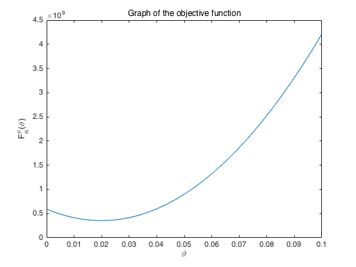
The simulation result is shown in Figure 1, which indicates that our estimator is a good approximation for the true parameter value.

References

- [1] Brettschneider T, Volpe G., Helden L., Wehr J. and Bechinger C.: Force measurement in the presence of Brownian noise: equilibrium-distribution method versus drift method. Physical Review E, 83 (041113), 2011.
- [2] Duan J.: An Introduction to Stochastic Dynamics. Cambridge University Press, 2015.
- [3] Freidlin M.: Some remarks on the Smoluchowski–Kramers approximation. Journal of Statistical Physics, 117(314):617-634, 2004.
- [4] Hottovy S., Volpe G. and Wehr J.: Noise-induced drift in stochastic differential equations with arbitrary friction and diffusion in the Smoluchowski-Kramers limit. Journal of Statistical Physics, 146, 762-773, 2012.
- [5] Hottovy S., McDaniel A., Volpe G. and Wehr J.: The Smoluchowski-Kramers limit of stochastic differential equations with arbitrary state-dependent friction. Communications in Mathematical Physics, 3 (336), 2015.
- [6] Kasonga R.A.: The consistency of a nonlinear least squares estimator from diffusion processes. Stochastic Processes and their Applications, 30, 263-275, 1988.
- [7] Kramers H. A.: Brownian motion in a field of force and the diffusion model of chemical reactions. Physica, 7, 284–304, 1940.
- [8] Maso G.D.: An Introduction to Convergence. Birkhuser Boston, 1993.
- [9] Nelson E.: Dynamical Theories of Brownian Motion. Princeton University Press, second edition,1967.
- [10] Papanicolaou A: Filtering for fast mean-reverting processes. Asymptotic analysis, 70, 2010.
- [11] Sinha P., Szilagyi I., Ruiz-Cabello F., Maroni P., and Borkovec M.: Attractive forces between charged colloidal particles induced by multivalent ions revealed by confronting aggregation and direct force measurements. The Journal of Physical Chemistry Letters, 4, 648-652, 2013.
- [12] Smoluchowski M.: Drei Vortrge ber diffusion Brownsche Bewegung and Koagulation von Kolloidteilchen. Physik Z, 17, 557-585, 1916.
- [13] Volpe G., Helden L., Brettschneider T., Wehr J., and Bechinger C.: Influence of noise on force measurements. Physical Peview Letters, 104 (170602), 2010.