A Discontinuous Galerkin Fast Spectral Method for the Full Boltzmann Equation
with General Collision Kernels
Abstract
The Boltzmann equation, an integro-differential equation for the molecular distribution function in the physical and velocity phase space, governs the fluid flow behavior at a wide range of physical conditions, including compressible, turbulent, as well as flows involving further physics such as non-equilibrium internal energy exchange and chemical reactions. Despite its wide applicability, deterministic solution of the Boltzmann equation presents a huge computational challenge, and often the collision operator is simplified for practical reasons. In this work, we introduce a highly accurate deterministic method for the full Boltzmann equation which couples the Runge-Kutta discontinuous Galerkin (RKDG) discretization in time and physical space (Su et al., Comp. Fluids, 109 pp. 123-136, 2015) and the recently developed fast Fourier spectral method in velocity space (Gamba et al., SIAM J. Sci. Comput., 39 pp. B658–B674, 2017). The novelty of this approach encompasses three aspects: first, the fast spectral method for the collision operator applies to general collision kernels with little or no practical limitations, and in order to adapt to the spatial discretization, we propose here a singular-value-decomposition based algorithm to further reduce the cost in evaluating the collision term; second, the DG formulation employed has high order of accuracy at element-level, and has shown to be more efficient than the finite volume method; thirdly, the element-local compact nature of DG as well as our collision algorithm is amenable to effective parallelization on massively parallel architectures. The solver has been verified against analytical Bobylev-Krook-Wu solution. Further, the standard benchmark test cases of rarefied Fourier heat transfer, Couette flow, oscillatory Couette flow, normal shock wave, lid-driven cavity flow, and thermally driven cavity flow have been studied and their results are compared against direct simulation Monte Carlo (DSMC) solutions with equivalent molecular collision models or published deterministic solutions.
Keywords:
rarefied gas dynamics , the full Boltzmann equation , deterministic solver , discontinuous Galerkin method , fast Fourier spectral method.2010 MSC
76P05 , 82B40 , 82C40 , 82D05 , 35Q20 , 65T50 , 65M60 , 65M70 , 65Y05References
- [1] W. Su, A. A. Alexeenko, G. Cai, A parallel Runge–Kutta discontinuous Galerkin solver for rarefied gas flows based on 2D Boltzmann kinetic equations, Computers & Fluids 109 (2015) 123–136.
- [2] I. Gamba, J. Haack, C. Hauck, J. Hu, A fast spectral method for the Boltzmann collision operator with general collision kernels, SIAM J. Sci. Comput. 39 (2017) B658–B674.
- [3] Y. Sone, Kinetic theory and fluid dynamics, Springer Science & Business Media, 2002.
- [4] G. Karniadakis, A. Beskok, N. Aluru, Microflows and nanoflows: fundamentals and simulation, vol. 29, Springer Science & Business Media, 2006.
- [5] G. A. Bird, Molecular Gas Dynamics and the Direct Simulation of Gas Flows, Clarendon Press, Oxford, 1994.
- [6] H. Grad, On the kinetic theory of rarefied gases, Communications on pure and applied mathematics 2 (4) (1949) 331–407.
- [7] G. Bird, Approach to translational equilibrium in a rigid sphere gas, The Physics of Fluids 6 (10) (1963) 1518–1519.
- [8] G. Bird, The DSMC method, CreateSpace Independent Publishing Platform, 2013.
- [9] M. A. Gallis, J. Torczynski, D. Rader, G. A. Bird, Convergence behavior of a new DSMC algorithm, Journal of Computational Physics 228 (12) (2009) 4532–4548.
- [10] Q. Sun, I. D. Boyd, G. V. Candler, A. D. Ketsdever, E. Muntz, A Hybrid Continuum/Particle Approach for Micro-Scale Gas Flows, in: AIP Conference Proceedings, vol. 663, AIP, 752–759, 2003.
- [11] G. Dimarco, L. Pareschi, Hybrid multiscale methods II. Kinetic equations, Multiscale Modeling & Simulation 6 (4) (2008) 1169–1197.
- [12] L. L. Baker, N. G. Hadjiconstantinou, Variance reduction for Monte Carlo solutions of the Boltzmann equation, Physics of Fluids 17 (5) (2005) 051703.
- [13] S. K. Stefanov, On DSMC calculations of rarefied gas flows with small number of particles in cells, SIAM Journal on Scientific Computing 33 (2) (2011) 677–702.
- [14] A. Alexeenko, S. Gimelshein, Direct simulation Monte Carlo, in: R. Jonhson (Ed.), The Handbook of Fluid Dynamics, CRC Press Boca Raton, FL, 39:1–40, 2016.
- [15] W. Wagner, A convergence proof for Bird’s direct simulation Monte Carlo method for the Boltzmann equation, Journal of Statistical Physics 66 (3) (1992) 1011–1044.
- [16] E. P. Gross, E. A. Jackson, Kinetic models and the linearized Boltzmann equation, The physics of fluids 2 (4) (1959) 432–441.
- [17] P. L. Bhatnagar, E. P. Gross, M. Krook, A model for collision processes in gases. I. Small amplitude processes in charged and neutral one-component systems, Physical review 94 (3) (1954) 511.
- [18] L. H. Holway Jr, New statistical models for kinetic theory: methods of construction, Physics of Fluids (1958-1988) 9 (9) (1966) 1658–1673.
- [19] M. A. Gallis, J. R. Torczynski, S. J. Plimpton, D. J. Rader, T. Koehler, J. Fan, Direct simulation Monte Carlo: The quest for speed, in: AIP Conference Proceedings, vol. 1628, AIP, 27–36, 2014.
- [20] M. Gallis, J. Torczynski, D. Rader, M. Tij, A. Santos, Normal solutions of the Boltzmann equation for highly nonequilibrium Fourier flow and Couette flow, Physics of Fluids 18 (1) (2006) 017104.
- [21] C. D. Levermore, Moment closure hierarchies for kinetic theories, Journal of statistical Physics 83 (5-6) (1996) 1021–1065.
- [22] H. Struchtrup, M. Torrilhon, Regularization of Grad’s 13 moment equations: derivation and linear analysis, Physics of Fluids 15 (9) (2003) 2668–2680.
- [23] X.-j. Gu, D. R. Emerson, A high-order moment approach for capturing non-equilibrium phenomena in the transition regime, Journal of fluid mechanics 636 (2009) 177–216.
- [24] Z. Cai, Y. Fan, R. Li, Globally hyperbolic regularization of Grad’s moment system, Communications on pure and applied mathematics 67 (2014) 464–518.
- [25] L. Mieussens, A survey of deterministic solvers for rarefied flows, in: Proceedings of the 29th International Symposium on Rarefied Gas Dynamics, AIP Conf. Proc, vol. 1628, 943–951, 2014.
- [26] G. Dimarco, L. Pareschi, Numerical methods for kinetic equations, Acta Numer. 23 (2014) 369–520.
- [27] L. Pareschi, G. Russo, Numerical solution of the Boltzmann equation I: spectrally accurate approximation of the collision operator, SIAM J. Numer. Anal. 37 (2000) 1217–1245.
- [28] I. M. Gamba, S. H. Tharkabhushanam, Spectral-Lagrangian methods for collisional models of non-equilibrium statistical states, J. Comput. Phys. 228 (2009) 2012–2036.
- [29] C. Mouhot, L. Pareschi, Fast algorithms for computing the Boltzmann collision operator, Math. Comp. 75 (2006) 1833–1852.
- [30] L. Wu, C. White, T. J. Scanlon, J. M. Reese, Y. Zhang, Deterministic numerical solutions of the Boltzmann equation using the fast spectral method, Journal of Computational Physics 250 (2013) 27–52.
- [31] L. Wu, J. Reese, Y. Zhang, Solving the Boltzmann equation determinstically by the fast spectral method: application to gas microflows, Journal of Fluid Mechanics 746 (2014) 52–84.
- [32] L. Wu, H. Liu, Y. Zhang, J. M. Reese, Influence of intermolecular potentials on rarefied gas flows: Fast spectral solutions of the Boltzmann equation, Physics of Fluids 27 (8) (2015) 082002.
- [33] B. Cockburn, C.-W. Shu, TVB Runge-Kutta local projection discontinuous Galerkin finite element method for conservation laws. II. General framework, Mathematics of computation 52 (186) (1989) 411–435.
- [34] B. Cockburn, S.-Y. Lin, C.-W. Shu, TVB Runge-Kutta local projection discontinuous Galerkin finite element method for conservation laws III: one-dimensional systems, Journal of Computational Physics 84 (1) (1989) 90–113.
- [35] B. Cockburn, C.-W. Shu, The Runge–Kutta discontinuous Galerkin method for conservation laws V: multidimensional systems, Journal of Computational Physics 141 (2) (1998) 199–224.
- [36] B. Cockburn, S. Hou, C.-W. Shu, The Runge-Kutta local projection discontinuous Galerkin finite element method for conservation laws. IV. The multidimensional case, Mathematics of Computation 54 (190) (1990) 545–581.
- [37] J. S. Hesthaven, T. Warburton, Nodal Discontinuous Galerkin Methods: Algorithms, Analysis, and Applications, Springer Science & Business Media, 2007.
- [38] A. Alexeenko, C. Galitzine, A. Alekseenko, High-order discontinuous Galerkin method for Boltzmann model equations, in: 40th Thermophysics Conference, 4256, 2008.
- [39] W. Su, Z. Tang, B. He, G. Cai, Stable Runge-Kutta discontinuous Galerkin solver for hypersonic rarefied gaseous flow based on 2D Boltzmann kinetic model equations, Applied Mathematics and Mechanics 38 (3) (2017) 343–362.
- [40] T. Barth, On discontinuous Galerkin approximations of Boltzmann moment systems with Levermore closure, Computer methods in applied mechanics and engineering 195 (25-28) (2006) 3311–3330.
- [41] M. Abdelmalik, E. van Brummelen, An entropy stable discontinuous Galerkin finite-element moment method for the Boltzmann equation, Computers & Mathematics with Applications 72 (8) (2016) 1988–1999.
- [42] C. Cercignani, The Boltzmann Equation and Its Applications, Springer-Verlag, New York, 1988.
- [43] A. L. Fetter, J. D. Walecka, Theoretical Mechanics of Particles and Continua, Dover Publications, 2012.
- [44] K. Koura, H. Matsumoto, Variable soft sphere molecular model for inverse-power-law or Lennard-Jones potential, Physics of fluids A: fluid dynamics 3 (10) (1991) 2459–2465.
- [45] A. B. Weaver, A. A. Alexeenko, Revised variable soft sphere and Lennard-Jones model parameters for eight common gases up to 2200 K, Journal of Physical and Chemical Reference Data 44 (2) (2015) 023103.
- [46] K. Swaminathan-Gopalan, K. A. Stephani, Recommended direct simulation Monte Carlo collision model parameters for modeling ionized air transport processes, Physics of Fluids 28 (2) (2016) 027101.
- [47] A. Venkattraman, A. A. Alexeenko, Binary scattering model for Lennard-Jones potential: Transport coefficients and collision integrals for non-equilibrium gas flow simulations, Physics of Fluids 24 (2) (2012) 027101.
- [48] G. Karniadakis, S. Sherwin, Spectral/hp element methods for CFD, 1999.
- [49] S. Gottlieb, D. Ketcheson, C.-W. Shu, Strong Stability Preserving Runge-Kutta and Multistep Time Discretizations, World Scientific, 2011.
- [50] L. Mieussens, Discrete-velocity models and numerical schemes for the Boltzmann-BGK equation in plane and axisymmetric geometries, Journal of Computational Physics 162 (2) (2000) 429–466.
- [51] A. Bobylev, Exact solutions of the Boltzmann equation, in: Akademiia Nauk SSSR Doklady, vol. 225, 1296–1299, 1975.
- [52] M. Krook, T. T. Wu, Exact solutions of the Boltzmann equation, The Physics of Fluids 20 (10) (1977) 1589–1595.
- [53] M. A. Gallis, N. P. Bitter, T. P. Koehler, J. R. Torczynski, S. J. Plimpton, G. Papadakis, Molecular-Level Simulations of Turbulence and its Decay 118 (6) (2017) 064501.
- [54] M. A. Gallis, T. P. Koehler, J. R. Torczynski, S. J. Plimpton, Direct simulation monte carlo investigation of the Rayleigh-Taylor instability 1 (4) (2016) 043403.
- [55] C. Pekardan, A. Alexeenko, Rarefaction effects for the transonic airfoils in low Reynolds number regime, in: 46th AIAA Thermophysics Conference, 4429, 2016.
- [56] I. B. Sebastiao, L. Qiao, A. A. Alexeenko, Direct Simulation Monte Carlo Modeling of H2-O2 Deflagration Waves 198 (2018) 40–53.
- [57] M. Gallis, D. Rader, J. Torczynski, Calculations of the near-wall thermophoretic force in rarefied gas flow, Physics of Fluids 14 (12) (2002) 4290–4301.
- [58] C. R. Lilley, J. E. Sader, Velocity gradient singularity and structure of the velocity profile in the Knudsen layer according to the Boltzmann equation, Physical Review E 76 (2) (2007) 026315.
- [59] T. Ohwada, Structure of normal shock waves: Direct numerical analysis of the Boltzmann equation for hard-sphere molecules, Physics of Fluids A: Fluid Dynamics 5 (1) (1993) 217–234.
- [60] B. John, X.-J. Gu, D. R. Emerson, Investigation of heat and mass transfer in a lid-driven cavity under nonequilibrium flow conditions, Numerical Heat Transfer, Part B: Fundamentals 58 (5) (2010) 287–303.
- [61] M. Kogan, V. Galkin, O. Fridlender, Stresses produced in gases by temperature and concentration inhomogeneities. New types of free convection, Usp. Fiz. Nauk 119 (1976) 111–125.
- [62] R. Womersley, Symmetric Spherical Designs on the sphere with good geometric properties, The University of New South Wales. URL http://web.maths.unsw.edu.au/$\sim$rsw/Sphere/EffSphDes/ss.html.
- [63] C. H. L. Beentjes, Quadrature on a spherical surface, Tech. Rep., University of Oxford, 2015.
1 Introduction
In micro/rarefied gas flows, the gas molecule wall-surface interactions lead to the formation of Knudsen layer (KL): a local thermodynamically non-equilibrium region extending from the surface, where is the gas mean free path (MFP) Sone [2002]. The Knudsen number () is defined as , where is the characteristic length of the system. The classical constitutive relations of the Navier-Stokes-Fourier equations fail to predict nonlinear behavior in the KL and deviations are significant in the slip () and transition flow regimes () Sone [2002], Karniadakis et al. [2006], Bird [1994]. The Boltzmann equation, an integro-differential equation for the molecular distribution function in the physical and velocity phase space, governs the fluid flow behavior for a wide range of Knudsen numbers and physical conditions, including compressible, turbulent, as well as flows involving further physics such as non-equilibrium internal energy exchange and chemical reactions. Accurate physical models and efficient numerical methods are required for solving the Boltzmann equation so as to predict the non-equilibrium phenomenon encountered in such rarefied flows.
The approaches for numerical solution of the Boltzmann equation date back to as early as 1940s Grad [1949] using, for example, the now widely used direct simulation Monte Carlo (DSMC) method Bird [1963], Bird [2013]. The DSMC method, based on the kinetic theory of dilute gases, models the binary interactions between particles stochastically. However, it is this stochastic nature of the method that introduces high statistical noise in low-speed flows, and imposes strict constraints on cell-size and time-step. Moreover, the formal accuracy of particle time-stepping is linear. The stiffness properties of the Boltzmann equation further aggravates the time-step constraints. To overcome these limitations, improved particle-based approaches have been proposed Gallis et al. [2009], including hybrid continuum/particle solvers Sun et al. [2003], Dimarco and Pareschi [2008], variance reduction methods Baker and Hadjiconstantinou [2005], and simplified Bernoulli trials Stefanov [2011].
It is to be noted that the assertion that DSMC solves the actual full Boltzmann equation is not strictly valid. Indeed, the DSMC method can be derived rigorously as the Monte Carlo solution of the -particle master kinetic equation Alexeenko and Gimelshein [2016]. Wagner Wagner [1992] established convergence proof for Bird’s DSMC method for the Boltzmann equation in the limit of infinite number of particles, . Moreover, the proof has inherent assumptions on the boundedness of the collision operator which is clearly highlighted in Wagner’s work (see section 5 in Wagner [1992]).
The deterministic solutions based on discretization of governing differential equations on representative grids is central to computational fluid dynamics (CFD). However, the multi-dimensional nature of the Boltzmann equation and the collision integral becomes a bottleneck resulting in excessive use of time and computing resources. To bypass this issue, simplified Boltzmann equation variants such as linearized Boltzmann (LB) Gross and Jackson [1959], Bhatnagar-Gross-Krook (BGK) Bhatnagar et al. [1954], and ellipsoidal Bhatnagar-Gross-Krook (ES-BGK) Holway Jr [1966] equations are used. These simplified models perform better at low Knudsen number flows in slip and early transition regimes. Yet they often fail to capture the physics at high Knudsen numbers as well as for diffusion dominated flows at even low Knudsen numbers (see Gallis et al. [2014], Gallis et al. [2006]). Another way to reduce the dimensionality is to consider the moment closure of the Boltzmann equation. Introduced by Grad Grad [1949], the moment method produces an evolution equation for the moments of the distribution function. Different level of approximations/closures lead to different hierarchies, e.g., Grad 13-moment Grad [1949], Levermore 14-moment Levermore [1996], and various regularized versions Struchtrup and Torrilhon [2003], Gu and Emerson [2009], Cai et al. [2014].
Over the past decades, the deterministic methods that solve the full Boltzmann equation have undergone considerable development. Without being exhaustive, we refer to Mieussens [2014], Dimarco and Pareschi [2014] for a comprehensive review. In this work, we employ the recently developed fast Fourier spectral method Gamba et al. [2017] to solve the Boltzmann collision operator. Compared with other deterministic methods such as the discrete velocity models (DVM), the Fourier spectral method can provide significantly more accurate results with less numerical complexity; compared with DSMC, it produces smooth, noise-free solutions and can simulate low-speed flows such as those encountered often in micro-systems. On the other hand, the Fourier spectral method is still computationally demanding, as it requires memory to store precomputed weights and has numerical complexity Pareschi and Russo [2000], Gamba and Tharkabhushanam [2009], where is the number of discretization points in each velocity dimension. The main contribution in Gamba et al. [2017] is a low-rank strategy to accelerate the direct Fourier spectral method so that it requires only memory to store precomputed weights (no precomputation is needed in certain cases) and has complexity, where is the number of discretization points on the sphere and . Furthermore, the fast method applies directly to arbitrary collision kernels and can be easily extended to general collision models including the multi-species and inelastic Boltzmann equations. We mention that there is another line of research that develops the fast Fourier spectral method based on Carleman representation of the collision operator Mouhot and Pareschi [2006]. The complexity of the method is . However, its applicability is limited to hard sphere molecules. The method has been extended to anisotropic scattering in Wu et al. [2013], but it assumes a special form of the kernel and requires recalibration of transport coefficients and parametric fitting therein. This methodology has been applied to Lennard-Jones potential and to many canonical flows in Wu et al. [2014],Wu et al. [2015]. The method has been extended to anisotropic scattering in Wu et al. [2013] and applied to many canonical flows in Wu et al. [2014] by assuming a special form of the kernel and performing a recalibration of transport coefficients and parametric fitting. In Wu et al. [2015], the Lennard-Jones potential was considered by fully resolving the kernel, resulting in the cost of .
All of the former approaches have relied on low-order (up to second-order) finite volume (FV) or finite difference (FD) methods for spatial discretization of the Boltzmann equation. In this work, we employ the discontinuous Galerkin (DG) method for the spatial discretization, a class of high order method widely used for time dependent multi-dimensional hyperbolic equations Cockburn and Shu [1989], Cockburn et al. [1989], Cockburn and Shu [1998], Cockburn et al. [1990], Hesthaven and Warburton [2007]. Compared to high-order FV/FD methods, DG provides easy formulation on arbitrary meshes, high-order flux reconstruction, straightforward implementation of boundary conditions, high-order accuracy, as well as strong linear scaling on parallel processors due to the compactness of the scheme Hesthaven and Warburton [2007]. DG has been employed for solving the BGK and ES-BGK equations for 0D/1D Alexeenko et al. [2008], and 2D Su et al. [2015], Su et al. [2017] flow problems. It has also been used to approximate the moment systems of the Boltzmann equation in Barth [2006], Abdelmalik and van Brummelen [2016]. To the best of our knowledge, DG discretization in the physical space hasn’t been applied for solving the full Boltzmann equation till date.
To summarize, we present a 1D/2D-3V full Boltzmann equation solver by coupling the Runge-Kutta discontinuous Galerkin (RKDG) discretization in time and physical space Su et al. [2015] and the fast Fourier spectral method in velocity space Gamba et al. [2017]. The method is high order in both physical space and time, and spectrally accurate in velocity space. There are no ad-hoc adjustments or parametric fitting involved in our present formulation for solving the collision operator. Moreover, our singular value decomposition (SVD) variant of the algorithm for evaluating weak form of the collision term is novel and unique to DG formulation.
In the section that follows, we give a brief introduction of the Boltzmann equation and the collision kernel involved. Section 3 presents an overview of the DG method in general, and describes the weak DG formulation of the Boltzmann equation, including the direct and SVD variant of the algorithm for evaluating the collision term. Extensive numerical experiments and results are performed and discussed in Section 4. Concluding remarks are given in Section 5. A brief description of the fast Fourier spectral method is provided in the Appendix.
2 The Boltzmann equation
The Boltzmann equation for a single-species, monatomic gas without external forces can be written as (cf. Cercignani [1988])
| (1) |
where is the one-particle distribution function of time , position , and particle velocity . gives the number of particles to be found in an infinitesimal volume centered at the point of the phase space. is the collision operator describing the binary collisions among particles, and acts only in the velocity space:
| (2) |
where and denote the pre- and post- collision velocity pairs, which are related through momentum and energy conservation as
| (3) |
with the vector varying over the unit sphere . The quantity () is the collision kernel depending only on and the scattering angle (angle between and ), and can be expressed as
| (4) |
Given the interaction potential between particles, the specific form of can be determined using the classical scattering theory (cf. Fetter and Walecka [2012]):
| (5) |
where is the differential cross-section given by
| (6) |
with being the impact parameter.
With a few exceptions (e.g. hard sphere molecules), the explicit form of can be hard to obtain since is related to implicitly. To avoid this complexity, phenomenological collision kernels are often used in practice with the aim to reproduce the correct transport coefficients. Koura et al. Koura and Matsumoto [1991] introduced a scattering model so called as variable soft sphere (VSS) by assuming an explicit cosine dependence between the scattering angle and impact parameter:
| (7) |
where is the scattering parameter, and is the diameter borrowed from Bird’s Bird [1994] variable hard sphere (VHS) model:
| (8) |
Here is the gas constant ( is the Boltzmann’s constant and is the single particle mass), denotes the usual Gamma function, , , and are, respectively, the reference diameter, reference temperature, and viscosity index. The diameter and exponent are determined so that the transport (viscosity and diffusion) coefficients of VSS are consistent with experimental data Weaver and Alexeenko [2015], Swaminathan-Gopalan and Stephani [2016].
Substituting (7), (8) into (6) and (5), we obtain the general form of as
| (9) |
where is a constant given by
| (10) |
In particular, the VHS kernel is obtained when and ( corresponds to the Maxwell molecules, and , to the hard spheres); and the VSS kernel is obtained when and .
It is worth emphasizing that although the collision kernel (9) is adopted in the present work for easy comparison with DSMC solutions, the fast spectral method we use for the collision operator applies straightforwardly to any kernel of the form (4), i.e., can be any function of the relative velocity and scattering angle as long as the collision integral makes sense (see Appendix). This generality allows us to treat many well studied/calibrated collision models in the existing literature, for example, for Lennard-Jones interactions, one can use the tabulated kernel as obtained in Venkattraman and Alexeenko [2012].
Given the distribution function , the macroscopic quantities can be obtained via its moments:
| (11) |
where , , , , and are, respectively, the number density, bulk velocity, temperature, stress tensor, and heat flux vector.
2.1 Non-dimensionalization
To reduce the parameters, it is convenient to non-dimensionalize all variables and functions.
We first choose the characteristic length , characteristic temperature , and characteristic number density , and then define the characteristic velocity and characteristic time .
Now we rescale , , , and as follows
| (12) |
the macroscopic quantities as
| (13) |
and the collision kernel as
| (14) |
then the equation (1) becomes
| (15) |
with the collision operator
| (16) |
where
| (17) |
The Knudsen number is given by
| (18) |
which is the ratio between the MFP and characteristic length (consistent to equation (4.65) in Bird [1994], Bird [2013]). Finally, the definition (11) in rescaled variables reduces to
| (19) |
3 Discontinuous Galerkin formulation
3.1 Brief overview
The Runge Kutta discontinuous Galerkin (RKDG) method Cockburn and Shu [1989], Cockburn et al. [1989], Cockburn and Shu [1998], Cockburn et al. [1990], Hesthaven and Warburton [2007] is a class of finite element methods coupling RK discretization in time and DG discretization in space which provides high-order numerically accurate solutions to governing partial differential equations. Higher order accuracy is desirable for simulating flows with strong gradients, droplet collisions as in multi-phase flows, combustion-modeling, reactors, and micro-mechanical systems. RKDG can recover flow properties at the domain boundaries with the same high-order accuracy as in the interior of the domain.
In the Boltzmann equation simulations, the computational domain consists of physical and velocity domains. We propose to use the RKDG method in time and physical space and the Fourier spectral method in the velocity space. Hence the velocity space is partitioned using the Cartesian type grid point (with reasons to be explained in section 3.3), and the physical space is split up into a set of line segments (in 1D), triangles/quadrilaterals (in 2D), and tetrahedrals/prisms/hexahedrals (in 3D) for instance. In particular for 2D grids of quadrilateral cells, each cell in the physical space has four faces. The cell connectivity is such that a cell face is either internal and intersects two cells only, or comprises part of an external boundary and belongs to single cell only.
In such a grid system, the DG method is developed to solve the Boltzmann equation at each velocity grid point . Within a given spatial element , the distribution function is approximated as a linear combination of orthogonal basis functions as
| (20) |
where is the number of unknowns in the element also known as local degree of freedom. The task is to determine the coefficients of the expansion for all elements. Therefore, the complexity of the problem is proportional to the number of velocity nodes, the number of spatial elements, the order of basis functions, and the number of time integration steps. Due to the multi-dimensionality of the problem, and the typical size of phase space considered in the current work (order of millions), parallel computation is highly desirable.
In finite element setting, the information is exchanged between two-adjacent elements using the shared nodes between them. The DG method, in contrast to the classical finite element method that relies on global stiffness matrices, duplicates the values that are shared between the elements. To connect the elements at the shared nodes, DG introduces monotone interface flux (as in finite volume method). It is this flux that allows element-to-element decoupling, recovers a meaningful global solution, and allows for explicit time stepping (see Hesthaven and Warburton [2007]). It is this element-to-element decoupling and element local-nature of the DG method that makes it amenable to strong scaling on parallel processors, and therefore our choice of spatial discretization scheme.
3.2 Discretization in the physical space
Assume that the Boltzmann equation (15) is posed in the domain with boundary in the physical space. We decompose into variable sized elements :
| (21) |
In each element , we approximate the function by a polynomial of order :
| (22) |
where is the basis function supported in , is the total number of terms in the local expansion, and is the elemental degree of freedom. In general depends on elemental-shape. In 1D, . In 2D, for quadrilateral elements, and for triangular elements. In 3D, for hexahedral elements, and for tetrahedral elements.
We now present a general 3D spatial weak DG formulation for the Boltzmann equation. Reduction to the 2D case can be achieved by choosing a 2D basis, and ignoring the -axis dependence. Similarly for the 1D case. Time and velocity space are left as continuous at the moment.
We first form the residual by substituting the expansion (22) into the equation (15):
| (23) |
where we used the quadratic nonlinearity of the collision operator.
We then require that the residual is orthogonal to all test functions. In the Galerkin formulation, the test function is the same as the basis function, thus
| (24) |
in each element .
Substituting (23) into (24) and applying the divergence theorem, we obtain
| (25) |
where is the local outward pointing normal and denotes the numerical flux. Specifically, the surface integral in the above equation is defined as follows
| (26) |
with and being the outward normal and numerical flux along the face . In our implementation, we choose the upwind flux:
| (27) |
where int and ext denote interior and exterior of the face respectively.
Note that the second term in equation (25) can be expanded as
| (28) |
where , , are the three components of .
3.3 Discretization in the velocity space
To further discretize the system (34) in the velocity space, we employ a finite difference (or discrete velocity) discretization. Each velocity component () is discretized uniformly with points in the interval . The grid points are chosen as , with and (the choice of is given below). For brevity we will use to denote the 3D velocity grid point.
The reason of using the uniform velocity grid is because our fast algorithm for the collision operator is based on Fourier transform, which is naturally done on a uniform mesh (see Appendix for details). Simply speaking, it takes the function values at the grid points as input, does the calculation (including forward and backward FFTs) in a black box solver, and outputs the values of the collision operator at the same grid points. Inside the solver, it assumes the distribution function has a compact support, and chooses a relatively large computational domain enclosing this support, then periodically extends the function to the whole space . As such, the method can achieve spectral accuracy (subject to domain truncation error which is usually very small); furthermore, the simple mid-point rule would also allow one to construct the moments with spectral accuracy.
To determine the domain size , we first choose the maximum temperature and velocity specified at all boundaries, and estimate such that the interval defined as
| (35) |
can produce the correct values of and (i.e., it is large enough that the tail truncation effects of the Gaussian characterized by and are negligible). Finally, is chosen as
| (36) |
which is a relatively safe choice to avoid aliasing effect (Pareschi and Russo [2000]). In general, the parameter ranges between 1 to 3.
With the above setup, we just need to solve the system (34) at each velocity grid and in each spatial element .
The macroscopic quantities defined in (19): density, bulk velocity, temperature, stress tensor, and heat flux in the spatial element can be recovered using numerical integration (mid-point rule) of the distribution function over the entire velocity grid:
| (37) |
where . Note that , , , , are polynomials defined in each element since are polynomials.
3.3.1 Evaluation of the collision term
We are now left with the issue of evaluating the collision term in (34):
| (38) |
Note here that the collision operator acts only in the velocity variable .
The method we use was proposed in Gamba et al. [2017]. Given a function at velocity grid, it produces at the same grid with complexity, where is the number of quadrature points on the sphere and . In the Appendix, we give a brief description of this method for evaluating the operator of the form with general collision kernel (4). Compared to the original method in Gamba et al. [2017], we improve the accuracy and efficiency by using a different quadrature on the half sphere.
Equipped with the fast collision solver, the complexity of evaluating (38) would be for all , where the first term is to generate for all and , and the second term is to evaluate the outer double summation. For (relatively) high-order polynomial approximations, can be large. To further reduce the cost, here we propose a simple approach based on singular value decomposition (SVD).
For each fixed m (), we precompute the SVD of the matrix as
| (39) |
where is the rank of the matrix and (the diagonal matrix in the usual SVD has been absorbed in the term in the above notation). Substituting (39) into (38) yields
| (40) |
Note that the functions and can be computed in a different loop. Therefore, the complexity of evaluating (38) becomes . For the conventional nodal DG basis Karniadakis and Sherwin [1999], Hesthaven and Warburton [2007] used in the current work, we found that for many , can be much smaller than , thus is strictly less than . Comparing with the aforementioned direct method, we can see that the SVD approach always saves. Considering that the evaluation of the collision operator always constitutes the main bottleneck in the computation, this saving, may not be in the order of magnitude, is still appreciable.
We mention that the rank of the matrix strongly depends on the underlying DG basis. The structure of for various element shapes is currently under study and will be reported in future work.
3.4 Discretization in time
Once the spatial and velocity discretization is done, the time discretization can be performed by simply applying an explicit Runge-Kutta method to the system (34). Here we adopt the widely used strong-stability-preserving (SSP) RK schemes Gottlieb et al. [2011].
For notational simplicity, we rewrite the system (34) as
| (41) |
and use to denote the solution vector with components , .
Then the 2nd order SSP-RK scheme is given by
and the 3rd order SSP-RK scheme is given by
3.5 Initial and boundary conditions
The initial value of the distribution function is set to Maxwellian at given initial macroscopic conditions , , and :
| (47) |
For the test cases considered in the current work, the fully diffusive Maxwell boundary condition is assumed at the wall Mieussens [2000] except the normal shock wave example in Section 4.7. Consider a wall moving with velocity , and is at temperature , the inflow boundary condition at with the local outward pointing normal is given by
| (48) |
with
| (49) |
and is determined from conservation of mass as
| (50) |
For the normal shock wave example, we use the inflow boundary condition at :
| (51) |
where , , are the prescribed inlet conditions. Details about other boundary conditions can be found in Bird [1994], Cercignani [1988], Su et al. [2015].
4 Numerical experiments and results
In this section, we evaluate the accuracy of the proposed discontinuous Galerkin fast spectral method, which we shall denote by the acronym DGFS in the following. A nodal DG basis has been used similar to the ones described in Karniadakis and Sherwin [1999], Hesthaven and Warburton [2007].
Standard benchmark cases of Bobylev-Krook-Wu (BKW) solution Bobylev [1975], Krook and Wu [1977], planar Fourier heat transfer, Couette flow, oscillatory Couette flow, normal shock, lid driven cavity flow, and thermally driven cavity flow have been considered in the present work. The results are compared with those obtained from the DSMC method Bird [1994] with equivalent molecular collision models, analytical solution, or published deterministic solutions, wherever applicable.
4.1 Solver configurations
SPARTA Gallis et al. [2014] has been employed for carrying out DSMC verifications in the present work. It implements the DSMC method as proposed by Bird Bird [1994]. The solver has been benchmarked Gallis et al. [2014] and widely used for studying hypersonic, subsonic and thermal Gallis et al. [2017], Gallis et al. [2016], Pekardan and Alexeenko [2016], Sebastiao et al. [2018] gas flow problems. In this work, cell size less than has been ensured in all the test cases. A minimum of 30 DSMC simulator particles per cell are used in conjunction with the no-time collision (NTC) algorithm. Each steady-state simulation has been averaged for a minimum 100,000 steps so as to minimize the statistical noise.
Our numerical tests in this work are restricted to monatomic gases. Argon gas with mass kg, reference viscosity of N/ms at reference temperature of is selected. The molecular diameters are selected so as to maintain the reference viscosity: , for the Maxwell collision model, and , for the VHS collision model. These values are consistent for both DSMC and DGFS in all test cases unless otherwise explicitly stated.
In rarefied gas dynamics, two widely used definitions of Knudsen number exist. The first definition is by Cercignani Cercignani [1988], the second definition is by Bird Bird [1994] (i.e. the equation (18) in the present work). Here we want to compare our results with DSMC results published in the literature, for instance, Fourier heat transfer in Gallis at al. Gallis et al. [2002], Couette flow in Gu et al. Gu and Emerson [2009]. These works use Cercignani’s definition. Therefore, for consistency, the Knudsen number defined in this section follows Cercignani’s definition, i.e., , where and is the dynamic viscosity. Using Bird’s power law for viscosity, the ratio of these two Knudsen numbers is simply a constant given by
| (52) |
4.2 Hardware configurations
MPI-parallel implementation of DSMC solver (SPARTA) is run on Intel E5-2680 Xeon(TM) Processor v2 2.80 GHz (Conte cluster at Purdue). The operating system used is 64-bit RHEL 6.7. The solver has been written in C++ and is compiled using OpenMPI mpic++ 1.8.1, g++ 5.2.0 with OpenMP-4.0 support, and third level optimization flags.GPU-parallelized implementations of DGFS solver are run on Intel Xeon E5 2623 v4 2.60 GHz CPU with NVIDIA Titan-X (Pascal) GPU accompanying CUDA driver 8.0 and CUDA runtime 8.0. The operating system used is 64-bit Red Hat 6.9 (Santiago). The GPU has 5376 CUDA cores, 12GB device memory, and compute capability of 6.1. The solver has been written in C++/CUDA and is compiled using g++ 5.3.0, and nvcc 8.0.44 compiler with third level optimization flag. All the simulations are done with double precision floating point values.
4.3 0D case: BKW solution
For constant collision kernel , an analytical solution to the spatially homogeneous Boltzmann equation
| (53) |
can be constructed as (see Bobylev [1975], Krook and Wu [1977])
| (54) |
where . Upon differentiation, one recovers the exact as
| (55) |
where . The initial time must be greater than for to be positive. An arbitrary time of has been picked in the present work. The 3rd order SSP-RK scheme (3.4) with is employed for time integration. Velocity domain size has been used for the present case.
4.3.1 Error in evaluation of the collision operator
Using (55), one can verify the accuracy of the proposed method without introducing additional time discretization error. Table 1 shows the error in evaluating the collision operator i.e., . As noted in the Appendix, the total number of Gauss-Legendre quadrature points in the radial direction should be on order of . As per Gamba et al. [2017], a more precise estimate is . However, there is no good rule to select optimal . From Table 1, we observe that the error is relatively unaffected upon reducing from to . However, we note that is a safer choice. For all cases considered henceforth, , unless otherwise explicitly stated.
| 8 | 2 | 4.06e-03 | 2.26e-03 | 6.04e-04 |
|---|---|---|---|---|
| 4 | 1.51e-03 | 5.58e-04 | 1.00e-03 | |
| 8 | 1.26e-03 | 6.92e-04 | 1.16e-03 | |
| 16 | 4 | 1.89e-03 | 7.42e-04 | 9.06e-05 |
| 8 | 1.65e-04 | 8.22e-05 | 7.39e-06 | |
| 16 | 1.71e-04 | 8.38e-05 | 6.56e-06 | |
| 24 | 6 | 7.72e-04 | 5.18e-04 | 6.70e-05 |
| 12 | 2.41e-05 | 4.22e-06 | 9.05e-08 | |
| 24 | 2.42e-05 | 4.19e-06 | 9.07e-08 | |
| 32 | 8 | 2.10e-04 | 5.77e-05 | 2.39e-06 |
| 16 | 5.22e-08 | 3.90e-08 | 7.04e-08 | |
| 32 | 5.23e-08 | 3.90e-08 | 7.04e-08 | |
| 48 | 12 | 7.40e-07 | 1.26e-07 | 7.02e-08 |
| 24 | 1.88e-08 | 3.81e-08 | 7.04e-08 | |
| 48 | 1.88e-08 | 3.81e-08 | 7.04e-08 | |
| 64 | 16 | 1.88e-08 | 3.81e-08 | 7.05e-08 |
| 32 | 1.88e-08 | 3.81e-08 | 7.05e-08 | |
| 64 | 1.88e-08 | 3.81e-08 | 7.05e-08 | |
4.3.2 Normalized error
Figure 1 shows the time evolution of normalized error in norm between the numerical and analytical solutions with logarithmic -axis. We have considered the cases , 32, and 64 points in each velocity dimension; and , 16 spherical design quadrature points on the half sphere. A good agreement between analytical and numerical solutions is clearly evident from the figure. It is also observed that the differences between and solutions, i.e. are small (quantitatively on the order of ). The slight increase of the error in the cases of and is due to the aliasing effect of the spectral method as discussed in Pareschi and Russo [2000].
4.3.3 Time evolution of the distribution function
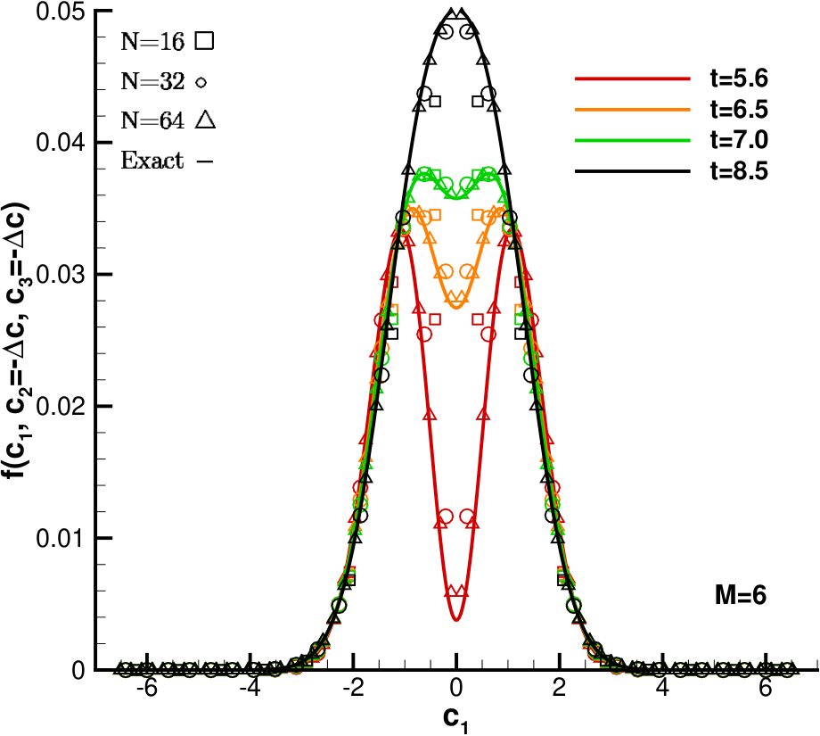
Figure 2 illustrates the time evolution of the distribution function sliced along the velocity domain centerline, i.e., . The smooth analytical solution is plotted by discretizing the velocity space with points. The numerical solution is evaluated by discretizing the velocity space with , and respectively. spherical design quadrature points is used on the half sphere in all cases. It is observed that: a) as increases, the numerical solution moves closer to the smooth analytical solution at different time instants; b) as time goes by, the distribution function tends toward the Maxwellian.
4.3.4 Time evolution of the entropy
The H-theorem states that the entropy is always decreasing (the physical entropy is increasing), which can be expressed mathematically as
| (56) |
where is the so-called H-function or entropy. The entropy can be a powerful quantity for verification of numerical solutions in rarefied flows. Using the mid-point rule, the entropy can be approximated as
| (57) |
The Fourier spectral approximations do not necessarily maintain the positivity of the distribution function. At points where becomes negative, we consider two approaches: (a) evaluate the entropy using the absolute value , or (b) ignore the contribution of these points in the entropy. Figure 3(a) illustrates the time evolution of the analytical entropy and numerical entropy using the approach (a); and Figure 3(b) illustrates the same quantity evaluated using the approach (b). We observe that, in particular, for velocity grid, although the relative error of the distribution function is on the order of as shown in Figure 1, the entropy in this case evaluated using approach (a) is significantly lower than the analytical one, and also qualitatively violates the second law of thermodynamics; the entropy evaluated using approach (b) is not very accurate as well, however, it does predict the correct trend. Hence the second approach is preferable. We believe that this comparison of analytical/numerical entropy is fairly significant for establishing the importance of the fast spectral method.
4.4 1D case: Fourier heat transfer
For the spatially inhomogeneous case, analytical solutions for the Boltzmann equation do not exist. Therefore, we compare our results with DSMC which solves the Boltzmann equation stochastically. In the current test, the coordinates are chosen such that the walls are parallel to the direction and is the direction perpendicular to the walls. The geometry as well as boundary conditions are shown in Figure 4. The two parallel walls, at rest, are set distance apart. The reference (), left-wall (), and right-wall () temperatures are 273K, 263K, and 283K, respectively. The simulation is carried out at three different Knudsen numbers namely , , and by varying the density while keeping the fixed. The 2nd order SSP-RK scheme (3.4) is used for time evolution. Argon with collision model is taken as the working gas (see Gallis et al. [2002] for additional DSMC conditions).
4.4.1 Validation: SVD v.s. direct algorithm
Figure 5 illustrates the temperature profile along the domain length obtained using the SVD and direct variants of the collision algorithm. It is observed that the corresponding two curves are inextricable which verifies that both algorithms evaluate the same Boltzmann collision operator.
4.4.2 Temperature at different Knudsen numbers
Figure 6 illustrate the temperature profile along the domain length for different Knudsen numbers obtained using the SVD variant of the algorithm. The results are compared against the DSMC data Gallis et al. [2014], where our DGFS implementation captures the nonlinear Lilley and Sader [2007] nature of temperature profiles in the near wall region, i.e., the Knudsen layer.
To further highlight the nature of DGFS, we increase the temperature difference between the two walls to i.e., and . Figure 7 illustrates the results for this case. The results for Fourier heat transfer cases suggest that the combination of , , and velocity domain size of suffices. In particular, the use of does not change the result significantly.
From a computation viewpoint, DSMC-SPARTA simulations at , with 500 cells, 30 particles per cell, a time-step of 2e-9 sec, 1 million unsteady time-steps, and 100 million steady time-steps, on 32 CPU processors took 11321.6 sec. These DSMC parameters have been taken from the Gallis et al. Gallis et al. [2002]. The parameters have been selected partially to minimize the statistical fluctuations, and avoid linear time-stepping errors inherent to DSMC simulations. On the other hand, DGFS simulations on a single GPU at , , with 10 elements, 2nd order polynomial, , took 4456.54 sec to achieve , where is the distribution function at timestep. Note that these are representative simulation times for indicating the computational efforts required in DGFS and DSMC for 1-D simulations. A detailed comparison between CPU and GPU performance is subject of future study.
4.5 1D case: steady Couette flow
We now consider the effect of velocity gradient on the solution. The geometry remains the same as in previous case. The left and right parallel walls move with a velocity of , and the reference (), left-wall (), and right-wall () temperatures are set to a constant value of 273K. The simulation is carried out at three different Knudsen numbers namely , , and by varying the density while keeping the fixed. The 2nd order SSP-RK scheme (3.4) is used for time evolution. Argon with collision model is taken as the working gas (see Gu and Emerson [2009] for additional DSMC conditions).
Figure 8 illustrates the velocity along the domain length. The deterministic solution is in excellent agreement with the DSMC solution Gu and Emerson [2009], and again our model captures the nonlinearity in the near-wall region.
To further highlight the nature of DGFS, we increase the velocity difference between the two walls to 1000 Mach=3 i.e., at the left and the right walls respectively. Figure 9 illustrates the results for this case. The results for Couette flow cases suggest that the combination of , , and velocity domain size of suffices for subsonic flows. However, one needs larger velocity domain for supersonic flow problems. We want to emphasize that these parameters are rather derived from heuristics, and it is certainly possible that one can obtain good results with other combinations of , , and velocity-space size. There’s a trade-off between the accuracy and computational cost.
From a computation viewpoint, DSMC-SPARTA simulations at , with 500 cells, 30 particles per cell, a time-step of 2e-9 sec, 1 million unsteady time-steps, and 100 million steady time-steps, on 32 processors took 11206.6 sec. The parameters have been again selected to minimize the statistical fluctuations, and avoid linear time-stepping errors inherent to DSMC simulations. On the other hand, DGFS simulations on a single GPU at , with 10 elements, 2nd order polynomial, , took 4541.98 sec to achieve .
4.6 1D unsteady case: oscillatory Couette flow
To demonstrate the time accuracy of the DGFS, we consider the effect of time varying velocity gradient on the solution. The geometry and flow parameters remain the same as in previous case, except that the left wall is at rest, and the right wall moves with a velocity of , where . The simulation is carried out at . The 2nd order SSP-RK scheme (3.4) with is employed for time integration. Specifically for DSMC simulations, the domain is discretized into 50 cells with 100000 particles per cell (PPC) and the results are averaged for every 1000 () time steps.
Figure 10 depicts the time evolution of velocity along the domain for both DSMC and DGFS results. Since the present case is unsteady, high statistical noise is observed in DSMC solutions. In contrast, DGFS produces a sufficiently smooth solution. Nevertheless, both results are in fair agreement with each other. Further, we observe a high amount of slip () at the left wall since the flow is in transition regime.
An accurate unsteady DSMC result is inherently tricky. We carried out set of simulations by varying PPC, cell-count, and . It is observed that keeping fixed, with decrease in PPC, the sample size decreases and consequently the statistical noise increases as illustrated in Figures 10, 11 and 12, 13. Keeping PPC fixed, with increase in , the sample size increases and consequently the statistical noise decreases, but the simulation lags behind in time as a result of high . These observations are depicted in Figures 12 and 13.
Through Figures 11, 12, 13, we want to emphasize the smooth time accurate results obtained from DGFS, and the well-known stochastic nature of DSMC solutions. In present case, we used as large as 10000 particles per cell for obtaining time accurate results. In large scale simulations, 10000 particles per cell might not be feasible computationally, and hence the results from DSMC would always be inaccurate in those cases.
4.7 1D steady case: normal shock wave
To demonstrate the advantage of high order DGFS approximations, we consider the normal shock wave and compare our solutions with the finite-difference solutions reported in Ohwada [1993]. The numerical parameters are listed in Table 2. Specifically for these cases, since the flow is in early slip regime hence the collision term is stiffer, the method acquires steady-state slowly. A convergence criterion of / has been used. Note in particular that the spatial domain has been discretized with just 4 elements, and 3rd order DG for Mach 1.59 case. Limiters have not been used in the present study. Figure 14 illustrates the variation of normalized density, temperature, and velocity for Ma 1.59 normal shock. Note that the position of the shock wave has been adjusted to the location with the average density as per Ohwada [1993]. Based upon these results, one can infer that DGFS is able to resolve the normal shock with just 4 elements within engineering () accuracy. Note that the discontinuity in the flow profile is the characteristic of the DG method. On increasing the number of elements to 8, the results from Ohwada [1993] match fairly well with DGFS. Similarly, Figure 15 depicts the variation of normalized density, temperature, and velocity for Mach 3 normal shock with 8 elements and 3rd order DG. Again, the Mach 3 shock is captured well using just 8 elements.
| Parameter | Case 01 | Case 02 |
|---|---|---|
| Working Gas | Helium | Helium |
| Mach number | 1.59 | 3.0 |
| Physical space () | ||
| Velocity space | ||
| Spatial elements | 4 | 8 |
| DG order | 3 | 3 |
| Viscosity index: | 0.5 | 0.5 |
| Ref. diameter: () | ||
| Ref. Temperature: () | 273 | 273 |
| Upstream conditions: | ||
| Velocity: () | 1398.771 | 2639.19 |
| Temperature: () | 223 | 223 |
| Density: () | ||
| Mean free path: (m) | 0.001648 | 0.001648 |
| Downstream conditions: | ||
| Velocity: () | 764.659 | 879.73 |
| Temperature: () | 354.762 | 817.67 |
| Density: () |
Next, similar to the BKW solution in section 4.3.1, we quantify the effect of (number of quadrature points used in the radial direction) on the recovered bulk properties. Figure 16 shows the normalized flow properties. We observe that the bulk properties are relatively unaffected upon reducing to and .
Having established that one can recover the shock profile reasonably using 8 elements, we can now hypothesize that one can capture the rarefied Couette flow, Fourier heat transfer, and oscillatory Couette flow with just 2 elements and the 3rd order DG. Figure 17 serves as a proof of this hypothesis. This is precisely why the high order accurate methods such as Discontinuous Galerkin and Fast Spectral are useful. However, it is imperative that one would need more number of elements if the flow gradients are made stronger as in hypersonic cases.
4.8 2D case: lid driven cavity flow
As the first 2D example, we consider the standard lid driven cavity flow. We consider a square box of length meters. All the walls are kept at temperature of . At the top wall, a velocity of is introduced. The setup of the problem is given in Figure 18. The Knudsen number is fixed at John et al. [2010]. The 2nd order SSP-RK scheme is used for time evolution. The velocity space is discretized using points. is used on the half sphere for all the cases. A convergence criterion of / has been used.
Figure 19 shows the contour plot of various flow properties. Figures 20, 21 illustrate the comparison of flow properties on vertical and horizontal lines along and across the square cavity. From these results, ignoring the statistical fluctuations, one can infer that DGFS results match well with DSMC. Additionally in Fig. (20(c)), the y-velocity profile along central horizontal axis () is compared with John et al. [2010], and is again found to be in fair agreement.
In the present case, the flow is driven by a velocity gradient in the x-direction, while the walls are initially at a common fixed temperature. Consequently, the deviation in the temperature at the steady state is on order of a few kelvins. To resolve fine structures in the flow, with differences on kelvin, finer meshes are needed. We note minor deviation between DSMC and DGFS for the x-velocity profile in Fig. 20(a), and for temperature in Fig. 20(e) at due to relatively small velocity grid discretized with points. With a finer velocity grid discretized using points and , the deviation between DSMC and DGFS reduces to below . Taking the complexity of collision solver into account, the end-user has two choices: a) with difference, or b) with difference.


4.9 2D case: thermally driven cavity flow
We now consider the effect of flow induced due to thermal gradients. We consider a square box of length meters. The left and right walls are fixed at . At the top and bottom walls, we introduce a linearly increasing temperature (from to ) in left half of domain, and a linearly decreasing temperature (from to ) in the right half. The velocity space is discretized using points. is used on the half sphere for all the cases. The setup of the problem is given in Figure 22.
4.9.1 Boundary condition
At the top and bottom walls, given , , and the position vector of end-points and :
- 1.
DGFS: Using the Lagrangian polynomial, we interpolate the temperature values at the known set of DG solution/quadrature points on the surface. Once the temperature is known at a given quadrature point, we then define a Maxwellian wall distribution around for that particular solution point.
- 2.
DSMC: Given a particle on boundary with some position vector , we interpolate the temperature linearly using three-dimensional equation of line. And, then we emit the particle with the Maxwellian defined around (interpolated temperature for particle with position vector ).
Considering the symmetry of the problem, we simulate the region of the spatial domain, denoted by thick dashed red line in the Fig. (22). Consequently, at the top and the right boundaries, a symmetry boundary condition is imposed:
| (58) |
where is the interior domain solution adjacent to the boundary, is the reflected velocity, and is the index associated with the discrete velocity which is computed using the minimum of .
4.9.2 Flow properties
Figure 23 shows the contour plot of various flow properties. Figures 24, 25 illustrate the comparison of flow properties on vertical and horizontal lines along and across the domain. We observe a fair agreement between DSMC and DGFS results except for velocity. Due to the presence of temperature gradients, a very low-velocity gas motion is induced Kogan et al. [1976]. DSMC finds it difficult to reproduce the slow gas-motion due to the statistical noise. Note that the DSMC simulations for the present case employed 100 billion samples in an attempt to reproduce a meaningful average. Increasing the sample size in DSMC should further resolve the fluctuations in the shear-stress and velocity components. However, the same remains elusive from a computational viewpoint.
From a computation viewpoint, DSMC-SPARTA simulations at , with cells, 30 particles per cell, a time-step of 2e-9 sec, 200,000 unsteady time-steps, and 1200000 steady time-steps, on 32 CPU processors took 109155.55 sec. On the other hand, DGFS simulations on a single GPU at , with elements, 3rd order DGFS, , took 56020.99 sec to achieve . Note that these are representative simulation times for indicating the computational efforts required in DGFS and DSMC for 2-D simulations. Our experience shows that even heavily tuned codes can be further improved. A detailed comparison between CPU and GPU performance is subject of future study.


5 Conclusions
We have presented a deterministic numerical method for the full Boltzmann equation. The method combines the discontinuous Galerkin discretization in the physical space and the fast Fourier spectral method in the velocity space to yield highly accurate numerical solutions. The DG-type formulation employed in the present work has advantage of having high order accuracy at the element-level, and its element-local compact nature (and that of our collision algorithm) enables effective parallelization on massively parallel architectures. Our fast spectral method for evaluating the Boltzmann collision operator does not rely on any assumption or parameter fitting of the collision kernel in contrast to the previously proposed methods in literature. Further, we have proposed a novel SVD based collision algorithm to further reduce the cost in evaluating the collision operator resulting from the DG formulation.
To verify the proposed DGFS method, we carried out rarefied gas flow simulations for spatially homogeneous, Fourier, Couette, oscillatory Couette, normal shock, lid-driven, and thermally driven cavity flows at different Knudsen numbers. Each of these cases have been run with different collision kernel to highlight the general nature of our collision algorithm. We conclude that the results obtained with our deterministic solver and DSMC are inextricable ignoring the statistical noise and the errors therein. The deterministic solution of the Boltzmann equation by the DGFS method, in particular, is suitable for studying low-speed and unsteady flows.
Appendix
In this appendix, we give a brief description of the fast Fourier spectral method proposed in Gamba et al. [2017]. Our implementation here differs from Gamba et al. [2017] in mainly two aspects: 1) the symmetrized version of the collision kernel is used which allows the integration to be performed on the half sphere rather than whole sphere; 2) a different spherical quadrature is adopted which shows better numerical performance.
First of all, from equations (2), (3) and (4), it is easy to see that one can replace the collision kernel by its symmetrized version:
| (59) |
Second, from the discussion in Section 3.3.1, all we need is to evaluate an operator of the form
| (60) |
The main steps of the Fourier spectral approximation of (60) can be summarized as follows:
- 1.
Change the variable to the relative velocity :
(61) where is the magnitude of , is the unit vector along , and
(62) - 2.
Determine the computational domain as described in Section 3.3, and periodically extend , to .
- 3.
Truncate the integral in to a ball with (criterion based on Pareschi and Russo [2000]).
- 4.
Approximate , by truncated Fourier series
(63) Note here is a 3D index, and the summation in (63) is understood to be over the lattice .
- 5.
Substitute , into (61), and perform the standard Galerkin projection
(64) where , and the kernel mode is given by
(65)
It is clear that a direct evaluation of (for all ) would require complexity. But if we can find a low-rank, separated expansion of as
| (66) |
then the gain term (positive part) of can be rearranged as
| (67) |
which is a convolution of two functions and , hence can be computed via FFT in operations. Note that the loss term (negative part) of is readily a convolution and can be computed via FFT in operations.
In order to find the decomposition as in (66), we simplify (65) as (using the symmetry of the kernel)
| (68) |
where denotes the half sphere, and
| (69) |
Now using the fact that , if we approximate the integral in (68) by a quadrature, we obtain
| (70) |
where and are the quadrature (points,weights) for the line integral and the spherical integral. (70) is exactly in the desired form (66).
In the implementation, we use the Gauss-Legendre quadrature for . As the integrand oscillates on the scale of , the total number of quadrature points needed for should be . For the integration on the half sphere, we choose to use the spherical design (SD) Womersley [????], which is the near optimal quadrature on the sphere Beentjes [2015]. Other quadratures are possible, for example, the Lebedev quadrature as used in Gamba et al. [2017]. Through numerical tests, we found that SD usually yields better results than Lebedev, probably due to the fact that the quadrature points are more uniformly distributed in SD. Let denote the number of quadrature points used on the half sphere (in practice ), the total number of terms in the expansion (66) is thus . Therefore, the final computational cost of evaluating (for all ) is reduced from to .
Acknowledgments
J. Hu’s research was supported by NSF grant DMS-1620250 and NSF CAREER grant DMS-1654152. Support from DMS-1107291: RNMS KI-Net is also gratefully acknowledged.
References
- Su et al. [2015] W. Su, A. A. Alexeenko, G. Cai, A parallel Runge–Kutta discontinuous Galerkin solver for rarefied gas flows based on 2D Boltzmann kinetic equations, Computers & Fluids 109 (2015) 123–136.
- Gamba et al. [2017] I. Gamba, J. Haack, C. Hauck, J. Hu, A fast spectral method for the Boltzmann collision operator with general collision kernels, SIAM J. Sci. Comput. 39 (2017) B658–B674.
- Sone [2002] Y. Sone, Kinetic theory and fluid dynamics, Springer Science & Business Media, 2002.
- Karniadakis et al. [2006] G. Karniadakis, A. Beskok, N. Aluru, Microflows and nanoflows: fundamentals and simulation, vol. 29, Springer Science & Business Media, 2006.
- Bird [1994] G. A. Bird, Molecular Gas Dynamics and the Direct Simulation of Gas Flows, Clarendon Press, Oxford, 1994.
- Grad [1949] H. Grad, On the kinetic theory of rarefied gases, Communications on pure and applied mathematics 2 (4) (1949) 331–407.
- Bird [1963] G. Bird, Approach to translational equilibrium in a rigid sphere gas, The Physics of Fluids 6 (10) (1963) 1518–1519.
- Bird [2013] G. Bird, The DSMC method, CreateSpace Independent Publishing Platform, 2013.
- Gallis et al. [2009] M. A. Gallis, J. Torczynski, D. Rader, G. A. Bird, Convergence behavior of a new DSMC algorithm, Journal of Computational Physics 228 (12) (2009) 4532–4548.
- Sun et al. [2003] Q. Sun, I. D. Boyd, G. V. Candler, A. D. Ketsdever, E. Muntz, A Hybrid Continuum/Particle Approach for Micro-Scale Gas Flows, in: AIP Conference Proceedings, vol. 663, AIP, 752–759, 2003.
- Dimarco and Pareschi [2008] G. Dimarco, L. Pareschi, Hybrid multiscale methods II. Kinetic equations, Multiscale Modeling & Simulation 6 (4) (2008) 1169–1197.
- Baker and Hadjiconstantinou [2005] L. L. Baker, N. G. Hadjiconstantinou, Variance reduction for Monte Carlo solutions of the Boltzmann equation, Physics of Fluids 17 (5) (2005) 051703.
- Stefanov [2011] S. K. Stefanov, On DSMC calculations of rarefied gas flows with small number of particles in cells, SIAM Journal on Scientific Computing 33 (2) (2011) 677–702.
- Alexeenko and Gimelshein [2016] A. Alexeenko, S. Gimelshein, Direct simulation Monte Carlo, in: R. Jonhson (Ed.), The Handbook of Fluid Dynamics, CRC Press Boca Raton, FL, 39:1–40, 2016.
- Wagner [1992] W. Wagner, A convergence proof for Bird’s direct simulation Monte Carlo method for the Boltzmann equation, Journal of Statistical Physics 66 (3) (1992) 1011–1044.
- Gross and Jackson [1959] E. P. Gross, E. A. Jackson, Kinetic models and the linearized Boltzmann equation, The physics of fluids 2 (4) (1959) 432–441.
- Bhatnagar et al. [1954] P. L. Bhatnagar, E. P. Gross, M. Krook, A model for collision processes in gases. I. Small amplitude processes in charged and neutral one-component systems, Physical review 94 (3) (1954) 511.
- Holway Jr [1966] L. H. Holway Jr, New statistical models for kinetic theory: methods of construction, Physics of Fluids (1958-1988) 9 (9) (1966) 1658–1673.
- Gallis et al. [2014] M. A. Gallis, J. R. Torczynski, S. J. Plimpton, D. J. Rader, T. Koehler, J. Fan, Direct simulation Monte Carlo: The quest for speed, in: AIP Conference Proceedings, vol. 1628, AIP, 27–36, 2014.
- Gallis et al. [2006] M. Gallis, J. Torczynski, D. Rader, M. Tij, A. Santos, Normal solutions of the Boltzmann equation for highly nonequilibrium Fourier flow and Couette flow, Physics of Fluids 18 (1) (2006) 017104.
- Levermore [1996] C. D. Levermore, Moment closure hierarchies for kinetic theories, Journal of statistical Physics 83 (5-6) (1996) 1021–1065.
- Struchtrup and Torrilhon [2003] H. Struchtrup, M. Torrilhon, Regularization of Grad’s 13 moment equations: derivation and linear analysis, Physics of Fluids 15 (9) (2003) 2668–2680.
- Gu and Emerson [2009] X.-j. Gu, D. R. Emerson, A high-order moment approach for capturing non-equilibrium phenomena in the transition regime, Journal of fluid mechanics 636 (2009) 177–216.
- Cai et al. [2014] Z. Cai, Y. Fan, R. Li, Globally hyperbolic regularization of Grad’s moment system, Communications on pure and applied mathematics 67 (2014) 464–518.
- Mieussens [2014] L. Mieussens, A survey of deterministic solvers for rarefied flows, in: Proceedings of the 29th International Symposium on Rarefied Gas Dynamics, AIP Conf. Proc, vol. 1628, 943–951, 2014.
- Dimarco and Pareschi [2014] G. Dimarco, L. Pareschi, Numerical methods for kinetic equations, Acta Numer. 23 (2014) 369–520.
- Pareschi and Russo [2000] L. Pareschi, G. Russo, Numerical solution of the Boltzmann equation I: spectrally accurate approximation of the collision operator, SIAM J. Numer. Anal. 37 (2000) 1217–1245.
- Gamba and Tharkabhushanam [2009] I. M. Gamba, S. H. Tharkabhushanam, Spectral-Lagrangian methods for collisional models of non-equilibrium statistical states, J. Comput. Phys. 228 (2009) 2012–2036.
- Mouhot and Pareschi [2006] C. Mouhot, L. Pareschi, Fast algorithms for computing the Boltzmann collision operator, Math. Comp. 75 (2006) 1833–1852.
- Wu et al. [2013] L. Wu, C. White, T. J. Scanlon, J. M. Reese, Y. Zhang, Deterministic numerical solutions of the Boltzmann equation using the fast spectral method, Journal of Computational Physics 250 (2013) 27–52.
- Wu et al. [2014] L. Wu, J. Reese, Y. Zhang, Solving the Boltzmann equation determinstically by the fast spectral method: application to gas microflows, Journal of Fluid Mechanics 746 (2014) 52–84.
- Wu et al. [2015] L. Wu, H. Liu, Y. Zhang, J. M. Reese, Influence of intermolecular potentials on rarefied gas flows: Fast spectral solutions of the Boltzmann equation, Physics of Fluids 27 (8) (2015) 082002.
- Cockburn and Shu [1989] B. Cockburn, C.-W. Shu, TVB Runge-Kutta local projection discontinuous Galerkin finite element method for conservation laws. II. General framework, Mathematics of computation 52 (186) (1989) 411–435.
- Cockburn et al. [1989] B. Cockburn, S.-Y. Lin, C.-W. Shu, TVB Runge-Kutta local projection discontinuous Galerkin finite element method for conservation laws III: one-dimensional systems, Journal of Computational Physics 84 (1) (1989) 90–113.
- Cockburn and Shu [1998] B. Cockburn, C.-W. Shu, The Runge–Kutta discontinuous Galerkin method for conservation laws V: multidimensional systems, Journal of Computational Physics 141 (2) (1998) 199–224.
- Cockburn et al. [1990] B. Cockburn, S. Hou, C.-W. Shu, The Runge-Kutta local projection discontinuous Galerkin finite element method for conservation laws. IV. The multidimensional case, Mathematics of Computation 54 (190) (1990) 545–581.
- Hesthaven and Warburton [2007] J. S. Hesthaven, T. Warburton, Nodal Discontinuous Galerkin Methods: Algorithms, Analysis, and Applications, Springer Science & Business Media, 2007.
- Alexeenko et al. [2008] A. Alexeenko, C. Galitzine, A. Alekseenko, High-order discontinuous Galerkin method for Boltzmann model equations, in: 40th Thermophysics Conference, 4256, 2008.
- Su et al. [2017] W. Su, Z. Tang, B. He, G. Cai, Stable Runge-Kutta discontinuous Galerkin solver for hypersonic rarefied gaseous flow based on 2D Boltzmann kinetic model equations, Applied Mathematics and Mechanics 38 (3) (2017) 343–362.
- Barth [2006] T. Barth, On discontinuous Galerkin approximations of Boltzmann moment systems with Levermore closure, Computer methods in applied mechanics and engineering 195 (25-28) (2006) 3311–3330.
- Abdelmalik and van Brummelen [2016] M. Abdelmalik, E. van Brummelen, An entropy stable discontinuous Galerkin finite-element moment method for the Boltzmann equation, Computers & Mathematics with Applications 72 (8) (2016) 1988–1999.
- Cercignani [1988] C. Cercignani, The Boltzmann Equation and Its Applications, Springer-Verlag, New York, 1988.
- Fetter and Walecka [2012] A. L. Fetter, J. D. Walecka, Theoretical Mechanics of Particles and Continua, Dover Publications, 2012.
- Koura and Matsumoto [1991] K. Koura, H. Matsumoto, Variable soft sphere molecular model for inverse-power-law or Lennard-Jones potential, Physics of fluids A: fluid dynamics 3 (10) (1991) 2459–2465.
- Weaver and Alexeenko [2015] A. B. Weaver, A. A. Alexeenko, Revised variable soft sphere and Lennard-Jones model parameters for eight common gases up to 2200 K, Journal of Physical and Chemical Reference Data 44 (2) (2015) 023103.
- Swaminathan-Gopalan and Stephani [2016] K. Swaminathan-Gopalan, K. A. Stephani, Recommended direct simulation Monte Carlo collision model parameters for modeling ionized air transport processes, Physics of Fluids 28 (2) (2016) 027101.
- Venkattraman and Alexeenko [2012] A. Venkattraman, A. A. Alexeenko, Binary scattering model for Lennard-Jones potential: Transport coefficients and collision integrals for non-equilibrium gas flow simulations, Physics of Fluids 24 (2) (2012) 027101.
- Karniadakis and Sherwin [1999] G. Karniadakis, S. Sherwin, Spectral/hp element methods for CFD, 1999.
- Gottlieb et al. [2011] S. Gottlieb, D. Ketcheson, C.-W. Shu, Strong Stability Preserving Runge-Kutta and Multistep Time Discretizations, World Scientific, 2011.
- Mieussens [2000] L. Mieussens, Discrete-velocity models and numerical schemes for the Boltzmann-BGK equation in plane and axisymmetric geometries, Journal of Computational Physics 162 (2) (2000) 429–466.
- Bobylev [1975] A. Bobylev, Exact solutions of the Boltzmann equation, in: Akademiia Nauk SSSR Doklady, vol. 225, 1296–1299, 1975.
- Krook and Wu [1977] M. Krook, T. T. Wu, Exact solutions of the Boltzmann equation, The Physics of Fluids 20 (10) (1977) 1589–1595.
- Gallis et al. [2017] M. A. Gallis, N. P. Bitter, T. P. Koehler, J. R. Torczynski, S. J. Plimpton, G. Papadakis, Molecular-Level Simulations of Turbulence and its Decay 118 (6) (2017) 064501.
- Gallis et al. [2016] M. A. Gallis, T. P. Koehler, J. R. Torczynski, S. J. Plimpton, Direct simulation monte carlo investigation of the Rayleigh-Taylor instability 1 (4) (2016) 043403.
- Pekardan and Alexeenko [2016] C. Pekardan, A. Alexeenko, Rarefaction effects for the transonic airfoils in low Reynolds number regime, in: 46th AIAA Thermophysics Conference, 4429, 2016.
- Sebastiao et al. [2018] I. B. Sebastiao, L. Qiao, A. A. Alexeenko, Direct Simulation Monte Carlo Modeling of H2-O2 Deflagration Waves 198 (2018) 40–53.
- Gallis et al. [2002] M. Gallis, D. Rader, J. Torczynski, Calculations of the near-wall thermophoretic force in rarefied gas flow, Physics of Fluids 14 (12) (2002) 4290–4301.
- Lilley and Sader [2007] C. R. Lilley, J. E. Sader, Velocity gradient singularity and structure of the velocity profile in the Knudsen layer according to the Boltzmann equation, Physical Review E 76 (2) (2007) 026315.
- Ohwada [1993] T. Ohwada, Structure of normal shock waves: Direct numerical analysis of the Boltzmann equation for hard-sphere molecules, Physics of Fluids A: Fluid Dynamics 5 (1) (1993) 217–234.
- John et al. [2010] B. John, X.-J. Gu, D. R. Emerson, Investigation of heat and mass transfer in a lid-driven cavity under nonequilibrium flow conditions, Numerical Heat Transfer, Part B: Fundamentals 58 (5) (2010) 287–303.
- Kogan et al. [1976] M. Kogan, V. Galkin, O. Fridlender, Stresses produced in gases by temperature and concentration inhomogeneities. New types of free convection, Usp. Fiz. Nauk 119 (1976) 111–125.
- Womersley [????] R. Womersley, Symmetric Spherical Designs on the sphere with good geometric properties, The University of New South Wales. URL http://web.maths.unsw.edu.au/$\sim$rsw/Sphere/EffSphDes/ss.html.
- Beentjes [2015] C. H. L. Beentjes, Quadrature on a spherical surface, Tech. Rep., University of Oxford, 2015.