跳到论文正文
W Papers独立论文阅读器 arXiv:1809.10168 论文正文 计算阅读时间 · 0%
引用这篇论文根据当前论文元数据生成,正式投稿前建议核对。


License: arXiv.org perpetual non-exclusive license
arXiv:1809.10168v1 [cs.LG] 26 Sep 2018

Bayesian Inference for PCA and MUSIC Algorithms
with Unknown Number of Sources

Viet Hung Tran and Wenwu Wang ††thanks: V.˜H.˜Tran and W.˜Wang are with CVSSP, Univeristy of Surrey, GU27XH Surrey, U.K. Emails: {v.tran, w.wang}@surrey.ac.uk.††thanks: This work was supported by the Engineering and Physical Sciences Research Council (EPSRC) Grant number EP/K014307/2 and the MOD University Defence Research Collaboration in Signal Processing.
Abstract

Principal component analysis (PCA) is a popular method for projecting data onto uncorrelated components in lower dimension, although the optimal number of components is not specified. Likewise, multiple signal classification (MUSIC) algorithm is a popular PCA-based method for estimating directions of arrival (DOAs) of sinusoidal sources, yet it requires the number of sources to be known a priori. The accurate estimation of the number of sources is hence a crucial issue for performance of these algorithms. In this paper, we will show that both PCA and MUSIC actually return the exact joint maximum-a-posteriori (MAP) estimate for uncorrelated steering vectors, although they can only compute this MAP estimate approximately in correlated case. We then use Bayesian method to, for the first time, compute the MAP estimate for the number of sources in PCA and MUSIC algorithms. Intuitively, this MAP estimate corresponds to the highest probability that signal-plus-noise’s variance still dominates projected noise’s variance on signal subspace. In simulations of overlapping multi-tone sources for linear sensor array, our exact MAP estimate is far superior to the asymptotic Akaike information criterion (AIC), which is a popular method for estimating the number of components in PCA and MUSIC algorithms.

Index Terms:
PCA, DOA, MUSIC, AIC, line spectra, double gamma distribution, multi-tone sources.

I Introduction

In many systems of array signal processing, e.g. in radar, sonar and antenna systems, linear sensor array is the most basic and universal mathematical model. Because far distant sources with different directions of arrival (DOAs) will oscillate the steering sensor array with different angular frequencies, the array’s output data is then a superposition of sinusoidal signals [1]. Hence, a common problem of array systems is to detect the number of sources, as well as their tone frequencies and DOAs, from noisy sinusoidal signals.

In literature, most papers only consider the case of single-tone or narrowband sources (i.e. sources with non-overlapping tones), for which the line spectrum is a popular estimation method (e.g. in [2, 3]). When the number of sources is small, the DOA’s line spectra are sparse and can be estimated effectively via sparse techniques like atomic norm (also known as total variation norm) [1, 2], LASSO [4, 5] and Bayesian compressed sensing [6, 7]. The near optimal bound for the atomic norm approach was also given in [8].

In this paper, however, we are interested in a more general case with arbitrary number of overlapping multi-tone sources. In this case, the most popular DOA’s and frequency’s estimation techniques are perhaps discrete time Fourier transform (DTFT), MUSIC and ESPRIT algorithms, originated from signal processing techniques [9]. Both MUSIC and ESPRIT belong to subspace methods, whose purpose is to extract signal subspace and noise subspace from noisy data space via eigen-decomposition. Although the computational complexity of ESPRIT is lower, the MUSIC is, however, more popular in practice [10, 11]. For example, in smart antenna models, the MUSIC algorithm for DOA estimation was shown to be more stable and accurate than ESPRIT [12, 13]. Also, the key disadvantage of ESPRIT is that it would require two translational invariant sub-arrays in order to exploit the invariant rotational subspace of angular frequencies [9].

Hence, for this general case, we focus on DTFT and MUSIC algorithms in this paper. Although these two methods can achieve high resolution DOA’s estimation for uncorrelated and weakly correlated sources, the number KK of sources must be known beforehand [9, 14]. In practice, an accurate estimation of unknown KK is then a critical issue for DOA’s estimation in these methods. Our objective is to provide the optimal maximum-a-posteriori (MAP) estimate for this unknown KK in this paper.

I-A Related works

Since MUSIC algorithm is a variant of principal component analysis (PCA), the most common approach for estimating KK is to apply the eigen-based methods in clustering literature (c.f. [14]), of which the most widely-used methods are information criterions like minimum description length (MDL) [15] and Akaike information criterion (AIC) for PCA [16]. Nonetheless, the information criterions like MDL and AIC are merely asymptotic approximations of maximum likelihood (ML) estimate in the case of infinite amount of data [15, 17]. Likewise, hard-threshold schemes for eigen-based methods are mostly heuristic [14] and only optimal in asymptotic scenarios [18].

Despite being invented in early years of twentieth century [19, 20], PCA is still one of the most popular methods for reducing data’s dimension [21]. In [22], PCA was shown to be equivalent to maximum likelihood (ML) estimate of factor analysis model with additive white Gaussian noise (AWGN). Then, apart from heuristic eigen-based methods, the non-asymptotic probabilistic methods for estimating KK are mostly based on Bayesian theory. Nonetheless, the posterior probability distributions of principal vectors and the number KK of components in PCA are very complicated in general and do not belong to any known distribution family [23, 24]. Hence, their closed-form is still an open problem in literature [25, 26, 27]. For this reason, the MAP estimate of KK could only be computed via approximations like Laplace [28], Variational Bayes [23] and sampling-based Markov chain Monte Carlo [24, 26, 27] in literature.

To our knowledge, the most recent attempt to derive the exact MAP estimate of KK in PCA is perhaps the Theorem 5.1 in [25]. Unfortunately, this theorem imposed a restricted form of standard normal-gamma prior on signal’s amplitudes and noise’s variance and, hence, still involved two unknown hyper-prior parameters for this prior. These two unknown parameters were then estimated via heuristic plug-in method in [25], before estimating KK.

I-B Paper’s contributions

In contrast to [25], we will use non-informative priors, without imposing any hyper-prior parameter in this paper. For this purpose, we have derived two novel probability distributions, namely double gamma and double inverse-gamma, in Appendix A. These novel distributions will help us compute, for the first time, the exact MAP estimate of KK and posterior mean estimate of signal’s and noise’s variance, without any prior knowledge of sources in PCA and MUSIC models. Intuitively, our MAP estimate K^\widehat{K} is equivalent to picking the dimension KK of signal subspace such that the signal-plus-noise’s variance is higher than the projected noise’s variance on that signal subspace with highest probability.

Our novel distributions actually arise as a natural form for the joint posterior distribution of signal’s and noise’s variance in the PCA model. The motivation of these novel distributions is that, under assumption of Gaussian noise, both variances of noise and signal-plus-noise would follow inverse-gamma distributions a-posteriori, since inverse-gamma distribution is conjugate to Gaussian distribution. Furthermore, since signal-plus-noise’s variance must dominate noise’s variance a-posteriori, the double inverse-gamma distribution arises naturally as the joint distribution of these two inverse-gamma distributions under this domination constraint. For this reason, these novel distributions are also useful for joint estimation of unknown source’s and noise’s variance in generic linear AWGN models.

Owing to these novel distributions, we will show that PCA and MUSIC actually return the joint MAP estimate of uncorrelated principal/steering vectors for both cases of known and unknown noise’s variance, although these methods can only approximate this joint MAP estimate in the case of correlated principal/steering vectors.

Since MAP estimate is the optimal estimate for averaged zero-one loss (also known as averaged ℒ∞\mathcal{L}_{\infty}-norm), as shown in Appendix B, our MAP estimate K^\widehat{K} is superior to asymptotic AIC method in our simulations. Also, since accurate estimation of KK increases the performance of DTFT and MUSIC algorithms significantly, our MAP estimate K^\widehat{K} subsequently leads to higher accuracy for DOA’s and amplitude’s estimation in these two algorithms, particularly for overlapping multi-tone sources.

In literature of DOA, we recognize that very few papers consider the case of multi-tone sources, even though such sources appear frequently in practice. Indeed, both narrow band and overlapping band sources are examples of this case. To our knowledge, this is the first paper studying DOA’s estimation for generic multi-tone sources in Bayesian context. A much simpler version of this paper was recently published in [29], but merely for estimating binary on-off states of multi-tone sources, with known noise’s variance.

I-C Paper’s organization

Firstly, in section II, the linear sensor array will be reinterpreted as a linear model in frequency domain, given the AWGN assumption. The PCA, MUSIC and spectrum DTFT algorithms are then reviewed in section III, under new perspective of the Pythagorean theorem for Hilbert–Schmidt norm [30]. Full Bayesian analysis and MAP estimates for these three algorithms are presented next in section IV. The simulations in section V will illustrate the superior performance of exact MAP estimate to the asymptotic AIC method in linear sensor array, particularly for overlapping multi-tone sources. The paper is concluded in section VI.

II Sensor array’s model

[x1,1⏞𝒙1⋯x1,N⏞𝒙N⋮⋮xD,1⋯xD,N]⏟𝑿D×N=[ej​ω1⏞𝒗ω1⋯ej​ωK⏞𝒗ωK⋮⋮ej​ω1​D⋯ej​ωK​D]⏟𝑽D×K​[𝒂1​{​a1,1⋯a1,M⋮⋮𝒂K​{​aK,1⋯aK,M]⏟𝑨K×M​[ej​γ1⋯ej​γ1​N⋮⋮ej​γM⋯ej​γM​N]⏟𝑾M×N⏞𝑺K×N+𝑬D×N\underset{\boldsymbol{X}_{D\times N}}{\underbrace{\left[\begin{array}[]{ccc}\overset{\boldsymbol{x}_{1}}{\overbrace{\ x_{1,1}\ }}&\cdots&\overset{\boldsymbol{x}_{N}}{\overbrace{\ x_{1,N}\ }}\\ \vdots&&\vdots\\ x_{D,1}&\cdots&x_{D,N}\end{array}\right]}}=\underset{\boldsymbol{V}_{D\times K}}{\underbrace{\left[\begin{array}[]{ccc}\overset{\boldsymbol{v}_{\omega_{1}}}{\overbrace{\ e^{j\omega_{1}}\ }}&\cdots&\overset{\boldsymbol{v}_{\omega_{K}}}{\overbrace{\ e^{j\omega_{K}}\ }}\\ \vdots&&\vdots\\ e^{j\omega_{1}D}&\cdots&e^{j\omega_{K}D}\end{array}\right]}}\overset{\boldsymbol{S}_{K\times N}}{\overbrace{\underset{\boldsymbol{A}_{K\times M}}{\underbrace{\left[\begin{array}[]{ccc}\boldsymbol{a}_{1}\left\{\begin{array}[]{c}\\ \\ \end{array}a_{1,1}\right.&\cdots&a_{1,M}\\ \ \ \ \ \ \ \ \vdots&&\vdots\\ \boldsymbol{a}_{K}\left\{\begin{array}[]{c}\\ \\ \end{array}a_{K,1}\right.&\cdots&a_{K,M}\end{array}\right]}}\underset{\boldsymbol{W}_{M\times N}}{\underbrace{\left[\begin{array}[]{ccc}e^{j\gamma_{1}}&\cdots&e^{j\gamma_{1}N}\\ \vdots&&\vdots\\ e^{j\gamma_{M}}&\cdots&e^{j\gamma_{M}N}\end{array}\right]}}}}+\boldsymbol{E}_{D\times N} (1)

In linear sensor array’s model, as illustrated in equation (1) at the top of next page, let 𝑿≜[𝒙,1𝒙,2…,𝒙N]∈ℂD×N\boldsymbol{X}\triangleq[\boldsymbol{x}{}_{1},\boldsymbol{x}{}_{2},\ldots,\boldsymbol{x}_{N}]\in\mathbb{C}^{D\times N} and 𝑺≜[𝒔,1𝒔,2…,𝒔N]∈ℂK×N\boldsymbol{S}\triangleq[\boldsymbol{s}{}_{1},\boldsymbol{s}{}_{2},\ldots,\boldsymbol{s}_{N}]\in\mathbb{C}^{K\times N} denote the complex matrix of DD sensors’ output and KK multi-tone sources over NN time points, respectively. Hence, at time t∈{1,2,…,N}t\in\{1,2,\ldots,N\}, the column vectors 𝒙t≜[x1,t,…,xD,t]T∈ℂD×1\boldsymbol{x}_{t}\triangleq[x_{1,t},\ldots,x_{D,t}]^{T}\in\mathbb{C}^{D\times 1} and 𝒔t≜[s1,t,…,sK,t]T∈ℂK×1\boldsymbol{s}_{t}\triangleq[s_{1,t},\ldots,s_{K,t}]^{T}\in\mathbb{C}^{K\times 1} are complex-value snapshots of DD sensors’ output and unknown KK multi-tone sources, respectively, where TT denotes transpose operator.

Let 𝑽𝝎≜[𝒗⁡(ω1),…,𝒗⁡(ωK)]∈𝒱D×K⊂ℂD×K\boldsymbol{V}_{\boldsymbol{\omega}}\triangleq[\boldsymbol{v}(\omega_{1}),\ldots,\boldsymbol{v}(\omega_{K})]\in\mathcal{V}_{D\times K}\subset\mathbb{C}^{D\times K} denote the steering array matrix, whose {d,k}\{d,k\}-element is vd,k≜ej​2​ηd​ωk=ej​ωk​dv_{d,k}\triangleq e^{j2\eta_{d}\omega_{k}}=e^{j\omega_{k}d}, with radius ηd≜ϱ2​d∈ℝ\eta_{d}\triangleq\frac{\varrho}{2}d\in\mathbb{R} denoting positions of DD sensors spaced at half of the unit wavelength ϱ=1\varrho=1 and DOA’s spatial angular frequencies ωk≜πcosϕk∈[−π,π)\omega_{k}\triangleq\pi\cos\phi_{k}\in[-\pi,\pi) corresponding to upper half-space arrival angle ϕk∈[0,1800)\phi_{k}\in[0,180^{0}), ∀d∈{1,2,…,D}\forall d\in\{1,2,\ldots,D\}, ∀k∈{1,2,…,K}\forall k\in\{1,2,\ldots,K\}.

Let us also assume that each source is a superposition of at most MM potential tones over time. In matrix form, we write 𝑺=𝑨​𝑾\boldsymbol{S}=\boldsymbol{A}\boldsymbol{W}, in which 𝑨≜[𝒂,1𝒂,2…,𝒂K]T∈ℂK×M\boldsymbol{A}\triangleq[\boldsymbol{a}{}_{1},\boldsymbol{a}{}_{2},\ldots,\boldsymbol{a}_{K}]^{T}\in\mathbb{C}^{K\times M} is the matrix of KK source’s complex amplitudes 𝒂k≜[ak,1,…,ak,M]T\boldsymbol{a}_{k}\triangleq[a_{k,1},\ldots,a_{k,M}]^{T}, ∀k∈{1,2,…,K}\forall k\in\{1,2,\ldots,K\}, and 𝑾≜[𝒘,1𝒘,2…,𝒘M]T∈ℂM×N\boldsymbol{W}\triangleq[\boldsymbol{w}{}_{1},\boldsymbol{w}{}_{2},\ldots,\boldsymbol{w}_{M}]^{T}\in\mathbb{C}^{M\times N} is the matrix of each source’s MM potential tones 𝒘m≜[ej​γm,…,ej​γm​N]T\boldsymbol{w}_{m}\triangleq[e^{j\gamma_{m}},\ldots,e^{j\gamma_{m}N}]^{T}, ∀m∈{1,2,…,M}\forall m\in\{1,2,\ldots,M\}. In element form, we have sk,t=∑m=1Mak,m​wm,ts_{k,t}=\sum_{m=1}^{M}a_{k,m}w_{m,t}, where ak,m∈ℂa_{k,m}\in\mathbb{C} is complex amplitude of mm-th tone wm,t≜ej​γm​tw_{m,t}\triangleq e^{j\gamma_{m}t} and γm∈[0,2​π)\gamma_{m}\in[0,2\pi) is tone’s angular frequency.

In order to apply the fast Fourier transform (FFT), let us assume that all tone’s frequency falls into discrete Fourier transform (DFT) bins 2​πN\frac{2\pi}{N}, i.e. γm∈{0,2​πN​…,(N−1)​2​πN}\gamma_{m}\in\left\{0,\frac{2\pi}{N}\ldots,(N-1)\frac{2\pi}{N}\right\}.

II-A Direction of arrival (DOA) model

In time domain, the data model for the linear sensor array is then written in matrix form in (1), as follows:

𝑿\displaystyle\boldsymbol{X} =𝑽𝝎​𝑺+𝑬,with​𝑺=𝑨​𝑾,\displaystyle=\boldsymbol{V}_{\boldsymbol{\omega}}\boldsymbol{S}+\boldsymbol{E},\ \text{with}\ \boldsymbol{S}=\boldsymbol{A}\boldsymbol{W}, (2)

where 𝑬∈ℂD×N\boldsymbol{E}\in\mathbb{C}^{D\times N}is matrix of complex AWGN with power r2r^{2}.

In frequency domain, we can multiply 𝑾∗N\frac{\boldsymbol{W}^{*}}{N} from the right in (1-2) and rewrite our DOA’s model as follows:

𝒀=𝑽𝝎​𝑨+𝒁,\boldsymbol{Y}=\boldsymbol{V}_{\boldsymbol{\omega}}\boldsymbol{A}+\boldsymbol{Z}, (3)

which is also a problem of factor analysis with unknown matrix product 𝑽𝝎​𝑨\boldsymbol{V}_{\boldsymbol{\omega}}\boldsymbol{A}, as illustrated in Fig. 1. Since all source’s tones are evaluated at DFT bins in FFT method, the FFT covariance matrix of tone components is diagonal, i.e. 𝑾​𝑾∗=N​𝐈M\boldsymbol{W}\boldsymbol{W}^{*}=N\mathbf{I}_{M}, in which ∗* denotes conjugate transpose and 𝐈M\mathbf{I}_{M} is an M×MM\times M identity matrix. Then 𝒀≜1N𝑿𝑾=∗[𝒚,1𝒚,2…,𝒚M]∈ℂD×M\boldsymbol{Y}\triangleq\frac{1}{N}\boldsymbol{X}\boldsymbol{W}{}^{*}=[\boldsymbol{y}{}_{1},\boldsymbol{y}{}_{2},\ldots,\boldsymbol{y}_{M}]\in\mathbb{C}^{D\times M} is the normalized FFT output of the array data. The noise 𝒁≜𝑬​𝑾∗N\boldsymbol{Z}\triangleq\boldsymbol{E}\frac{\boldsymbol{W}^{*}}{N} in (3) is also a complex AWGN with power σ2≜r2N\sigma^{2}\triangleq\frac{r^{2}}{N}.

Given noisy data 𝑿\boldsymbol{X} and its form 𝒀\boldsymbol{Y} in frequency domain (3), our aim is then to estimate all unknown parameters {𝑨,𝝎,K,σ}\{\boldsymbol{A},\boldsymbol{\omega},K,\sigma\}, where 𝝎≜[ω,1ω,2…,ωK]T∈[−π,π)K\boldsymbol{\omega}\triangleq[\omega{}_{1},\omega{}_{2},\ldots,\omega_{K}]^{T}\in[-\pi,\pi)^{K} are DOA’s spatial frequencies of KK sources.

II-B Uncorrelated condition for DOAs

For later use, the DOA’s uncorrelated condition ℐ0\mathcal{I}_{0} is defined in this paper as follows:

ℐ0:𝑽𝝎∗​𝑽𝝎D=𝐈K,\mathcal{I}_{0}:\frac{\boldsymbol{V}_{\boldsymbol{\omega}}^{*}\boldsymbol{V}_{\boldsymbol{\omega}}}{D}=\mathbf{I}_{K}, (4)

which corresponds to orthogonality of steering vectors, i.e. ∀k≠m\forall k\neq m:

𝒗Δ​ωk,m≜𝒗ωk∗​𝒗ωm=∑d=1Dej​Δ​ωk,m​d=sin⁡(Δ​ωk,m2​D)sin⁡(Δ​ωk,m2)=0,\boldsymbol{v}_{\Delta\omega_{k,m}}\triangleq\boldsymbol{v}_{\omega_{k}}^{*}\boldsymbol{v}_{\omega_{m}}=\sum_{d=1}^{D}e^{j\Delta\omega_{k,m}d}=\frac{\sin\left(\frac{\Delta\omega_{k,m}}{2}D\right)}{\sin\left(\frac{\Delta\omega_{k,m}}{2}\right)}=0, (5)

with Δ​ωk,m≜ωm−ωk\Delta\omega_{k,m}\triangleq\omega_{m}-\omega_{k}, ∀k,m∈{1,2,…,K}\forall k,m\in\{1,2,\ldots,K\}. The sin function in (5) is owing to the fact that the value 𝒗Δ​ωk,m\boldsymbol{v}_{\Delta\omega_{k,m}} is equivalent to a discrete time Fourier transform (DTFT) of a unit rectangular function over [0,D][0,D], since each steering vector 𝒗ωk\boldsymbol{v}_{\omega_{k}} can be regarded as a discrete sequence of complex sinusoidal values over DD sensors, as defined in (1). Because 𝒗Δ​ωk,m\boldsymbol{v}_{\Delta\omega_{k,m}} in (5) is only zero at multiple integers of τD≜2​πD\tau_{D}\triangleq\frac{2\pi}{D}, we can see that there is the so-called power leakage if Δ​ωk,m\Delta\omega_{k,m} is not multiple integers of 2​πD\frac{2\pi}{D}, as shown in Fig. 2.

For later use, let us also relax the uncorrelated condition (4) in weaker form, as follows:

ℐ1:𝑽𝝎∗​𝑽𝝎D≈𝐈K\displaystyle\mathcal{I}_{1}:\frac{\boldsymbol{V}_{\boldsymbol{\omega}}^{*}\boldsymbol{V}_{\boldsymbol{\omega}}}{D}\approx\mathbf{I}_{K} ⇔0≤|𝒗Δ​ωk,m|D≪1,∀k≠m,\displaystyle\Leftrightarrow 0\leq\frac{|\boldsymbol{v}_{\Delta\omega_{k,m}}|}{D}\ll 1,\forall k\neq m, (6)

This weaker condition will be used in Bayesian analysis of the MUSIC algorithm below.

Figure 1: In likelihood model 𝒀∼𝒞​𝒩​(𝑽​𝑨,σ2​𝐈D⊗𝐈M)\boldsymbol{Y}\sim\mathcal{CN}(\boldsymbol{V}\boldsymbol{A},\sigma^{2}\mathbf{I}_{D}\otimes\mathbf{I}_{M}), the ground-truth 𝑽​𝑨\boldsymbol{V}\boldsymbol{A} is regarded as the reference point. Then 𝒁\boldsymbol{Z} and 𝒀\boldsymbol{Y} follow Gaussian distribution around 𝑽​𝑨\boldsymbol{V}\boldsymbol{A}, with variance σ2\sigma^{2}. In contrast, Bayesian method regards data 𝒀\boldsymbol{Y} as the reference point and, given non-informative priors, we can also say that the unknown quantities 𝒁\boldsymbol{Z} and 𝑽​𝑨\boldsymbol{V}\boldsymbol{A} follow Gaussian distribution around 𝒀\boldsymbol{Y}, with the same variance σ2\sigma^{2}. Similarly, both amplitude 𝑨\boldsymbol{A} and its estimate 𝑨0≜𝑽+​𝒀\boldsymbol{A}_{0}\triangleq\boldsymbol{V}^{+}\boldsymbol{Y} follow Gaussian distribution around each other, with variance σ02\sigma_{0}^{2} in (18, 21). If K<DK<D and 𝑽∗​𝑽\boldsymbol{V}^{*}\boldsymbol{V} is diagonal, the PCA in (13, 14) returns MAP estimate 𝑽^≜arg​max𝑽||𝑽𝑨0||=arg​min𝑽||𝑯0||=𝑸1:K\widehat{\boldsymbol{V}}\triangleq\operatornamewithlimits{arg\,max}_{\boldsymbol{V}}||\boldsymbol{V}\boldsymbol{A}_{0}||=\operatornamewithlimits{arg\,min}_{\boldsymbol{V}}||\boldsymbol{H}_{0}||=\boldsymbol{Q}_{1:K}, where 𝑸≜[𝑸1:K,𝑸K+1:D]\boldsymbol{Q}\triangleq[\boldsymbol{Q}_{1:K},\boldsymbol{Q}_{K+1:D}] are orthogonal eigenvectors of 𝒀​𝒀∗∈ℂD×D\boldsymbol{Y}\boldsymbol{Y}^{*}\in\mathbb{C}^{D\times D} with KK highest and D−KD-K lowest eigenvalues, respectively. Intuitively, the MAP estimate of dimension KK of signal subspace 𝒱D×K\mathcal{V}_{D\times K} corresponds to the highest probability that signal-plus-noise variance rar_{a} still dominates projected noise’s variance σ02\sigma_{0}^{2} on that subspace, as shown in (33, 38).
Figure 2: (Left) 𝒗Δ​ω\boldsymbol{v}_{\Delta\omega} denotes inner product between two steering vectors in 𝑽𝝎\boldsymbol{V}_{\boldsymbol{\omega}}, as given in (5) . The absolute value |𝒗Δ​ω||\boldsymbol{v}_{\Delta\omega}| is zero at multiple integers of τD≜2​πD\tau_{D}\triangleq\frac{2\pi}{D}, where DD is the number of sensors. (Right) Illustration of posterior distributions of uncorrelated DOAs 𝝎\boldsymbol{\omega} [29].

III PCA and MUSIC algorithms

Given uncorrelated condition (4), the DOA’s model (3) is essentially a special case of traditional PCA method. Indeed, given an observation matrix 𝒀∈ℂD×M\boldsymbol{Y}\in\mathbb{C}^{D\times M} and AWGN 𝒁\boldsymbol{Z} in (3) , the PCA’s purpose is to estimate its orthogonal principal vectors 𝑽∈ℂD×K\boldsymbol{V}\in\mathbb{C}^{D\times K} and the complex amplitudes 𝑨∈ℂK×M\boldsymbol{A}\in\mathbb{C}^{K\times M}, as follows:

𝒀=𝑽​𝑨+𝒁,with​{𝒁∼𝒞​𝒩​(𝟎,σ2​𝐈D⊗𝐈M)𝑽∗​𝑽=D​𝐈K​and​K<D,\boldsymbol{Y}=\boldsymbol{V}\boldsymbol{A}+\boldsymbol{Z},\ \text{with}\ \begin{cases}\boldsymbol{Z}\sim\mathcal{CN}(\mathbf{0},\sigma^{2}\mathbf{I}_{D}\otimes\mathbf{I}_{M})\\ \boldsymbol{V}^{*}\boldsymbol{V}=D\mathbf{I}_{K}\ \text{and}\ K<D\end{cases}, (7)

where 𝟎\mathbf{0} denotes zero matrix with appropriate dimensions, as illustrated in Fig. 1. In this section, let us briefly review the traditional PCA and MUSIC algorithms for estimating 𝑽\boldsymbol{V} and 𝑽𝝎\boldsymbol{V}_{\boldsymbol{\omega}} in (7) and (3), respectively.

III-A Euclidean formulation

Since the noise 𝒁\boldsymbol{Z} is Gaussian, let us interpret the PCA model (7) via Euclidean distance first, as shown in Fig. 1, before applying Bayesian method in next section. From (7), we have:

𝑨\displaystyle\boldsymbol{A} =𝑽+​(𝒀−𝒁),with​𝑽+≜(𝑽∗​𝑽)−1​𝑽∗,\displaystyle=\boldsymbol{V}^{+}(\boldsymbol{Y}-\boldsymbol{Z}),\ \text{with}\ \boldsymbol{V}^{+}\triangleq(\boldsymbol{V}^{*}\boldsymbol{V})^{-1}\boldsymbol{V}^{*}, (8)

where 𝑽+\boldsymbol{V}^{+} is the Moore-Penrose pseudo-inverse of 𝑽\boldsymbol{V}, i.e. 𝑽+​𝑽=𝐈K\boldsymbol{V}^{+}\boldsymbol{V}=\mathbf{I}_{K}. Then, from (8), we can see that 𝑨0≜𝑽+​𝒀\boldsymbol{A}_{0}\triangleq\boldsymbol{V}^{+}\boldsymbol{Y} is the conditional mean estimate of 𝑨\boldsymbol{A}, given 𝑽\boldsymbol{V}, since 𝔼⁡(𝒁)=𝟎\mathbb{E}(\boldsymbol{Z})=\mathbf{0}.

As illustrated in Fig. 1, we note that11 1 The Pythagorean equality in (9) can also be verified directly, as follows: (𝒀−𝑽​𝑨)∗​(𝒀−𝑽​𝑨)=𝑨∗​(𝑽∗​𝑽)​𝑨−𝑨∗​𝑽∗​𝒀−𝒀∗​𝑽​𝑨+𝒀∗​𝒀=(𝑨−𝑽+​𝒀)∗​(𝑽∗​𝑽)​(𝑨−𝑽+​𝒀)+𝒀∗​𝒀−𝒀∗​(𝑽​𝑽+)​𝒀(\boldsymbol{Y}-\boldsymbol{V}\boldsymbol{A})^{*}(\boldsymbol{Y}-\boldsymbol{V}\boldsymbol{A})=\boldsymbol{A}^{*}(\boldsymbol{V}^{*}\boldsymbol{V})\boldsymbol{A}-\boldsymbol{A}^{*}\boldsymbol{V}^{*}\boldsymbol{Y}-\boldsymbol{Y}^{*}\boldsymbol{V}\boldsymbol{A}+\boldsymbol{Y}^{*}\boldsymbol{Y}=(\boldsymbol{A}-\boldsymbol{V}^{+}\boldsymbol{Y})^{*}(\boldsymbol{V}^{*}\boldsymbol{V})(\boldsymbol{A}-\boldsymbol{V}^{+}\boldsymbol{Y})+\boldsymbol{Y}^{*}\boldsymbol{Y}-\boldsymbol{Y}^{*}(\boldsymbol{V}\boldsymbol{V}^{+})\boldsymbol{Y}. :

‖𝒁‖2=‖𝒀−𝑽​𝑨‖2=‖𝑽⁡(𝑨−𝑨0)‖2+‖𝑯0‖2,||\boldsymbol{Z}||^{2}=||\boldsymbol{Y}-\boldsymbol{V}\boldsymbol{A}||^{2}=||\boldsymbol{V}(\boldsymbol{A}-\boldsymbol{A}_{0})||^{2}+||\boldsymbol{H}_{0}||^{2}, (9)

in which ||⋅||||\cdot|| denotes the length (i.e. Hilbert–Schmidt norm [30]) operator: ‖𝒀‖2≜Tr​(𝒀∗​𝒀)||\boldsymbol{Y}||^{2}\triangleq\text{Tr}(\boldsymbol{Y}^{*}\boldsymbol{Y}), with Tr​(⋅)\text{Tr}(\cdot) denoting Trace operator. The term 𝑯0≜𝒀−𝑽​𝑨0\boldsymbol{H}_{0}\triangleq\boldsymbol{Y}-\boldsymbol{V}\boldsymbol{A}_{0} represents the height between data 𝒀\boldsymbol{Y} and its projection on vector space 𝑽∈𝒱D×K\boldsymbol{V}\in\mathcal{V}_{D\times K}, as follows:

‖𝑯0‖2=‖𝒀−𝑽​𝑨0‖2=‖𝒀‖2−‖𝑽​𝑨0‖2,||\boldsymbol{H}_{0}||^{2}=||\boldsymbol{Y}-\boldsymbol{V}\boldsymbol{A}_{0}||^{2}=||\boldsymbol{Y}||^{2}-||\boldsymbol{V}\boldsymbol{A}_{0}||^{2}, (10)

where:

‖𝑽​𝑨0‖2\displaystyle||\boldsymbol{V}\boldsymbol{A}_{0}||^{2} =Tr​(𝒀∗​(𝑽​𝑽+)​𝒀)=Tr​(𝑽​𝑽+​(𝒀​𝒀∗))\displaystyle=\text{Tr}(\boldsymbol{Y}^{*}(\boldsymbol{V}\boldsymbol{V}^{+})\boldsymbol{Y})=\text{Tr}(\boldsymbol{V}\boldsymbol{V}^{+}(\boldsymbol{Y}\boldsymbol{Y}^{*}))
=Tr​(𝑽+​(𝒀​𝒀∗)​𝑽),\displaystyle=\text{Tr}(\boldsymbol{V}^{+}(\boldsymbol{Y}\boldsymbol{Y}^{*})\boldsymbol{V}), (11)

since the trace is invariant under cyclic permutations. These Pythagorean forms (9, 10) will simplify the derivation in equations (21, 22) below.

III-B Principal component analysis (PCA)

Let us now substitute the diagonal condition 𝑽∗​𝑽=D​𝐈K\boldsymbol{V}^{*}\boldsymbol{V}=D\mathbf{I}_{K} in (7) to (8-11):

𝑽+=𝑽∗D,𝑨0=𝑽+​𝒀=𝑽∗​𝒀D,‖𝑽​𝑨0‖2=D​‖𝑨0‖2.\boldsymbol{V}^{+}=\frac{\boldsymbol{V}^{*}}{D},\boldsymbol{A}_{0}=\boldsymbol{V}^{+}\boldsymbol{Y}=\frac{\boldsymbol{V}^{*}\boldsymbol{Y}}{D},||\boldsymbol{V}\boldsymbol{A}_{0}||^{2}=D||\boldsymbol{A}_{0}||^{2}. (12)

The estimate 𝑽^\widehat{\boldsymbol{V}} closest to data 𝒀\boldsymbol{Y}, as illustrated in Fig. 1, can be computed from (10, 11), as follows:

𝑽^\displaystyle\widehat{\boldsymbol{V}} ≜arg​max𝑽∈𝒮DK⁡‖𝑽​𝑨0‖2=arg​min𝑽∈𝒮DK⁡‖𝑯0‖2\displaystyle\triangleq\operatornamewithlimits{arg\,max}_{\boldsymbol{V}\in\mathcal{S}_{D}^{K}}||\boldsymbol{V}\boldsymbol{A}_{0}||^{2}=\operatornamewithlimits{arg\,min}_{\boldsymbol{V}\in\mathcal{S}_{D}^{K}}||\boldsymbol{H}_{0}||^{2}
=arg​max𝑽∈𝒮DKTr(𝑽∗(𝒀𝒀∗)𝑽)=arg​max𝑽∈𝒮DK∑k=1K𝒗k∗(𝒀𝒀∗)𝒗k\displaystyle=\operatornamewithlimits{arg\,max}_{\boldsymbol{V}\in\mathcal{S}_{D}^{K}}\text{Tr}(\boldsymbol{V}^{*}(\boldsymbol{Y}\boldsymbol{Y}^{*})\boldsymbol{V})=\operatornamewithlimits{arg\,max}_{\boldsymbol{V}\in\mathcal{S}_{D}^{K}}\sum_{k=1}^{K}\boldsymbol{v}_{k}^{*}(\boldsymbol{Y}\boldsymbol{Y}^{*})\boldsymbol{v}_{k}
=arg​max𝑽∈𝒮DK∑k=1K∑d=1Dλd||𝒒d∗𝒗k||2.\displaystyle=\operatornamewithlimits{arg\,max}_{\boldsymbol{V}\in\mathcal{S}_{D}^{K}}\sum_{k=1}^{K}\sum_{d=1}^{D}\lambda_{d}||\boldsymbol{q}_{d}^{*}\boldsymbol{v}_{k}||^{2}. (13)

in which 𝒮DK≜{𝑽∈ℂD×K:𝑽∗​𝑽=R2​𝐈K}\mathcal{S}_{D}^{K}\triangleq\{\boldsymbol{V}\in\mathbb{C}^{D\times K}:\ \boldsymbol{V}^{*}\boldsymbol{V}=R^{2}\mathbf{I}_{K}\} denotes the Stiefel manifold with radius R≜DR\triangleq\sqrt{D} and 𝒒d∈ℂD×1\boldsymbol{q}_{d}\in\mathbb{C}^{D\times 1} are orthogonal eigenvectors of positive semi-definite covariance matrix 𝒀​𝒀∗∈ℂD×D\boldsymbol{Y}\boldsymbol{Y}^{*}\in\mathbb{C}^{D\times D} with dd-th highest eigenvalues λd\lambda_{d}. Since the amplitudes of both component vectors 𝒗k\boldsymbol{v}_{k} and eigenvectors are constant, i.e. 𝒗k∗​𝒗k=D\boldsymbol{v}_{k}^{*}\boldsymbol{v}_{k}=D and 𝒒d∗​𝒒d=1\boldsymbol{q}_{d}^{*}\boldsymbol{q}_{d}=1, ∀d,k\forall d,k, the inner product ‖𝒒d∗​𝒗k‖2||\boldsymbol{q}_{d}^{*}\boldsymbol{v}_{k}||^{2} in (13) is maximized when 𝒗k=𝒒d\boldsymbol{v}_{k}=\boldsymbol{q}_{d}. Then, if K<DK<D, solving (13) for 𝑽\boldsymbol{V} yields:

𝑽^=arg​min𝑽∈𝒮DK||𝑸K+1:D∗𝑽||2=𝑸1:K≜[𝒒1,…,𝒒K].\widehat{\boldsymbol{V}}=\operatornamewithlimits{arg\,min}_{\boldsymbol{V}\in\mathcal{S}_{D}^{K}}||\boldsymbol{Q}_{K+1:D}^{*}\boldsymbol{V}||^{2}=\boldsymbol{Q}_{1:K}\triangleq[\boldsymbol{q}_{1},\ldots,\boldsymbol{q}_{K}]. (14)

The KK eigenvectors 𝑸1:K\boldsymbol{Q}_{1:K} are essentially the output of traditional PCA algorithm and 𝑸K+1:D≜[𝒒K+1,…,𝒒D]∈QD×(D−M)\boldsymbol{Q}_{K+1:D}\triangleq[\boldsymbol{q}_{K+1},\ldots,\boldsymbol{q}_{D}]\in Q_{D\times(D-M)} is called residue eigen-subspace, as illustrated in Fig. 1.

III-C MUSIC algorithm

Similar to PCA, the aim of the MUSIC algorithm is to find the estimate 𝝎^\widehat{\boldsymbol{\omega}} of DOAs 𝝎\boldsymbol{\omega}, such that 𝝎^≜arg​max𝝎⁡‖𝑽𝝎​𝑨0‖2\widehat{\boldsymbol{\omega}}\triangleq\operatornamewithlimits{arg\,max}_{\boldsymbol{\omega}}||\boldsymbol{V}_{\boldsymbol{\omega}}\boldsymbol{A}_{0}||^{2}. Since the pseudo-inverse form 𝑽𝝎+\boldsymbol{V}_{\boldsymbol{\omega}}^{+} in (11) is complicated, MUSIC assumes the weakly uncorrelated form (6), i.e. 𝑽𝝎+≈𝑽∗D\boldsymbol{V}_{\boldsymbol{\omega}}^{+}\approx\frac{\boldsymbol{V}^{*}}{D}. Then, similar to (13, 14), we have:

𝝎^\displaystyle\widehat{\boldsymbol{\omega}} =arg​max𝝎∈[−π,π)K||𝑽𝝎𝑨0||2≈arg​max𝝎∈[−π,π)K1||𝑸K+1:D∗𝑽𝝎||2\displaystyle=\operatornamewithlimits{arg\,max}_{\boldsymbol{\omega}\in[-\pi,\pi)^{K}}||\boldsymbol{V}_{\boldsymbol{\omega}}\boldsymbol{A}_{0}||^{2}\approx\operatornamewithlimits{arg\,max}_{\boldsymbol{\omega}\in[-\pi,\pi)^{K}}\frac{1}{||\boldsymbol{Q}_{K+1:D}^{*}\boldsymbol{V}_{\boldsymbol{\omega}}||^{2}}
=arg​max𝝎∈[−π,π)K1∑k=1K∑d=K+1D‖𝒒d∗​𝒗k​(ωk)‖2.\displaystyle=\operatornamewithlimits{arg\,max}_{\boldsymbol{\omega}\in[-\pi,\pi)^{K}}\frac{1}{\sum_{k=1}^{K}\sum_{d=K+1}^{D}||\boldsymbol{q}_{d}^{*}\boldsymbol{v}_{k}(\omega_{k})||^{2}}. (15)

Since the steering matrix 𝑽𝝎\boldsymbol{V}_{\boldsymbol{\omega}} has a restricted form over DOAs 𝝎\boldsymbol{\omega}, as defined in section II, the optimal matrix 𝑽𝝎^\boldsymbol{V}_{\widehat{\boldsymbol{\omega}}} in (15) is not equal to eigenvectors 𝑸1:K\boldsymbol{Q}_{1:K} like the PCA method (14) and, hence, the denominator ||𝑸K+1:D∗𝑽𝝎^||2||\boldsymbol{Q}_{K+1:D}^{*}\boldsymbol{V}_{\widehat{\boldsymbol{\omega}}}||^{2} in (15) is not equal to zero in general. Nonetheless, since steering vectors 𝒗k​(ω)=𝒗​(ω)\boldsymbol{v}_{k}(\omega)=\boldsymbol{v}(\omega) have the same functional form for any kk, the optimal DOAs 𝝎^=[ω^,1ω^,2…,ω^K]T\widehat{\boldsymbol{\omega}}=[\widehat{\omega}{}_{1},\widehat{\omega}{}_{2},\ldots,\widehat{\omega}_{K}]^{T} in (15) correspond to the KK highest peaks ω^\widehat{\omega} of the so-called pseudo-spectrum, defined as follows:

ω^≜arg​maxω∈[−π,π)1∑d=K+1D‖𝒒d∗​𝒗​(ω)‖2.\widehat{\omega}\triangleq\operatornamewithlimits{arg\,max}_{\omega\in[-\pi,\pi)}\frac{1}{\sum_{d=K+1}^{D}||\boldsymbol{q}_{d}^{*}\boldsymbol{v}(\omega)||^{2}}. (16)

If KK is unknown, the true value KK in (16) is replaced by a threshold KmaxK_{\max}, with K<Kmax≤DK<K_{\max}\leq D, in practice.

III-D DTFT spectrum method

If we assume the strictly uncorrelated condition 𝑽𝝎∗​𝑽𝝎=D​𝐈K\boldsymbol{V}_{\boldsymbol{\omega}}^{*}\boldsymbol{V}_{\boldsymbol{\omega}}=D\mathbf{I}_{K}, i.e. ‖𝑽𝝎​𝑨0‖2=D​‖𝑨0‖2||\boldsymbol{V}_{\boldsymbol{\omega}}\boldsymbol{A}_{0}||^{2}=D||\boldsymbol{A}_{0}||^{2}, in (4, 12), the DOA’s estimate in (15) can be computed via DTFT method (5), as follows:

𝝎^0\displaystyle\widehat{\boldsymbol{\omega}}_{0} ≜arg​max𝝎∈[−π,π)K||𝑨0||2=arg​max𝝎∈[−π,π)K||𝑽𝝎∗𝒀||2\displaystyle\triangleq\operatornamewithlimits{arg\,max}_{\boldsymbol{\omega}\in[-\pi,\pi)^{K}}||\boldsymbol{A}_{0}||^{2}=\operatornamewithlimits{arg\,max}_{\boldsymbol{\omega}\in[-\pi,\pi)^{K}}||\boldsymbol{V}_{\boldsymbol{\omega}}^{*}\boldsymbol{Y}||^{2}
=arg​max𝝎∈[−π,π)K∑k=1K||𝒂¯k||2=arg​max𝝎∈[−π,π)K∑k=1K||𝒗ωk∗𝒀||2,\displaystyle=\operatornamewithlimits{arg\,max}_{\boldsymbol{\omega}\in[-\pi,\pi)^{K}}\sum_{k=1}^{K}||\overline{\boldsymbol{a}}_{k}||^{2}=\operatornamewithlimits{arg\,max}_{\boldsymbol{\omega}\in[-\pi,\pi)^{K}}\sum_{k=1}^{K}||\boldsymbol{v}_{\omega_{k}}^{*}\boldsymbol{Y}||^{2}, (17)

where 𝒂¯k\overline{\boldsymbol{a}}_{k} is the kk-th row of 𝑨0\boldsymbol{A}_{0}. Then 𝝎^0\widehat{\boldsymbol{\omega}}_{0} corresponds to the KK highest peaks of power spectrum ‖𝒗ω∗​𝒀‖2||\boldsymbol{v}_{\omega}^{*}\boldsymbol{Y}||^{2} of 𝒀\boldsymbol{Y}, ∀ω∈[−π,π)\forall\omega\in[-\pi,\pi). Hence, we can regard the spectrum method as a special case of PCA (12, 13) and MUSIC algorithm (15) for strictly uncorrelated DOAs.

IV Bayesian inference of number of components

In this section, we will compute the Bayesian posterior estimate for all unknown quantities in the PCA model (7). Owing to our novel double inverse-gamma distribution in Appendix A, we will be able to marginalize out the unknown noise’s variance and derive, for the first time, the closed-form solution for MAP estimate of the number of components in PCA and MUSIC algorithms at the end of this section.

For this purpose, let us rewrite the PCA model (7) in normalized form, as follows:

𝒀ra=𝑽​𝑨σa2​(1−τ)+τ​𝒁σ02,{τ≜σ02ra=σ02σa2+σ02σ02≜σ2‖𝑽‖=σ2D,\frac{\boldsymbol{Y}}{r_{a}}=\frac{\boldsymbol{V}\boldsymbol{A}}{\sigma_{a}^{2}}(1-\tau)+\tau\frac{\boldsymbol{Z}}{\sigma_{0}^{2}},\ \begin{cases}\ \tau\triangleq\frac{\sigma_{0}^{2}}{r_{a}}=\frac{\sigma_{0}^{2}}{\sigma_{a}^{2}+\sigma_{0}^{2}}\\ \sigma_{0}^{2}\triangleq\frac{\sigma^{2}}{||\boldsymbol{V}||}=\frac{\sigma^{2}}{D}\end{cases}, (18)

in which ra≜σa2+σ02r_{a}\triangleq\sigma_{a}^{2}+\sigma_{0}^{2} is called signal-plus-noise variance, σa2≜∑k=1Kσk2K=‖𝑨‖2K​M\sigma_{a}^{2}\triangleq\sum_{k=1}^{K}\frac{\sigma_{k}^{2}}{K}=\frac{||\boldsymbol{A}||^{2}}{KM} is the empirical amplitude’s variance of all sources, σk2≜‖𝒂k‖2M\sigma_{k}^{2}\triangleq\frac{||\boldsymbol{a}_{k}||^{2}}{M} is the empirical amplitude’s variance of the kk-th source in (1), σ02≜σ2‖𝑽‖=σ2D\sigma_{0}^{2}\triangleq\frac{\sigma^{2}}{||\boldsymbol{V}||}=\frac{\sigma^{2}}{D} is the projected noise’s variance on vector space 𝑽\boldsymbol{V} and τ≜σ02ra∈(0,1)\tau\triangleq\frac{\sigma_{0}^{2}}{r_{a}}\in(0,1) is called noise-to-signal percentage in this paper.

Note that, our definition of τ=(1+σa2/σ02)−1\tau=(1+\sigma_{a}^{2}/\sigma_{0}^{2})^{-1} is consistent with definition τ=(1+SNR)−1\tau=(1+\text{SNR})^{-1} for the PCA model, as shown in [24]. If the signal-to-noise ratio (SNR) is high, i.e. σa2≫σ02\sigma_{a}^{2}\gg\sigma_{0}^{2}, we have τ→0\tau\rightarrow 0 and, hence, data 𝒀\boldsymbol{Y} leans toward the signal. In contrast, if SNR is low, i.e. σa2≪σ02\sigma_{a}^{2}\ll\sigma_{0}^{2} and τ→1\tau\rightarrow 1, the noise dominates signal and, hence, data 𝒀\boldsymbol{Y} leans toward the noise 𝒁\boldsymbol{Z}. If K=0K=0, we set τ=1\tau=1 (i.e. σa2=0\sigma_{a}^{2}=0, since ‖𝑽​𝑨‖=0||\boldsymbol{V}\boldsymbol{A}||=0) and, hence, data 𝒀\boldsymbol{Y} consists of noise 𝒁\boldsymbol{Z} only.

IV-A Likelihood model

The likelihood in (7, 18) is a complex Gaussian matrix-variate distribution, as follows:

f⁡(𝒀|𝑨,𝑽,K,σ2)\displaystyle f(\boldsymbol{Y}|\boldsymbol{A},\boldsymbol{V},K,\sigma^{2}) ={𝒞​𝒩𝒀​(𝑽​𝑨,σ2​𝐈D⊗𝐈M),if​K>0𝒞​𝒩𝒀​(𝟎,σ2​𝐈D⊗𝐈M),if​K=0\displaystyle=\begin{cases}\mathcal{CN}_{\boldsymbol{Y}}\left(\boldsymbol{V}\boldsymbol{A},\sigma^{2}\mathbf{I}_{D}\otimes\mathbf{I}_{M}\right),&\text{if}\ K>0\\ \mathcal{CN}_{\boldsymbol{Y}}\left(\mathbf{0},\sigma^{2}\mathbf{I}_{D}\otimes\mathbf{I}_{M}\right),&\text{if}\ K=0\end{cases} (19)

in which ⊗\otimes denotes Kronecker product and 𝒞​𝒩𝒀​(𝑽​𝑨,σ2​𝐈D⊗𝐈M)≜etr(−𝐈M−1(𝒀−𝑽𝑨)∗𝐈D−1(𝒀−𝑽𝑨)/σ2)(π​σ2)D​M\mathcal{CN}_{\boldsymbol{Y}}\left(\boldsymbol{V}\boldsymbol{A},\sigma^{2}\mathbf{I}_{D}\otimes\mathbf{I}_{M}\right)\triangleq\frac{\text{etr}(-\mathbf{I}_{M}^{-1}(\boldsymbol{Y}-\boldsymbol{V}\boldsymbol{A})^{*}\mathbf{I}_{D}^{-1}(\boldsymbol{Y}-\boldsymbol{V}\boldsymbol{A})/\sigma^{2})}{(\pi\sigma^{2})^{DM}} (c.f. [31]), with etr​(⋅)≜exp⁡(Tr​(⋅))\text{etr}(\cdot)\triangleq\exp(\text{Tr}(\cdot)) denoting the exponential trace operator and, hence, f⁡(𝒀|K=0,σ2)=exp(−||𝒀||2/σ2)(π​σ2)D​Mf(\boldsymbol{Y}|K=0,\sigma^{2})=\frac{\exp(-||\boldsymbol{Y}||^{2}/\sigma^{2})}{(\pi\sigma^{2})^{DM}}.

IV-B Non-informative prior for amplitudes

Let us consider the non-informative Jeffreys’ prior for 𝑨\boldsymbol{A} first, i.e. f⁡(𝑨|K)∝1ζK​Mf(\boldsymbol{A}|K)\propto\frac{1}{\zeta^{KM}} with sufficiently large normalizing constant ζ\zeta (ideally ζ→∞\zeta\rightarrow\infty), ∀K>0\forall K>0, and f⁡(𝑨|K=0)=δ⁡(𝑨)f(\boldsymbol{A}|K=0)=\delta(\boldsymbol{A}), with Dirac-delta function δ⁡(⋅)\delta(\cdot). The posterior for 𝑨\boldsymbol{A} can be derived from (19), as follows:

f⁡(𝒀,𝑨CLOSE\displaystyle f(\boldsymbol{Y},\boldsymbol{A} |𝑽,K,σ2)=f(𝒀|𝑨,𝑽,K,σ2)f(𝑨|K)\displaystyle|\boldsymbol{V},K,\sigma^{2})=f(\boldsymbol{Y}|\boldsymbol{A},\boldsymbol{V},K,\sigma^{2})f(\boldsymbol{A}|K) (20)
=\displaystyle= {f⁡(𝑨|𝒀,𝑽,K,σ2)​f​(𝒀|𝑽,K,σ2),if​K>0f⁡(𝒀|K=0,σ2)​δ​(𝑨),if​K=0,\displaystyle\begin{cases}f(\boldsymbol{A}|\boldsymbol{Y},\boldsymbol{V},K,\sigma^{2})f(\boldsymbol{Y}|\boldsymbol{V},K,\sigma^{2}),&\text{if}\ K>0\\ f(\boldsymbol{Y}|K=0,\sigma^{2})\delta(\boldsymbol{A}),&\text{if}\ K=0\end{cases},

and:

f⁡(𝑨|𝒀,𝑽,K,σ2)=\displaystyle f(\boldsymbol{A}|\boldsymbol{Y},\boldsymbol{V},K,\sigma^{2})= 𝒞​𝒩𝑨​(𝑨0,𝚽−1⊗𝐈M)\displaystyle\mathcal{CN}_{\boldsymbol{A}}(\boldsymbol{A}_{0},\boldsymbol{\Phi}^{-1}\otimes\mathbf{I}_{M}) (21)
=\displaystyle= 1(π​σ02)K​Mexp(−||𝑽(𝑨−𝑨0)||2/σ2),\displaystyle\frac{1}{\left(\pi\sigma_{0}^{2}\right)^{KM}}\exp\left(-||\boldsymbol{V}(\boldsymbol{A}-\boldsymbol{A}_{0})||^{2}/\sigma^{2}\right),
f⁡(𝒀|𝑽,K,σ2)\displaystyle f(\boldsymbol{Y}|\boldsymbol{V},K,\sigma^{2}) =(π​σ02/ζ)K​M(π​σ2)D​Mexp(−||𝑯0||2/σ2)\displaystyle=\frac{(\pi\sigma_{0}^{2}/\zeta)^{KM}}{(\pi\sigma^{2})^{DM}}\exp\left(-||\boldsymbol{H}_{0}||^{2}/\sigma^{2}\right) (22)
=f⁡(𝒀|K=0,σ2)(ζπ​σ02)K​M​exp⁡(‖𝑽​𝑨0‖2/σ2),\displaystyle=\frac{f(\boldsymbol{Y}|K=0,\sigma^{2})}{\left(\frac{\zeta}{\pi\sigma_{0}^{2}}\right)^{KM}}\exp\left(||\boldsymbol{V}\boldsymbol{A}_{0}||^{2}/\sigma^{2}\right),

in which we have applied the Pythagorean forms (9, 10) to (19, 20), with 𝚽≜𝑽∗​𝑽σ2=𝐈Kσ02\boldsymbol{\Phi}\triangleq\frac{\boldsymbol{V}^{*}\boldsymbol{V}}{\sigma^{2}}=\frac{\mathbf{I}_{K}}{\sigma_{0}^{2}} and σ02=det(𝚽−1)K=σ2det(𝑽∗​𝑽)K=σ2D\sigma_{0}^{2}=\sqrt[K]{\det(\boldsymbol{\Phi}^{-1})}=\frac{\sigma^{2}}{\sqrt[K]{\det(\boldsymbol{V}^{*}\boldsymbol{V})}}=\frac{\sigma^{2}}{D}. Note that, if K=0K=0 in (22), we have: f⁡(𝒀|𝑽,K,σ2)=f⁡(𝒀|K=0,σ2)f(\boldsymbol{Y}|\boldsymbol{V},K,\sigma^{2})=f(\boldsymbol{Y}|K=0,\sigma^{2}), since ‖𝑯0‖2=‖𝒀‖2||\boldsymbol{H}_{0}||^{2}=||\boldsymbol{Y}||^{2} in (10) in this case, owing to convention ‖𝑽​𝑨0‖2=0||\boldsymbol{V}\boldsymbol{A}_{0}||^{2}=0 in (19).

From (22), we can see that, given 𝑽\boldsymbol{V}, the posterior mean of 𝑨\boldsymbol{A} is 𝑨0≜𝑽+​𝒀\boldsymbol{A}_{0}\triangleq\boldsymbol{V}^{+}\boldsymbol{Y}, as illustrated in Fig. 1. Hence the conditional distribution (21) is similar to the pseudo-inverse form in (8), except that it is now given explicitly in the form of Gaussian distribution.

For later use, let us compute the likelihood f⁡(𝒀|K=0)f(\boldsymbol{Y}|K=0) by multiplying the non-informative Jeffreys’ prior f⁡(σ2)∝1σ2f(\sigma^{2})\propto\frac{1}{\sigma^{2}} with likelihood f⁡(𝒀|K=0,σ2)f(\boldsymbol{Y}|K=0,\sigma^{2}) in (22), as follows:

f⁡(𝒀|K=0)\displaystyle f(\boldsymbol{Y}|K=0) =∫0∞f⁡(𝒀|K=0,σ2)​f​(σ2)​d​σ2\displaystyle=\int_{0}^{\infty}f(\boldsymbol{Y}|K=0,\sigma^{2})f(\sigma^{2})d\sigma^{2} (23)
=1ζ𝒀≜1πD​M​Γ⁡(D​M)(‖𝒀‖2)D​M.\displaystyle=\frac{1}{\zeta_{\boldsymbol{Y}}}\triangleq\frac{1}{\pi{}^{DM}}\frac{\Gamma(DM)}{(||\boldsymbol{Y}||^{2})^{DM}}.

IV-C Conjugate prior for amplitudes

Note that, the uniform prior f⁡(𝑨|K)∝1ζK​Mf(\boldsymbol{A}|K)\propto\frac{1}{\zeta^{KM}} is improper since it implies that the averaged signal’s power σa2\sigma_{a}^{2} in (18) is infinite, which is not the case in practice. For this reason, let us consider a conjugate prior with finite averaged variance σa2\sigma_{a}^{2} for 𝑨\boldsymbol{A}, as follows: f⁡(𝑨|K,σa2)=𝒞​𝒩𝑨​(𝟎,σa2​𝐈K⊗𝐈M)=1(π​σa2)K​M​exp⁡(−‖𝑨‖2σa2)f(\boldsymbol{A}|K,\sigma_{a}^{2})=\mathcal{CN}_{\boldsymbol{A}}(\mathbf{0},\sigma_{a}^{2}\mathbf{I}_{K}\otimes\mathbf{I}_{M})=\frac{1}{(\pi\sigma_{a}^{2})^{KM}}\exp\left(\frac{-||\boldsymbol{A}||^{2}}{\sigma_{a}^{2}}\right), which is conjugate to Gaussian model (21), ∀K>0\forall K>0. This prior variance σa2\sigma_{a}^{2} represents the unknown value of averaged signal’s power in the PCA’s model (18), which can be estimated from data 𝒀\boldsymbol{Y} a-posteriori. Note that, if we set σa2→∞\sigma_{a}^{2}\rightarrow\infty, we have f⁡(𝑨|K)→1ζK​M=1(π​σa2)K​Mf(\boldsymbol{A}|K)\rightarrow\frac{1}{\zeta^{KM}}=\frac{1}{(\pi\sigma_{a}^{2})^{KM}} and this conjugate case will return to the case of uniform prior above.

IV-C1 Posterior distribution of amplitudes

Replacing f⁡(𝑨|K)f(\boldsymbol{A}|K) in (20) with f⁡(𝑨|K,σa2)f(\boldsymbol{A}|K,\sigma_{a}^{2}) yields22 2 Here we use: ‖𝑽⁡(𝑨−𝑨0)‖2/σ2+‖𝑨‖2/σa2=‖𝑽​𝑨0‖2/σ2+Tr​(Σ​(𝑨−𝚺−1​𝚽​𝑨0)∗​(𝑨−𝚺−1​𝚽​𝑨0))−Tr​(𝚺​(𝚺−1​𝚽​𝑨0)∗​𝚺−1​𝚽​𝑨0)||\boldsymbol{V}(\boldsymbol{A}-\boldsymbol{A}_{0})||^{2}/\sigma^{2}+||\boldsymbol{A}||^{2}/\sigma_{a}^{2}=||\boldsymbol{V}\boldsymbol{A}_{0}||^{2}/\sigma^{2}+\text{Tr}(\Sigma(\boldsymbol{A}-\boldsymbol{\Sigma}^{-1}\boldsymbol{\Phi}\boldsymbol{A}_{0})^{*}(\boldsymbol{A}-\boldsymbol{\Sigma}^{-1}\boldsymbol{\Phi}\boldsymbol{A}_{0}))-\text{Tr}(\boldsymbol{\Sigma}(\boldsymbol{\Sigma}^{-1}\boldsymbol{\Phi}\boldsymbol{A}_{0})^{*}\boldsymbol{\Sigma}^{-1}\boldsymbol{\Phi}\boldsymbol{A}_{0}).:

f⁡(𝑨|𝒀,𝑽,K,σ2,σa2)\displaystyle f(\boldsymbol{A}|\boldsymbol{Y},\boldsymbol{V},K,\sigma^{2},\sigma_{a}^{2}) =𝒞​𝒩𝑨​(𝚺−1​𝚽​𝑨0,𝚺−1⊗𝐈M),\displaystyle=\mathcal{CN}_{\boldsymbol{A}}(\boldsymbol{\Sigma}^{-1}\boldsymbol{\Phi}\boldsymbol{A}_{0},\boldsymbol{\Sigma}^{-1}\otimes\mathbf{I}_{M}),
f⁡(𝒀|𝑽,K,σ2,σa2)\displaystyle f(\boldsymbol{Y}|\boldsymbol{V},K,\sigma^{2},\sigma_{a}^{2}) =τK​M(π​σ2)D​M​exp⁡(−‖𝑯𝚺‖2σ2),\displaystyle=\frac{\tau^{KM}}{(\pi\sigma^{2})^{DM}}\exp\left(-\frac{||\boldsymbol{H}_{\boldsymbol{\Sigma}}||^{2}}{\sigma^{2}}\right), (24)

where 𝚺≜𝚽+𝐈Kσa2\boldsymbol{\Sigma}\triangleq\boldsymbol{\Phi}+\frac{\mathbf{I}_{K}}{\sigma_{a}^{2}} and:

‖𝑯𝚺‖2≜\displaystyle||\boldsymbol{H}_{\boldsymbol{\Sigma}}||^{2}\triangleq ‖𝑯0‖2+‖𝑽​𝑨0‖2\displaystyle||\boldsymbol{H}_{0}||^{2}+||\boldsymbol{V}\boldsymbol{A}_{0}||^{2} (25)
−σ2​Tr​(𝚺​𝑨0​(𝚽∗​(𝚺∗​𝚺)−1)​𝚽​𝑨0).\displaystyle-\sigma^{2}\text{Tr}(\boldsymbol{\Sigma}\boldsymbol{A}_{0}(\boldsymbol{\Phi}^{*}(\boldsymbol{\Sigma}^{*}\boldsymbol{\Sigma})^{-1})\boldsymbol{\Phi}\boldsymbol{A}_{0}).

IV-C2 Diagonal condition

If 𝑽∗​𝑽\boldsymbol{V}^{*}\boldsymbol{V} is not diagonal, it is not feasible to factorize the likelihood form f⁡(𝒀|𝑽,K,σ2,σa2)f(\boldsymbol{Y}|\boldsymbol{V},K,\sigma^{2},\sigma_{a}^{2}) in (24). Hence, from (12), substituting the diagonal forms 𝚽=𝑽∗​𝑽σ2=𝐈Kσ02\boldsymbol{\Phi}=\frac{\boldsymbol{V}^{*}\boldsymbol{V}}{\sigma^{2}}=\frac{\mathbf{I}_{K}}{\sigma_{0}^{2}} and 𝚺=(1σ02+1σa2)​𝐈K\boldsymbol{\Sigma}=\left(\frac{1}{\sigma_{0}^{2}}+\frac{1}{\sigma_{a}^{2}}\right)\mathbf{I}_{K} into (25), we can factorize the likelihood form in (24) feasibly, as follows33 3 We have: Tr​(𝚺​𝑨0​(𝚽∗​(𝚺∗​𝚺)−1​𝚽)​𝑨0)=(𝚺−1​𝚽∗)​Tr​(𝑨0​𝚽​𝑨0)=(1−τ)​‖𝑽​𝑨0‖2/σ2\text{Tr}(\boldsymbol{\Sigma}\boldsymbol{A}_{0}(\boldsymbol{\Phi}^{*}(\boldsymbol{\Sigma}^{*}\boldsymbol{\Sigma})^{-1}\boldsymbol{\Phi})\boldsymbol{A}_{0})=(\boldsymbol{\Sigma}^{-1}\boldsymbol{\Phi}^{*})\text{Tr}(\boldsymbol{A}_{0}\boldsymbol{\Phi}\boldsymbol{A}_{0})=(1-\tau)||\boldsymbol{V}\boldsymbol{A}_{0}||^{2}/\sigma^{2} in this case.:

‖𝑯𝚺‖2=‖𝑯τ‖2\displaystyle||\boldsymbol{H}_{\boldsymbol{\Sigma}}||^{2}=||\boldsymbol{H}_{\tau}||^{2} ≜‖𝑯0‖2+τ​‖𝑽​𝑨0‖2\displaystyle\triangleq||\boldsymbol{H}_{0}||^{2}+\tau||\boldsymbol{V}\boldsymbol{A}_{0}||^{2} (26)
=‖𝒀‖2−(1−τ)​‖𝑽​𝑨0‖2,\displaystyle=||\boldsymbol{Y}||^{2}-(1-\tau)||\boldsymbol{V}\boldsymbol{A}_{0}||^{2},

i.e. we have ‖𝑯0‖2<‖𝑯τ‖2<‖𝒀‖2,∀τ=σ02ra∈(0,1).||\boldsymbol{H}_{0}||^{2}<||\boldsymbol{H}_{\tau}||^{2}<||\boldsymbol{Y}||^{2},\ \forall\tau=\frac{\sigma_{0}^{2}}{r_{a}}\in(0,1). Substituting (26) back to (24), we obtain:

f⁡(𝑨|𝒀,𝑽,K,σ2CLOSE,\displaystyle f(\boldsymbol{A}|\boldsymbol{Y},\boldsymbol{V},K,\sigma^{2}, OPENσa2)=𝒞​𝒩𝑨​((1−τ)​𝑨0,τ​σa2​𝐈K⊗𝐈M)\displaystyle\sigma_{a}^{2})=\mathcal{CN}_{\boldsymbol{A}}((1-\tau)\boldsymbol{A}_{0},\tau\sigma_{a}^{2}\mathbf{I}_{K}\otimes\mathbf{I}_{M})
f⁡(𝒀|𝑽,K,σ2,ra)\displaystyle f(\boldsymbol{Y}|\boldsymbol{V},K,\sigma^{2},r_{a}) =τK​M(π​σ2)D​M​exp⁡(−‖𝑯τ‖2σ2)\displaystyle=\frac{\tau^{KM}}{(\pi\sigma^{2})^{DM}}\exp\left(-\frac{||\boldsymbol{H}_{\tau}||^{2}}{\sigma^{2}}\right) (27)
∝𝒞​𝒩‖𝑯0‖2​(0,σ2)​𝒞​𝒩‖𝑽​𝑨¯0‖2D​(0,ra),\displaystyle\propto\mathcal{CN}_{||\boldsymbol{H}_{0}||^{2}}\left(0,\sigma^{2}\right)\mathcal{CN}_{\frac{||\boldsymbol{V}\overline{\boldsymbol{A}}_{0}||^{2}}{D}}\left(0,r_{a}\right),

or, equivalently:

f⁡(𝒀|𝑽,K,σ2,ra)=i​𝒢ra​(α,sD)​i​𝒢σ2​(β,t)ζp​σ2​ra,f(\boldsymbol{Y}|\boldsymbol{V},K,\sigma^{2},r_{a})=\frac{i\mathcal{G}_{r_{a}}\left(\alpha,\frac{s}{D}\right)i\mathcal{G}_{\sigma^{2}}\left(\beta,t\right)}{\zeta_{p}}\sigma^{2}r_{a}, (28)

in which ζp\zeta_{p} consists of normalizing constants of inverse-gamma distributions i​𝒢i\mathcal{G} and:

α\displaystyle\alpha ≜K​M,β≜(D−K)​M,α+β=D​M,p≜ss+t,\displaystyle\triangleq KM,\ \beta\triangleq(D-K)M,\ \alpha+\beta=DM,\ p\triangleq\frac{s}{s+t},
s\displaystyle s ≜‖𝑽​𝑨0‖2,t≜‖𝑯0‖2,s+t=‖𝒀‖2,q≜ts+t,\displaystyle\triangleq||\boldsymbol{V}\boldsymbol{A}_{0}||^{2},\ t\triangleq||\boldsymbol{H}_{0}||^{2},\ s+t=||\boldsymbol{Y}||^{2},\ q\triangleq\frac{t}{s+t},
ζp\displaystyle\zeta_{p} ≜π​sαD​M​tβΓ⁡(α)​Γ​(β)=p​q​ℬp​(α,β)​ζ𝒀,ζ𝒀=πD​M(s+t)α+βΓ⁡(α+β),\displaystyle\triangleq\frac{\pi{}^{DM}s^{\alpha}t^{\beta}}{\Gamma(\alpha)\Gamma(\beta)}=pq\mathcal{B}_{p}(\alpha,\beta)\zeta_{\boldsymbol{Y}},\ \zeta_{\boldsymbol{Y}}=\frac{\pi{}^{DM}(s+t)^{\alpha+\beta}}{\Gamma(\alpha+\beta)}, (29)

with ζ𝒀\zeta_{\boldsymbol{Y}} defined in (23). ℬp​(α,β)≜pα−1​qβ−1B⁡(α,β)\mathcal{B}_{p}(\alpha,\beta)\triangleq\frac{p^{\alpha-1}q^{\beta-1}}{B(\alpha,\beta)} is the beta distribution, B⁡(α,β)≜Γ⁡(α)​Γ​(β)Γ⁡(α+β)B(\alpha,\beta)\triangleq\frac{\Gamma(\alpha)\Gamma(\beta)}{\Gamma(\alpha+\beta)} and Γ⁡(n)=(n−1)!\Gamma(n)=(n-1)! are beta and gamma functions for natural number44 4 We can use Stirling’s approximation: log⁡Γ⁡(x)≈(x−1/2)​log⁡(x)−x+log⁡(2​π)/2\log\Gamma(x)\approx(x-1/2)\log(x)-x+\log(2\pi)/2, for large xx., respectively.

Comparing (26, 27) with (18), we can see that the noise-to-signal percentage τ=σ02ra∈(0,1)\tau=\frac{\sigma_{0}^{2}}{r_{a}}\in(0,1) is a calibrated factor for amplitude’s estimation, as follows:

𝑨¯≜(1−τ)​𝑨0=(1−σ02ra)​𝑨0,\overline{\boldsymbol{A}}\triangleq(1-\tau)\boldsymbol{A}_{0}=\left(1-\frac{\sigma_{0}^{2}}{r_{a}}\right)\boldsymbol{A}_{0}, (30)

in which 𝑨¯\overline{\boldsymbol{A}} is both conditional mean and MAP estimate for 𝑨\boldsymbol{A} in (27) and, hence, 𝑨¯\overline{\boldsymbol{A}} is closer to the true value 𝑨\boldsymbol{A} than 𝑨0=𝑽+​𝒀\boldsymbol{A}_{0}=\boldsymbol{V}^{+}\boldsymbol{Y} in average, as illustrated in Fig. 1. When SNR is high (i.e. σa2≫σ02\sigma_{a}^{2}\gg\sigma_{0}^{2} and τ→0\tau\rightarrow 0), 𝑨¯\overline{\boldsymbol{A}} is almost the same as 𝑨0\boldsymbol{A}_{0}. In contrast, when SNR is low (i.e. σa2≪σ02\sigma_{a}^{2}\ll\sigma_{0}^{2} and τ→1\tau\rightarrow 1), 𝑨¯\overline{\boldsymbol{A}} is closer to zero and yields lower mean squared error, as illustrated in Fig. 3 in the simulation section.

Also, intuitively, the PCA’s likelihood model in (27) is proportional to a product of two Gaussian distributions, one for observed signal ‖𝑽​𝑨0‖2||\boldsymbol{V}\boldsymbol{A}_{0}||^{2} with signal-plus-noise variance rar_{a} in signal subspace and one for the height ‖𝑯0‖2||\boldsymbol{H}_{0}||^{2} with noise’s variance σ2\sigma^{2} in noise subspace, as illustrated in Fig. 1. Since both terms ‖𝑽​𝑨0‖2||\boldsymbol{V}\boldsymbol{A}_{0}||^{2} and ‖𝑯0‖2||\boldsymbol{H}_{0}||^{2} can be computed from observed data ‖𝒀‖2||\boldsymbol{Y}||^{2}, the unknown variances rar_{a} and σ2\sigma^{2} can also be estimated from ‖𝑽​𝑨0‖2||\boldsymbol{V}\boldsymbol{A}_{0}||^{2} and ‖𝑯0‖2||\boldsymbol{H}_{0}||^{2}, respectively, via inverse-gamma distributions in (28), as shown below.

IV-C3 Posterior distribution of noise’s variance

Multiplying the non-informative Jeffreys’ priors f⁡(σ2)∝1σ2f(\sigma^{2})\propto\frac{1}{\sigma^{2}} and f⁡(ra)∝1raf(r_{a})\propto\frac{1}{r_{a}} of positive values σ2\sigma^{2} and rar_{a} with (28), respectively, we can write down their posterior distributions via chain rule of probability:

f(𝒀,ra,σ2|𝑽,K)\displaystyle f(\boldsymbol{Y},r_{a},\sigma^{2}|\boldsymbol{V},K) =f⁡(𝒀|𝑽,K,σ2,ra)​f​(σ2)​f​(ra)\displaystyle=f(\boldsymbol{Y}|\boldsymbol{V},K,\sigma^{2},r_{a})f(\sigma^{2})f(r_{a}) (31)
=f⁡(raCLOSE\displaystyle=f(r_{a} |𝒀,𝑽,K,σ2)f(σ2|𝒀,𝑽,K)f(𝒀|𝑽,K).\displaystyle|\boldsymbol{Y},\boldsymbol{V},K,\sigma^{2})f(\sigma^{2}|\boldsymbol{Y},\boldsymbol{V},K)f(\boldsymbol{Y}|\boldsymbol{V},K).

Since {ra,σ0}\{r_{a},\sigma_{0}\} are two random variables (r.v.) of inverse-gamma distributions and ra≥σ0r_{a}\geq\sigma_{0} in (28, 31), let us apply the double inverse-gamma distribution in Appendix A to the posteriors in (31), as follows:

f⁡(ra|𝒀,𝑽,K,σ2CLOSE\displaystyle f(r_{a}|\boldsymbol{Y},\boldsymbol{V},K,\sigma^{2} OPEN)=i​𝒢ra≥σ02​(α,sD)≜i​𝒢ra​(α,sD)γ⁡(α,sσ2)Γ⁡(α),\displaystyle)=i\mathcal{G}_{r_{a}\geq\sigma_{0}^{2}}\left(\alpha,\frac{s}{D}\right)\triangleq\frac{i\mathcal{G}_{r_{a}}\left(\alpha,\frac{s}{D}\right)}{\frac{\gamma\left(\alpha,\frac{s}{\sigma^{2}}\right)}{\Gamma(\alpha)}},
f⁡(σ2|𝒀,𝑽,K)=\displaystyle f(\sigma^{2}|\boldsymbol{Y},\boldsymbol{V},K)= i​𝒢​𝒢σ2​(α,β,s,t)≜γ⁡(α,sσ2)Γ⁡(α)​i​𝒢σ2​(β,t)Ip​(α,β),\displaystyle i\mathcal{G}\mathcal{G}_{\sigma^{2}}(\alpha,\beta,s,t)\triangleq\frac{\gamma\left(\alpha,\frac{s}{\sigma^{2}}\right)}{\Gamma(\alpha)}\frac{i\mathcal{G}_{\sigma^{2}}\left(\beta,t\right)}{I_{p}(\alpha,\beta)}, (32)

and:

f⁡(𝒀|𝑽,K)\displaystyle f(\boldsymbol{Y}|\boldsymbol{V},K) =Pr⁡[𝕀ra≥σ02]ζp=Ip​(α,β)ζp=∑n=α∞𝒩​ℬn​(β,p)ζp\displaystyle=\frac{\Pr[\mathbb{I}_{r_{a}\geq\sigma_{0}^{2}}]}{\zeta_{p}}=\frac{I_{p}(\alpha,\beta)}{\zeta_{p}}=\frac{\sum_{n=\alpha}^{\infty}\mathcal{NB}_{n}(\beta,p)}{\zeta_{p}}
=f⁡(𝒀|K=0)​(Ip​(α,β)ℬp​(α,β)​p​q)\displaystyle=f(\boldsymbol{Y}|K=0)\left(\frac{I_{p}(\alpha,\beta)}{\mathcal{B}_{p}(\alpha,\beta)pq}\right) (33)
=f⁡(𝒀|K=0)​(∑n=α∞Γ⁡(α)​Γ​(n+β)n!​Γ​(α+β)​pn−α)⏟𝒫(𝑽,K)=1,ifK=0.,\displaystyle=f(\boldsymbol{Y}|K=0)\underset{\ \ \ \ \ \ \ \ \ \ \ \ \mathcal{P}(\boldsymbol{V},K)=1,\ \text{if}\ K=0.}{\underbrace{\left(\sum_{n=\alpha}^{\infty}\frac{\Gamma(\alpha)\Gamma(n+\beta)}{n!\Gamma(\alpha+\beta)}p^{n-\alpha}\right)}},

or, equivalently:

f⁡(𝒀|𝑽,K)\displaystyle f(\boldsymbol{Y}|\boldsymbol{V},K) =1−Iq​(β,α)ζp=∑n=0β−1𝒩​ℬn​(α,q)ζp\displaystyle=\frac{1-I_{q}(\beta,\alpha)}{\zeta_{p}}=\frac{\sum_{n=0}^{\beta-1}\mathcal{NB}_{n}(\alpha,q)}{\zeta_{p}} (34)
=f⁡(𝒀|K=0)​(∑n=0β−1Γ⁡(β)​Γ​(α+n)n!​Γ​(α+β)​1qβ−n)⏟𝒬⁡(𝑽,K)=𝒫⁡(𝑽,K)\displaystyle=f(\boldsymbol{Y}|K=0)\underset{\ \ \ \ \ \ \ \ \ \ \ \ \mathcal{Q}(\boldsymbol{V},K)=\mathcal{P}(\boldsymbol{V},K)}{\underbrace{\left(\sum_{n=0}^{\beta-1}\frac{\Gamma(\beta)\Gamma(\alpha+n)}{n!\Gamma(\alpha+\beta)}\frac{1}{q^{\beta-n}}\right)}}

where f⁡(𝒀|K=0)f(\boldsymbol{Y}|K=0) is given in (23), γ⁡(α,x)\gamma\left(\alpha,x\right) is the lower incomplete gamma function, Ip​(α,β)I_{p}(\alpha,\beta) is the regularized incomplete beta function and 𝒩​ℬn​(α,q)\mathcal{NB}_{n}(\alpha,q) is the negative binomial distribution, as given in (1).

Note that, in order to derive the likelihood f⁡(𝒀|𝑽,K)f(\boldsymbol{Y}|\boldsymbol{V},K) in (33), we have marginalized out all possible values of signal’s and noise’s variance in (31). Since signal-plus-noise variance rar_{a} must be higher than noise’s variance σ2\sigma^{2}, we recognize that the PCA’s likelihood f⁡(𝒀|𝑽,K)f(\boldsymbol{Y}|\boldsymbol{V},K) in (33) is actually proportional to probability Pr⁡[𝕀ra≥σ02]\Pr[\mathbb{I}_{r_{a}\geq\sigma_{0}^{2}}] of the event ra≥σ2r_{a}\geq\sigma^{2}. Intuitively, the negative binomial form in (33, 34) implies that the likelihood probability f⁡(𝒀|𝑽,K)f(\boldsymbol{Y}|\boldsymbol{V},K) would take into account all binomial combination of all possible values of signal’s dimension α=K​M\alpha=KM and noise’s dimension β=(D−K)​M\beta=(D-K)M over KK.

If K=0K=0, we have ‖𝑽​𝑨0‖2=0||\boldsymbol{V}\boldsymbol{A}_{0}||^{2}=0 and, hence, α=p=0\alpha=p=0 by convention in (19). We then have 𝒫⁡(𝑽,K=0)=1\mathcal{P}(\boldsymbol{V},K=0)=1 in (33), owing to convention α!=0!=p0=00=1\alpha!=0!=p^{0}=0^{0}=1. Note that, although the infinite sums 𝒫⁡(𝑽,K)\mathcal{P}(\boldsymbol{V},K) in (33) is guaranteed to converge with p∈(0,1)p\in(0,1), the form of finite sums 𝒬⁡(𝑽,K)\mathcal{Q}(\boldsymbol{V},K) in (34) is more suitable for efficient computation in practice.

From (50) in Appendix A, the conditional mean estimates of rar_{a} and σ2\sigma^{2} can be computed as follows:

ra¯\displaystyle\overline{r_{a}} ≜𝔼f⁡(ra|𝒀,𝑽,K)​(ra)=sDα−1​Ip​(α−1,β)Ip​(α,β)≈1D​‖𝑽​𝑨0‖2K​M,\displaystyle\triangleq\mathbb{E}_{f(r_{a}|\boldsymbol{Y},\boldsymbol{V},K)}(r_{a})=\frac{\frac{s}{D}}{\alpha-1}\frac{I_{p}(\alpha-1,\beta)}{I_{p}(\alpha,\beta)}\approx\frac{\frac{1}{D}||\boldsymbol{V}\boldsymbol{A}_{0}||^{2}}{KM},
σ2¯\displaystyle\overline{\sigma^{2}} ≜𝔼f⁡(σ2|𝒀,𝑽,K)​(σ2)=tβ−1​Ip​(α,β−1)Ip​(α,β)≈‖𝑯0‖2(D−K)​M,\displaystyle\triangleq\mathbb{E}_{f(\sigma^{2}|\boldsymbol{Y},\boldsymbol{V},K)}(\sigma^{2})=\frac{t}{\beta-1}\frac{I_{p}(\alpha,\beta-1)}{I_{p}(\alpha,\beta)}\approx\frac{||\boldsymbol{H}_{0}||^{2}}{(D-K)M}, (35)

in which the approximations are accurate if α,β≫1\alpha,\beta\gg 1. The plug-in estimate for the noise-to-signal percentage τ∈(0,1)\tau\in(0,1) is then55 5 Note that, substituting (36) into (26) yields: ‖𝑯τ¯‖2=DD−K​‖𝑯0‖2<‖𝒀‖2=‖𝑽​𝑨0‖2+‖𝑯0‖2⇔KD−K​‖𝑯0‖2<‖𝑽​𝑨0‖2⇔τ¯<1.||\boldsymbol{H}_{\overline{\tau}}||^{2}=\frac{D}{D-K}||\boldsymbol{H}_{0}||^{2}<||\boldsymbol{Y}||^{2}=||\boldsymbol{V}\boldsymbol{A}_{0}||^{2}+||\boldsymbol{H}_{0}||^{2}\Leftrightarrow\frac{K}{D-K}||\boldsymbol{H}_{0}||^{2}<||\boldsymbol{V}\boldsymbol{A}_{0}||^{2}\Leftrightarrow\overline{\tau}<1.:

τ¯≜σ02¯ra¯≈1D−K​‖𝑯0‖21K​‖𝑽​𝑨0‖2,with​σ02¯≜σ2¯D.\overline{\tau}\triangleq\frac{\overline{\sigma_{0}^{2}}}{\overline{r_{a}}}\approx\frac{\frac{1}{D-K}||\boldsymbol{H}_{0}||^{2}}{\frac{1}{K}||\boldsymbol{V}\boldsymbol{A}_{0}||^{2}},\ \text{with}\ \overline{\sigma_{0}^{2}}\triangleq\frac{\overline{\sigma^{2}}}{D}. (36)

IV-C4 MAP estimate of principal vectors

Since our principal vectors 𝑽\boldsymbol{V} belong to the Stiefel manifold 𝒮DK\mathcal{S}_{D}^{K} with radius R=DR=\sqrt{D}, as defined in (13), its non-informative prior can be defined uniformly over the volume vol​(𝒮DK)\text{vol}(\mathcal{S}_{D}^{K}), i.e. f⁡(𝑽)=1vol​(𝒮DK)f(\boldsymbol{V})=\frac{1}{\text{vol}(\mathcal{S}_{D}^{K})}, ∀𝑽∈𝒮DK\forall\boldsymbol{V}\in\mathcal{S}_{D}^{K}, where vol​(𝒮DK)=∏k=D−K+1D2​(π​R2)kΓ⁡(k)​R\text{vol}(\mathcal{S}_{D}^{K})=\prod_{k=D-K+1}^{D}\frac{2(\pi R^{2})^{k}}{\Gamma(k)R}, as shown in [32].

Nonetheless, it is not feasible to derive a closed-form for posterior distribution f⁡(𝑽|𝒀,K)∝f⁡(𝒀|𝑽,K)​f​(𝑽)f(\boldsymbol{V}|\boldsymbol{Y},K)\propto f(\boldsymbol{Y}|\boldsymbol{V},K)f(\boldsymbol{V}) in (33, 34). For this reason, let us compute the MAP estimate 𝑽^≜arg​max𝑽∈𝒮DK⁡f​(𝑽|𝒀,K)\widehat{\boldsymbol{V}}\triangleq\operatornamewithlimits{arg\,max}_{\boldsymbol{V}\in\mathcal{S}_{D}^{K}}f(\boldsymbol{V}|\boldsymbol{Y},K), as follows:

𝑽^\displaystyle\widehat{\boldsymbol{V}} =arg​max𝑽∈𝒮DK⁡f​(𝒀|𝑽,K)​f​(𝑽)\displaystyle=\operatornamewithlimits{arg\,max}_{\boldsymbol{V}\in\mathcal{S}_{D}^{K}}f(\boldsymbol{Y}|\boldsymbol{V},K)f(\boldsymbol{V}) (37)
=arg​max𝑽∈𝒮DK⁡(p)=arg​min𝑽∈𝒮DK⁡(q)\displaystyle=\operatornamewithlimits{arg\,max}_{\boldsymbol{V}\in\mathcal{S}_{D}^{K}}(p)=\operatornamewithlimits{arg\,min}_{\boldsymbol{V}\in\mathcal{S}_{D}^{K}}(q)
=arg​max𝑽∈𝒮DK⁡‖𝑽​𝑨0‖2=arg​min𝑽∈𝒮DK⁡‖𝑯0‖2,\displaystyle=\operatornamewithlimits{arg\,max}_{\boldsymbol{V}\in\mathcal{S}_{D}^{K}}||\boldsymbol{V}\boldsymbol{A}_{0}||^{2}=\operatornamewithlimits{arg\,min}_{\boldsymbol{V}\in\mathcal{S}_{D}^{K}}||\boldsymbol{H}_{0}||^{2},

which can be computed via the PCA method (13). Hence, given uniform prior f⁡(𝑽)f(\boldsymbol{V}), PCA actually returns the same MAP estimate 𝑽^\widehat{\boldsymbol{V}} for both cases of known and unknown noise’s variance in (22, 27) and (37), respectively.

IV-C5 MAP estimate of the number of components

Multiplying the uniform prior f⁡(K)=11+Kmaxf(K)=\frac{1}{1+K_{\max}}, ∀K∈{0,…,Kmax}\forall K\in\{0,\ldots,K_{\max}\} with the likelihood f⁡(𝒀,𝑽^|K)=f⁡(𝒀|𝑽^,K)​f​(𝑽^)f(\boldsymbol{Y},\widehat{\boldsymbol{V}}|K)=f(\boldsymbol{Y}|\widehat{\boldsymbol{V}},K)f(\widehat{\boldsymbol{V}}) in (37), we can find the MAP estimate K^≜arg​maxK⁡f​(𝒀,𝑽^,K)\widehat{K}\triangleq\operatornamewithlimits{arg\,max}_{K}f(\boldsymbol{Y},\widehat{\boldsymbol{V}},K) for KK, as follows:

K^\displaystyle\widehat{K} =arg​maxK≥0​log​(f⁡(𝒀,𝑽^|K)​f​(K))\displaystyle=\operatornamewithlimits{arg\,max}_{K\geq 0}\log\left(f(\boldsymbol{Y},\widehat{\boldsymbol{V}}|K)f(K)\right) (38)
=arg​maxK≥0⁡(log⁡𝒬⁡(𝑽^,K)+log⁡1vol​(𝒮DK)).\displaystyle=\operatornamewithlimits{arg\,max}_{K\geq 0}\left(\log\mathcal{Q}(\widehat{\boldsymbol{V}},K)+\log\frac{1}{\text{vol}(\mathcal{S}_{D}^{K})}\right).

Note that, although we can feasibly compute the likelihood f⁡(𝒀,𝑽^|K)f(\boldsymbol{Y},\widehat{\boldsymbol{V}}|K) in (38) via standard beta and binomial form Ip​(α,β)ℬp​(α,β)​p​q\frac{I_{p}(\alpha,\beta)}{\mathcal{B}_{p}(\alpha,\beta)pq} in (33), the computation of these standard functions is often overflown when α\alpha and β\beta are high in practice. For this reason, we prefer the direct logarithm form in (38) via finite sums 𝒬⁡(𝑽,K)\mathcal{Q}(\boldsymbol{V},K) in (34).

IV-D MAP estimates for MUSIC algorithm

As shown in (15), the MUSIC algorithm is similar to the PCA method, except that the uniform prior f⁡(𝑽𝝎)=f⁡(𝝎)=1(2​π)Kf(\boldsymbol{V}_{\boldsymbol{\omega}})=f(\boldsymbol{\omega})=\frac{1}{(2\pi)^{K}}, ∀𝝎∈[−π,π)K\forall\boldsymbol{\omega}\in[-\pi,\pi)^{K}, for steering vectors is defined over space of DOAs in this case. Hence, the pseudo-spectrum (15) in the MUSIC algorithm also returns the MAP estimate 𝑽𝝎=𝝎^\boldsymbol{V}_{\boldsymbol{\omega}=\widehat{\boldsymbol{\omega}}} of 𝑽𝝎\boldsymbol{V}_{\boldsymbol{\omega}} via (37). The number of sources is then estimated via (38), as follows:

K^\displaystyle\widehat{K} =arg​maxK≥0​log​(f⁡(𝒀,𝑽𝝎=𝝎^|K)​f​(K))\displaystyle=\operatornamewithlimits{arg\,max}_{K\geq 0}\log\left(f(\boldsymbol{Y},\boldsymbol{V}_{\boldsymbol{\omega}=\widehat{\boldsymbol{\omega}}}|K)f(K)\right) (39)
=arg​maxK≥0⁡(log⁡𝒬⁡(𝑽𝝎=𝝎^,K)+log⁡1(2​π)K).\displaystyle=\operatornamewithlimits{arg\,max}_{K\geq 0}\left(\log\mathcal{Q}(\boldsymbol{V}_{\boldsymbol{\omega}=\widehat{\boldsymbol{\omega}}},K)+\log\frac{1}{(2\pi)^{K}}\right).

Note that, the DTFT spectrum method (17) is also the MAP estimate of 𝑽𝝎\boldsymbol{V}_{\boldsymbol{\omega}} via (37) under the condition of strictly uncorrelated DOAs (4). Hence, we can also compute 𝑽^\widehat{\boldsymbol{V}} in (39) via the DTFT spectrum method (17), although this method is only accurate if all DOAs lie at zero points of DTFT spectrum in Fig. 2.

V Simulations

In this section, let us compare the performance of MAP estimate with that of Akaike information criterion (AIC) [16] for the DTFT and MUSIC algorithms. For the sake of comparison, the case of known ground-truth KK is also given.

V-A Uncorrelated multi-tone sources

For uncorrelated condition (6), we need to set K≤Kmax≪DK\leq K_{\max}\ll D and Δ​ω≫2​πD\Delta\omega\gg\frac{2\pi}{D}, as illustrated in Fig. 2. Let us consider this case first, with default setting below. The simulation of this case is given in Fig. 3.

V-A1 Default setting

Throughout simulations, our default parameters are D=100D=100 sensors, K=5K=5 sources and M=N=212M=N=2^{12} FFT-bins. The preset number of sources in DTFT and MUSIC algorithms is Kmax=10K_{\max}=10. Also, for high resolution, we discretize the range [00,1800)[0^{0},180^{0}) of DOA angles into very small steps of 0.100.1^{0} in the DTFT and MUSIC algorithms. The number of Monte Carlo runs for all cases is 10310^{3}. The signal-to-noise ratio (SNR) is defined as follows:

SNR≜10​log10⁡maxk=1,…,K⁡σk2σ02​(dB),with​σk2=‖𝒂k‖2M,\text{SNR}\triangleq 10\log_{10}\frac{\max_{k=1,\ldots,K}\sigma_{k}^{2}}{\sigma_{0}^{2}}\ \text{(dB)},\ \text{with}\ \sigma_{k}^{2}=\frac{||\boldsymbol{a}_{k}||^{2}}{M}, (40)

which corresponds to the ratio between maximum averaged source’s power per tone, as defined in (1, 18), and projected noise’s variance σ02=σ2D\sigma_{0}^{2}=\frac{\sigma^{2}}{D} on signal subspace, as illustrated in Fig. 1.

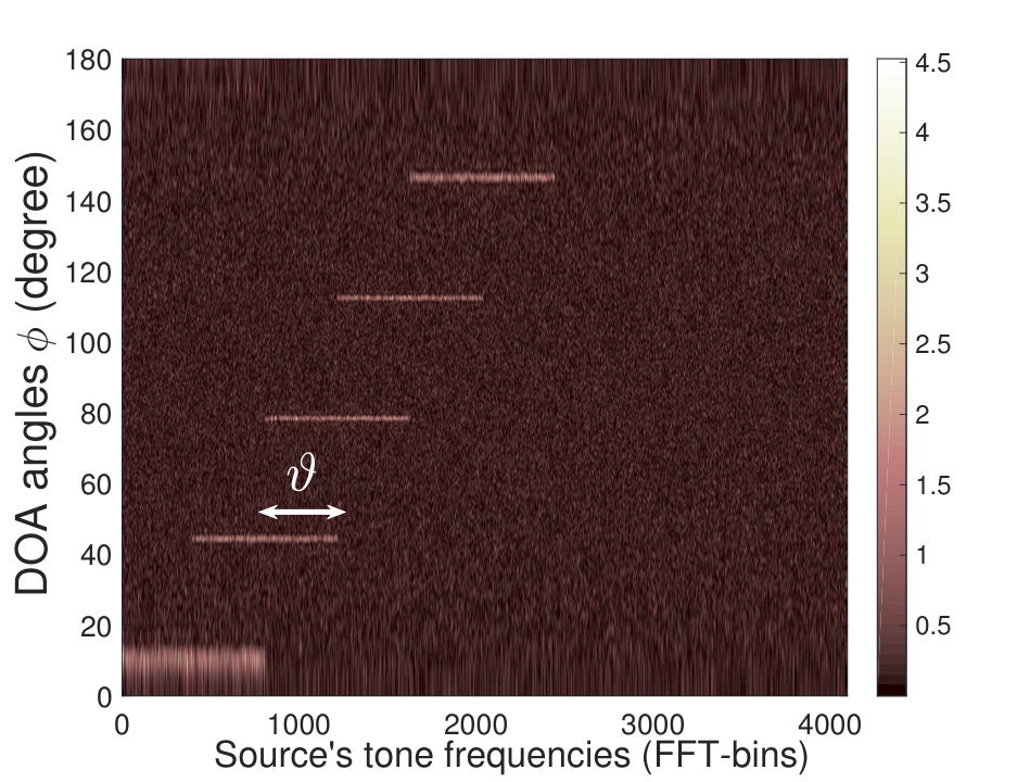
The true amplitudes are ak,m=𝕀m∈[mk,mk+BW]a_{k,m}=\mathbb{I}_{m\in[m_{k},m_{k}+\text{BW}]}, in which mk≜1+(k−1)​⌈(1−ϑ)​BW⌉m_{k}\triangleq 1+(k-1)\left\lceil(1-\vartheta)\text{BW}\right\rceil and the bandwidth of each source is BW=⌊MK⌋\text{BW}=\left\lfloor\frac{M}{K}\right\rfloor, with ⌈⋅⌉\left\lceil\cdot\right\rceil and ⌊⋅⌋\left\lfloor\cdot\right\rfloor denoting the upper- and lower-rounded integer operator, respectively, ∀k∈{1,2,…,K}\forall k\in\{1,2,\ldots,K\}. The overlapping ratio is ϑ∈[0,1]\vartheta\in[0,1], as illustrated in Fig. 4. Note that, the value ϑ=99.9%\vartheta=99.9\% would yield ⌈(1−ϑ)​BW⌉=1\left\lceil(1-\vartheta)\text{BW}\right\rceil=1 FFT-bin, which is the smallest number of non-overlapping tones between two consecutive sources in this setting.

The true DOA angles ϕk=100+(k−1)​Δ​ϕ\phi_{k}=10^{0}+(k-1)\Delta\phi are separated equally over the range [100,1800][10^{0},180^{0}], where DOA’s difference is Δ​ϕ≜⌊1700K⌋\Delta\phi\triangleq\left\lfloor\frac{170^{0}}{K}\right\rfloor, ∀k∈{1,2,…,K}\forall k\in\{1,2,\ldots,K\}. Since DOAs are continuous values and their accuracy also depends on the accuracy of the estimated number of sources, there is no unique way to evaluate the DOA’s estimate error in the DOA’s literature. For this reason, we use a method similar to purity (i.e. successful rate of correct classification) in clustering literature [33]. Let us arrange the true DOA angles ϕ≜[ϕ,1ϕ,2…,ϕK]T\boldsymbol{\phi}\triangleq[\phi{}_{1},\phi{}_{2},\ldots,\phi_{K}]^{T} and their estimates ϕ^≜[ϕ^,1ϕ^,2…,ϕ^K^]T\widehat{\boldsymbol{\phi}}\triangleq[\widehat{\phi}{}_{1},\widehat{\phi}{}_{2},\ldots,\widehat{\phi}_{\widehat{K}}]^{T} in non-decreasing order ϕk≤ϕk+1\phi_{k}\leq\phi_{k+1} and ϕ^k≤ϕ^k+1\widehat{\phi}_{k}\leq\widehat{\phi}_{k+1}, respectively, in which K^\widehat{K} is our estimate of the number KK of sources. The estimate’s error-rate ERR​(ϕ^,ϕ)∈[0,1]\text{ERR}(\widehat{\boldsymbol{\phi}},\boldsymbol{\phi})\in[0,1] is then defined as follows:

ERR​(ϕ^,ϕ)≜𝕀K^=0+𝕀K^>0​1K^​∑j=1K^mink∈{1,2,…,K}⁡|ϕj^−ϕk|1800,\text{ERR}(\widehat{\boldsymbol{\phi}},\boldsymbol{\phi})\triangleq\mathbb{I}_{\widehat{K}=0}+\mathbb{I}_{\widehat{K}>0}\frac{1}{\widehat{K}}\frac{\sum_{j=1}^{\widehat{K}}\min_{k\in\{1,2,\ldots,K\}}|\widehat{\phi_{j}}-\phi_{k}|}{180^{0}}, (41)

and, hence, the error-rate ERR is 100%100\% if K^=0\widehat{K}=0.

For estimate’s error of amplitudes, we use a method similar to Kolmogorov–Smirnov distance for cumulative density function (c.d.f) [34, 35]. Let a^k,m\widehat{a}_{k,m} denote the {k,m}\{k,m\}-element of matrix 𝑨^\widehat{\boldsymbol{A}}, which is our estimate of the true amplitude matrix 𝑨\boldsymbol{A}. Since ak,ma_{k,m} and a^k,m\widehat{a}_{k,m} are associated with true DOAs ϕk\phi_{k} and estimated DOAs ϕ^k\widehat{\phi}_{k}, respectively, let us define the cumulative power spectrums as follows: Fm​(ϕ)≜∫0ϕ∑k=1K‖ak,m‖2​δ​(ϕ−ϕk)​𝑑ϕF_{m}(\phi)\triangleq\int_{0}^{\phi}\sum_{k=1}^{K}||a_{k,m}||^{2}\delta(\phi-\phi_{k})d\phi, and F^m​(ϕ)≜𝕀K^>0​∫0ϕ∑k=1K^‖a^k,m‖2​δ​(ϕ−ϕ^k)​𝑑ϕ\widehat{F}_{m}(\phi)\triangleq\mathbb{I}_{\widehat{K}>0}\int_{0}^{\phi}\sum_{k=1}^{\widehat{K}}||\widehat{a}_{k,m}||^{2}\delta(\phi-\widehat{\phi}_{k})d\phi, in which we set a^k,m=0\widehat{a}_{k,m}=0, ∀k,m\forall k,m, if K^=0\widehat{K}=0. The empirical root mean squared error RMSE​(𝑨^,𝑨)\text{RMSE}(\widehat{\boldsymbol{A}},\boldsymbol{A}) is defined as follows:

RMSE​(𝑨^,𝑨)=1M​∑m=1M∫0180(Fm​(ϕ)−F^m​(ϕ))2​𝑑ϕ.\text{RMSE}(\widehat{\boldsymbol{A}},\boldsymbol{A})=\sqrt{\frac{1}{M}\sum_{m=1}^{M}\int_{0}^{180}(F_{m}(\phi)-\widehat{F}_{m}(\phi))^{2}d\phi}. (42)

We then consider two choices of 𝑨^\widehat{\boldsymbol{A}}: the maximum likelihood (ML) estimate 𝑨0\boldsymbol{A}_{0} in (21) and conditional MAP estimate 𝑨¯\overline{\boldsymbol{A}} in (30).

V-A2 Illustration of overlapping sources via PCA model

Since PCA and MUSIC have the same form of factor analysis in (7), the illustration of their similarity for overlapping multi-tone sources is given in Fig. 4.

When ϑ→0%\vartheta\rightarrow 0\%, there are very few overlapping tones between sources and, hence, there is little correlation between PCA’s components. Note that, the observed data are strongly correlated along each principal vector in this case and, hence, these principal vectors are feasible to detect.

When ϑ→100%\vartheta\rightarrow 100\%, all sources are overlapped with each other and, hence, there is full correlation between PCA’s components. Since the observed data are now uncorrelated for any choice of the principal vectors, the principal vectors become ambiguous and difficult to detect in this case.

We can also see this phenomenon via eigen-decomposition (7, 13) of empirical covariance matrix 𝒀​𝒀∗≈𝑽⁡(𝑨​𝑨∗)​𝑽∗\boldsymbol{Y}\boldsymbol{Y}^{*}\approx\boldsymbol{V}(\boldsymbol{A}\boldsymbol{A}^{*})\boldsymbol{V}^{*} in high SNR scenario. When ϑ→0%\vartheta\rightarrow 0\%, the matrix 𝑨​𝑨∗\boldsymbol{A}\boldsymbol{A}^{*} becomes diagonal and, hence, the kk-th eigenvalue of 𝒀​𝒀∗\boldsymbol{Y}\boldsymbol{Y}^{*} would be a good approximation of the kk-th source’s power ‖𝒂k‖2=𝒂k∗​𝒂k||\boldsymbol{a}_{k}||^{2}=\boldsymbol{a}_{k}^{*}\boldsymbol{a}_{k} in (1, 40). When ϑ→100%,\vartheta\rightarrow 100\%, however, the matrix 𝑨​𝑨∗\boldsymbol{A}\boldsymbol{A}^{*} is close to a constant matrix, whose rank is one. The eigenvalues of 𝒀​𝒀∗\boldsymbol{Y}\boldsymbol{Y}^{*} are not good approximations of source’s powers ‖𝒂k‖2||\boldsymbol{a}_{k}||^{2} anymore and most of the eigenvalues deteriorate to zero in this case, as shown in Fig. 5. Hence, hard-threshold eigen methods do not yield good estimation for the number KK of sources in overlapping case ϑ→100%\vartheta\rightarrow 100\%, even with infinite amount of data. Since AIC for PCA is an eigen-based method, as shown in [16], its performance decreases when the overlapping ratio ϑ\vartheta increases, as shown in Figs. 3-8.

(a) (c) (e)
(b) (d) (f)
Figure 3: Three cases of uncorrelated DOAs: non-overlapping (ϑ=0%\vartheta=0\%), almost overlapping (ϑ=99.9%\vartheta=99.9\%) and completely overlapping (ϑ=100%\vartheta=100\%) for multi-tone sources, with default setting in section V-A1. The legend is the same for all figures. Some curves are almost identical with different values ϑ\vartheta and, hence, indicated by dotted ellipses.
Refer to caption
Figure 4: Illustration of similarity between amplitudes 𝑨\boldsymbol{A} of overlapping multi-tone sources and projected components 𝑨\boldsymbol{A} on principal vectors in PCA. (Left) DTFT power spectrum over FFT-bins, with SNR = 0 dB and ϑ=50%\vartheta=50\% in Fig. 3. (Right) The dots represent the observed data in PCA, with two cases of overlapping ratio ϑ\vartheta.
Figure 5: Eigenvalues (AIC), peaks of power spectrum (DTFT) and peaks of pseudo-spectrum (MUSIC) in descending order, with one Monte Carlo run, SNR=−10\text{SNR}=-10 (dB), ϑ=99.9%\vartheta=99.9\% and the same setting in Fig. 3.

V-A3 MAP estimate versus AIC

The simulations with default setting are given in Fig. 3. Since our MAP estimate K^\widehat{K} (39) is not a hard-threshold eigen method, the performance of DTFT and MUSIC with K^\widehat{K} is almost the same for any overlapping ratios ϑ\vartheta and, hence, is far superior to that of the AIC method in all cases.

In Fig. 3a, it is difficult to estimate KK correctly when SNR<−10\text{SNR}<-10 dB, i.e. maxk⁡σk<σ010=σ03.16\max_{k}\sigma_{k}<\frac{\sigma_{0}}{\sqrt{10}}=\frac{\sigma_{0}}{3.16} in (40). Hence, intuitively, when projected noise’s deviation σ0\sigma_{0} on signal subspace is higher than three empirical deviation of any source’s amplitudes, the noise would completely dominate the signal and it is very hard to extract the signal from noisy data.

Given the estimate of KK in Fig. 3a, the performance of DOA’s estimation via (37) is shown in Fig. 3b. Here we can see that the MAP estimate K^\widehat{K} yields significant improvement for DOA’s estimation accuracy in DTFT and MUSIC algorithms. Although DTFT yields overfitting for the MAP estimate K^\widehat{K} in Fig. 3a, its performance is closer to the case of known KK than the MUSIC and AIC methods. Nonetheless, this is mainly owing to the imperfection of our clustering-based error-rate of DOAs in (41), which becomes lower when there are more estimated sources close to true source’s DOA. Although this error rate is good enough for high SNR, care should be taken for the case of low SNR. Hence, it is safe to say that the credibility of estimated DOAs is very low if SNR<−10\text{SNR}<-10 dB.

Given estimates of DOAs and KK, the RMSE for posterior mean (35) of noise’s deviation σ\sigma is given in Fig. 3c. In non-overlapping case, all methods yield good estimates for σ\sigma. In overlapping cases, our MAP estimate K^\widehat{K} helps DTFT maintain the same performance. In contrast, the eigen-based AIC method yields poor estimates for σ\sigma in overlapping cases, particularly in high SNR. Likewise, since MUSIC is an eigen-based method for the MAP estimation 𝑽^\widehat{\boldsymbol{V}} in (15, 37), it yields worse estimates for σ\sigma in overlapping cases, even with known KK. Nonetheless, our MAP estimate K^\widehat{K} is still much better than AIC in middle SNR with ϑ≤99.9%\vartheta\leq 99.9\%.

From estimate of noise’s deviation in Fig. 3c, the estimate τ¯\overline{\tau} in (36) is then illustrated in Fig. 3d. Since SNR is usually unknown in practice, this estimate τ¯\overline{\tau} is a good indicator of credibility for estimates of KK and DOAs. Indeed, the estimate τ¯\overline{\tau} is consistently around 90%90\%, i.e. σ0≈3​σa\sigma_{0}\approx 3\sigma_{a} in (18), when SNR is around −10-10 (dB). In completely overlapping case, however, the AIC method yields bad estimate for τ¯\overline{\tau} with high SNR.

Given estimates of KK and DOAs in Fig. 3a-b, the RMSE (42) of ML estimate 𝑨0\boldsymbol{A}_{0} is plotted in Fig. 3e. As expected, the eigen-based AIC method is the worst method in overlapping cases, while MAP estimate K^\widehat{K} maintains the good performance for DTFT and MUSIC in all cases of ϑ\vartheta. The DTFT spectrum, when combined with MAP estimate K^\widehat{K}, is better than eigen-based MUSIC in the case ϑ=100%\vartheta=100\% with very high SNR.

When SNR≤−10\text{SNR}\leq-10 dB, the AIC method cannot detect any source in Fig. 3a and, hence, returns zero values for estimated amplitudes in (42). This explains the low RMSE line for amplitude’s estimate of the AIC method in Fig. 3e. Despite being artificial, this zero value of amplitude’s estimate in low SNR is actually a better estimate of amplitudes in terms of RMSE. Indeed, as shown in Fig. 3f, the MAP estimate 𝑨¯=(1−τ¯)​𝑨0\overline{\boldsymbol{A}}=(1-\overline{\tau})\boldsymbol{A}_{0} in (30) yields lower RMSE than ML estimate 𝑨0\boldsymbol{A}_{0} since 𝑨¯\overline{\boldsymbol{A}} can automatically switch to zero value if SNR is too low, which is indicated by the estimate τ¯\overline{\tau} in Fig. 3d.

For illustration, the critical case of SNR=−10\text{SNR}=-10 dB in Fig. 3 is shown in Fig. 5. We can see that the peaks in DTFT and MUSIC spectrums linearly decrease with KK and, hence, there is no clear difference between noise’s peaks and signal’s peaks around K=5K=5 in this low SNR regime. It is then difficult to extract the correct number K=5K=5 of sources from these spectrum’s peaks. In contrast, the MAP criterion (39) reaches the peak at K^=5\widehat{K}=5, since it can return the maximum difference among all possible binomial combinations of signal and noise subspaces via (33-34). The MAP estimate K^\widehat{K} is therefore the best estimate in this case.

Figure 6: Simulations for the case of moderately correlated DOAs (D=15D=15 sensors), with the same default setting in Fig. 3. The first row is DTFT and MUSIC spectrums for the case SNR=−10\text{SNR}=-10 (dB) and non-overlapping (ϑ=0%\vartheta=0\%), with the same convention in Fig. 5. The legend is the same for all figures in other rows.
Figure 7: Simulations for the case of highly correlated DOAs (Δ​ϕ=40\Delta\phi=4^{0}), with the same default setting in Fig. 3. The first row is DTFT and MUSIC spectrums for the case SNR=−10\text{SNR}=-10 (dB) and non-overlapping (ϑ=0%\vartheta=0\%), with the same convention in Fig. 5. The legend is the same for all figures in other rows.
Figure 8: Simulations for the case of decayed amplitudes, with the same legend and default setting in Fig. 3. The first row is DTFT and MUSIC spectrums for the case SNR=0\text{SNR}=0 (dB), non-overlapping (ϑ=0%\vartheta=0\%) and decayed ratio ψ=80%\psi=80\%, with the same convention in Fig. 5. The legend is the same for all figures in other rows.

V-B Correlated multi-tone sources

As explained above, both DTFT spectrum and MUSIC algorithm can yield good estimates for all cases of uncorrelated DOAs, when combined with MAP estimate K^\widehat{K}. The eigen-based AIC method, however, yields the worst estimates for overlapping multi-tone sources.

In this subsection, let us consider the case of correlated DOAs. Since the uncorrelated condition (6, 7) for PCA and MUSIC models is violated in this case, their estimates 𝑽^\widehat{\boldsymbol{V}} and K^\widehat{K} in (37, 39) are not exact MAP estimates anymore, but merely approximations. Hence, the optimal performance of estimates 𝑽^\widehat{\boldsymbol{V}} and K^\widehat{K} is not guaranteed in this case.

From default setting, the number of sensors is reduced from D=100D=100 to D=15D=15 in Fig. 6. In this case of moderate correlation, the performance is still similar to the uncorrelated case of default setting. The estimate of KK in DTFT, however, switches from overfitting to underfitting in Fig. 6. The performance of non eigen-based DTFT is similar to that of eigen-based MUSIC algorithm in non-overlapping case ϑ=0%\vartheta=0\%, but becomes better in nearly overlapping case ϑ=99.9%\vartheta=99.9\%. The approximated MAP estimate K^\widehat{K} (39) in this case is still much better than the AIC method, although their performance in this correlated case is worse than default setting. The estimate τ¯\overline{\tau} is still a useful indicator for detecting the limit SNR=−10\text{SNR}=-10 (dB), although it is not suitable for the AIC method in nearly overlapping case ϑ=99.9%\vartheta=99.9\%.

In Fig. 7, the DOA’s difference is reduced gradually from Δ​ϕ=340\Delta\phi=34^{0} in default setting to Δ​ϕ=40\Delta\phi=4^{0}. For Δ​ϕ≤40\Delta\phi\leq 4^{0}, we found that the approximated MAP K^\widehat{K} in the DTFT method began yielding inaccurate estimates in middle SNR. Intuitively, when DOA’s difference Δ​ϕ\Delta\phi is too small, the superposition of peaks of power leakage in Fig. 2 will become comparable with the spectrum’s peaks of sources, as illustrated in first row of Fig. 7. Hence, it is harder for the DTFT method to extract the correct peaks of sources and to return the correct MAP estimate K^\widehat{K}. Also, since this setting of low Δ​ϕ\Delta\phi yields higher correlation than setting of low D=15D=15, the MAP estimate K^\widehat{K} in MUSIC is slightly worse than the case of D=15D=15 in Fig. 6. Our estimate K^\widehat{K} is, nonetheless, still much better than the AIC method overall. The estimate τ¯\overline{\tau} is still a useful indicator for detecting the limit SNR=−10\text{SNR}=-10 (dB) in this case.

V-C Decayed multi-tone sources

In this subsection, we will study the case of uncorrelated DOAs with different amplitudes. From default setting, we now set ak,m=(1−ψ​k−1K)​𝕀m∈[mk,mk+BW]a_{k,m}=(1-\psi\frac{k-1}{K})\mathbb{I}_{m\in[m_{k},m_{k}+\text{BW}]}, ∀k∈{1,2,…,K}\forall k\in\{1,2,\ldots,K\}, in which the decayed ratio is ψ∈[0,1]\psi\in[0,1]. The simulations with different values ψ\psi are given in Fig. 8.

Since there is a power leakage, even for uncorrelated DOAs, as illustrated in Fig. 2, the strongly decayed amplitudes will be confused with this power leakage. Indeed, there are six DTFT peaks instead of the ground-truth K=5K=5 peaks in first row of Fig. 8. Hence, for middle SNR regime, the estimate’s accuracy of this case is worse than that of the default setting in Fig. 3. Nonetheless, the estimate’s accuracy of amplitudes and τ¯\overline{\tau} for all methods in this case is not much different from default setting, for all cases of SNR.

In the case of non-overlapping ϑ=0%\vartheta=0\% in Fig. 8, the MAP estimate K^\widehat{K} is superior to that by the AIC method in moderately decayed setting ψ=50%\psi=50\%, although it is worse than the AIC method in middle SNR regime of strongly decayed setting ψ=90%\psi=90\%. The reason for this is likely owing to our amplitude’s prior in (18, 24), which takes into account the average of all amplitude’s variances. The decision of our MAP estimate K^\widehat{K} is, hence, influenced by the average value of all decayed amplitudes, instead of each decayed amplitude separately. This decayed setting suggests that we may have to consider individual decayed amplitudes for the MAP estimate K^\widehat{K} in future works.

In the case of almost overlapping ϑ=99.9%\vartheta=99.9\% in Fig. 8, nonetheless, the MAP estimate K^\widehat{K} is still much superior to AIC method, since our MAP criterion (38, 39) is not an eigen-based method, as explained in default setting above.

VI Conclusion

In this paper, we have derived a closed-form solution for MAP estimate of the number KK of sources in PCA, MUSIC and DTFT spectrum methods. For this purpose, we have also derived two novel probability distributions, namely double gamma and double inverse-gamma distributions. Owing to these distributions, we recognized that the posterior probability distribution of KK takes into account all possible binomial combinations of signal and noise subspaces in noisy data space. The MAP estimate of KK then corresponds to the dimension of signal subspace with highest probability of domination of signal-plus-noise’s variance over noise’s variance.

In simulations of linear sensor array, we also recognized that, for accurate estimation, the SNR of maximum signal’s power should be higher than −10-10dB, which means the estimated noise-to-signal percentage τ¯\overline{\tau} should be less than 90%90\% (i.e. the projected noise’s deviation on signal space should be less than three deviation of source’s amplitudes).

For overlapping multi-tone sources, our MAP estimate method was shown to be far superior to eigen-based methods like Akaike information criterion (AIC) for PCA. Our MAP estimate method is, however, only based on averaged value of amplitude’s variances and uncorrelated principal/steering vectors. The MAP estimates for individual amplitudes and correlated principal vectors are, hence, interesting cases for future works.

Appendix A Negative binomial and double gamma distributions

In this Appendix, let us derive two novel distributions, namely double gamma and double inverse-gamma distributions, which were used for estimating the signal’s and noise’s variance in section IV-C3. For this purpose, let us firstly show the relationship between negative binomial distribution and order statistics of two independent gamma distributions, as follows:

Theorem 1.

(Negative binomial distribution) Let X∼𝒢X​(n,s)X\sim\mathcal{G}_{X}(n,s) and Y∼𝒢Y​(m,t)Y\sim\mathcal{G}_{Y}(m,t) be random variables (r.v.) of two independent gamma distributions, with positive integers nn, mm being the degree of freedom. The probability of the event X≤YX\leq Y is:

Pr⁡[𝕀X≤Y]\displaystyle\Pr[\mathbb{I}_{X\leq Y}] =Ip​(n,m)=1−I1−p​(m,n),with​p≜ss+t,\displaystyle=I_{p}(n,m)=1-I_{1-p}(m,n),\ \text{with}\ p\triangleq\frac{s}{s+t}, (43)

where 𝕀X≤Y\mathbb{I}_{X\leq Y} is the boolean indicator function, Ip​(n,m)=∫0ptn−1​(1−t)m−1​𝑑tB⁡(n,m)I_{p}(n,m)=\frac{\int_{0}^{p}t^{n-1}(1-t)^{m-1}dt}{B(n,m)} is the regularized incomplete beta function and:

Ip​(n,m)\displaystyle I_{p}(n,m) =1−∑k=0n−1(m+k−1k)​(1−p)m​pk⏟𝒩​ℬk​(m,p)\displaystyle=1-\underset{\mathcal{NB}_{k}(m,p)}{\sum_{k=0}^{n-1}\underbrace{\left(\begin{array}[]{c}m+k-1\\ k\end{array}\right)(1-p)^{m}p^{k}}}
=1−I1−p​(m,n)=∑k=0m−1𝒩​ℬk​(n,1−p),\displaystyle=1-I_{1-p}(m,n)=\sum_{k=0}^{m-1}\mathcal{NB}_{k}(n,1-p),

with (nk)≜n!(n−k)!​k!\left(\begin{array}[]{c}n\\ k\end{array}\right)\triangleq\frac{n!}{(n-k)!k!} denoting binomial coefficient.

Note that, Ip​(n,m)I_{p}(n,m) is actually the cumulative mass function (c.m.f) of a negative binomial distribution 𝒩​ℬk​(n,1−p)\mathcal{NB}_{k}(n,1-p), ∀k∈{0,1​…,∞}\forall k\in\{0,1\ldots,\infty\}. Likewise, the reverse form I1−p​(m,n)=1−Ip​(n,m)I_{1-p}(m,n)=1-I_{p}(n,m) is the c.m.f of 𝒩​ℬk​(m,p)\mathcal{NB}_{k}(m,p) in (1). Hence, we also have Ip​(n,m)=∑k=n+∞𝒩​ℬk​(m,p)I_{p}(n,m)=\sum_{k=n}^{+\infty}\mathcal{NB}_{k}(m,p), i.e. the reverse c.m.f. of 𝒩​ℬk​(m,p)\mathcal{NB}_{k}(m,p).

Let us prove Theorem 1 together with Corollary 2 below.

Corollary 2.

(Double gamma distributions) In Theorem 1, the conditional probability distribution function (p.d.f) of XX given YY is the right-truncated gamma distribution, while the marginal p.d.f of XX and YY are called the lower- and upper-double gamma distributions, respectively, as follows:

f⁡(X|Y,𝕀X≤Y)\displaystyle f(X|Y,\mathbb{I}_{X\leq Y}) =𝒢X≤Y​(n,s)≜𝒢X​(n,s)γ⁡(n,s​Y)Γ⁡(n),\displaystyle=\mathcal{G}_{X\leq Y}(n,s)\triangleq\frac{\mathcal{G}_{X}(n,s)}{\frac{\gamma(n,sY)}{\Gamma(n)}}, (46)
f⁡(X|𝕀X≤Y)\displaystyle f(X|\mathbb{I}_{X\leq Y}) =𝒢​𝒢X​(n,m,s,t)≜Γ⁡(m,t​X)Γ⁡(m)​𝒢X​(n,s)Ip​(n,m),\displaystyle=\mathcal{G}\mathcal{G}_{X}(n,m,s,t)\triangleq\frac{\Gamma\left(m,tX\right)}{\Gamma(m)}\frac{\mathcal{G}_{X}(n,s)}{I_{p}(n,m)},
f⁡(Y|𝕀X≤Y)\displaystyle f(Y|\mathbb{I}_{X\leq Y}) =𝒢​𝒢​𝒰Y​(n,m,s,t)≜γ⁡(n,s​Y)Γ⁡(n)​𝒢Y​(m,t)Ip​(n,m),\displaystyle=\mathcal{G}\mathcal{G}\mathcal{U}_{Y}(n,m,s,t)\triangleq\frac{\gamma(n,sY)}{\Gamma(n)}\frac{\mathcal{G}_{Y}(m,t)}{I_{p}(n,m)},

where γ⁡(n,x)=Γ⁡(n)−Γ⁡(n,x)\gamma(n,x)=\Gamma(n)-\Gamma(n,x) and Γ⁡(n,x)\Gamma(n,x) denote the lower and upper incomplete gamma functions, respectively, with Γ⁡(n)=(n−1)!\Gamma(n)=(n-1)! denoting the gamma function. Then, their kk-th moments are:

Xk¯\displaystyle\overline{X^{k}} =𝔼f⁡(X|𝕀X≤Y)​Xk=Γ⁡(n+k)sk​Γ​(n)​Ip​(n+k,m)Ip​(n,m),\displaystyle=\mathbb{E}_{f(X|\mathbb{I}_{X\leq Y})}X^{k}=\frac{\Gamma(n+k)}{s^{k}\Gamma(n)}\frac{I_{p}(n+k,m)}{I_{p}(n,m)},
Yk¯\displaystyle\overline{Y^{k}} =𝔼f⁡(Y|𝕀X≤Y)​Yk=Γ⁡(m+k)tk​Γ​(m)​Ip​(n,m+k)Ip​(n,m).\displaystyle=\mathbb{E}_{f(Y|\mathbb{I}_{X\leq Y})}Y^{k}=\frac{\Gamma(m+k)}{t^{k}\Gamma(m)}\frac{I_{p}(n,m+k)}{I_{p}(n,m)}. (47)
Proof:

Firstly, the conditional probability mass function (p.m.f) of 𝕀X≤Y\mathbb{I}_{X\leq Y} is Pr[𝕀X≤Y|X,Y]=𝕀X≤Y\text{Pr}[\mathbb{I}_{X\leq Y}|X,Y]=\mathbb{I}_{X\leq Y}. The joint distribution is then:

f⁡(X,Y,𝕀X≤Y)\displaystyle f(X,Y,\mathbb{I}_{X\leq Y}) =Pr[𝕀X≤Y|X,Y]f(X)f(Y)\displaystyle=\text{Pr}[\mathbb{I}_{X\leq Y}|X,Y]f(X)f(Y)
=f⁡(X|Y,𝕀X≤Y)​Pr​[𝕀X≤Y|Y]​f​(Y)\displaystyle=f(X|Y,\mathbb{I}_{X\leq Y})\text{Pr}[\mathbb{I}_{X\leq Y}|Y]f(Y)
=f⁡(X|Y,𝕀X≤Y)​f​(Y|𝕀X≤Y)​Pr​[𝕀X≤Y],\displaystyle=f(X|Y,\mathbb{I}_{X\leq Y})f(Y|\mathbb{I}_{X\leq Y})\text{Pr}[\mathbb{I}_{X\leq Y}],

in which, by Bayes’ rule, the posterior f⁡(X|Y,𝕀X≤Y)=Pr[𝕀X≤Y|X,Y]f(X)Pr​[𝕀X≤Y|Y]f(X|Y,\mathbb{I}_{X\leq Y})=\frac{\text{Pr}[\mathbb{I}_{X\leq Y}|X,Y]f(X)}{\text{Pr}[\mathbb{I}_{X\leq Y}|Y]} is right-truncated inverse-gamma distribution in (46), since Pr[𝕀X≤Y|Y]=∫0YPr[𝕀X≤Y|X,Y]f(X)dX=𝕀X≤Y∫0X𝒢X(s,t)dY=𝕀X≤Yγ⁡(s,t​Y)Γ⁡(s)\text{Pr}[\mathbb{I}_{X\leq Y}|Y]=\int_{0}^{Y}\text{Pr}[\mathbb{I}_{X\leq Y}|X,Y]f(X)dX=\mathbb{I}_{X\leq Y}\int_{0}^{X}\mathcal{G}_{X}(s,t)dY=\mathbb{I}_{X\leq Y}\frac{\gamma(s,tY)}{\Gamma(s)}. Likewise, the Bayes’ rule yields f⁡(Y|𝕀X≤Y)=Pr​[𝕀X≤Y|Y]​f​(Y)Pr​[𝕀X≤Y]f(Y|\mathbb{I}_{X\leq Y})=\frac{\text{Pr}[\mathbb{I}_{X\leq Y}|Y]f(Y)}{\text{Pr}[\mathbb{I}_{X\leq Y}]} in (46), as follows:

Pr⁡[𝕀X≤Y]\displaystyle\Pr[\mathbb{I}_{X\leq Y}] =∫0∞Pr​[𝕀X≤Y|Y]​f​(Y)​𝑑Y\displaystyle=\int_{0}^{\infty}\text{Pr}[\mathbb{I}_{X\leq Y}|Y]f(Y)dY (48)
=𝕀X≤Y​∫0∞γ⁡(n,s​Y)Γ⁡(n)​𝒢Y​(m,t)​𝑑Y,\displaystyle=\mathbb{I}_{X\leq Y}\int_{0}^{\infty}\frac{\gamma(n,sY)}{\Gamma(n)}\mathcal{G}_{Y}\left(m,t\right)dY,

Solving (48) via series form γ⁡(n,x)Γ⁡(n)=1−∑k=0n−1xk​e−xk!\frac{\gamma(n,x)}{\Gamma(n)}=1-\sum_{k=0}^{n-1}\frac{x^{k}e^{-x}}{k!} and expectation of gamma distribution 𝒢x​(α,β)=βαΓ⁡(α)​xα−1​e−β​x\mathcal{G}_{x}\left(\alpha,\beta\right)=\frac{\beta^{\alpha}}{\Gamma(\alpha)}x^{\alpha-1}e^{-\beta x}, we obtain:

∫0∞γ⁡(n,s​Y)Γ⁡(n)​𝒢Y​(m,t)​𝑑Y\displaystyle\int_{0}^{\infty}\frac{\gamma(n,sY)}{\Gamma(n)}\mathcal{G}_{Y}\left(m,t\right)dY =1−∑k=0n−1Γ⁡(m+k)Γ⁡(m)​k!​tm​sk(t+s)m+k\displaystyle=1-\sum_{k=0}^{n-1}\frac{\Gamma(m+k)}{\Gamma(m)k!}\frac{t^{m}s^{k}}{(t+s)^{m+k}}
=Iss+t​(n,m),\displaystyle=I_{\frac{s}{s+t}}(n,m),

which yields (43). Similarly, we can compute f⁡(X|𝕀X≤Y)=∫X∞f⁡(X|Y,𝕀X≤Y)​f​(Y|𝕀X≤Y)​𝑑Yf(X|\mathbb{I}_{X\leq Y})=\int_{X}^{\infty}f(X|Y,\mathbb{I}_{X\leq Y})f(Y|\mathbb{I}_{X\leq Y})dY in (46). Also, we have: Xk​𝒢X​(n,s)=Γ⁡(n+k)sk​Γ​(n)​𝒢X​(n+k,t)X^{k}\mathcal{G}_{X}(n,s)=\frac{\Gamma(n+k)}{s^{k}\Gamma(n)}\mathcal{G}_{X}(n+k,t), hence the moments (47). ∎By simply changing the gamma distribution to inverse-gamma distribution, we can extend the above results to inverse-gamma distributions feasibly, as follows:

Corollary 3.

(Double inverse-gamma distributions) Similar to Theorem 1 and Corollary 2, let X∼i​𝒢X​(n,s)X\sim i\mathcal{G}_{X}(n,s) and Y∼𝒢Y​(m,t)Y\sim\mathcal{G}_{Y}(m,t) be r.v. of independent inverse-gamma distributions, with positive integers nn, mm. If X≥Y,X\geq Y, the conditional p.d.f of XX given YY is the left-truncated inverse-gamma distribution, while the marginal p.d.f of XX and YY are called the upper- and lower-double inverse-gamma distributions, respectively, as follows:

f⁡(X|Y,𝕀X≥Y)\displaystyle f(X|Y,\mathbb{I}_{X\geq Y}) =i​𝒢X≥Y​(n,s)≜i​𝒢X​(n,s)γ⁡(n,sY)Γ⁡(n),\displaystyle=i\mathcal{G}_{X\geq Y}(n,s)\triangleq\frac{i\mathcal{G}_{X}(n,s)}{\frac{\gamma(n,\frac{s}{Y})}{\Gamma(n)}}, (49)
f⁡(X|𝕀X≥Y)\displaystyle f(X|\mathbb{I}_{X\geq Y}) =i​𝒢​𝒢​𝒰X​(n,m,s,t)≜Γ⁡(m,tX)Γ⁡(m)​i​𝒢X​(n,s)Ip​(n,m),\displaystyle=i\mathcal{G}\mathcal{G}\mathcal{U}_{X}(n,m,s,t)\triangleq\frac{\Gamma\left(m,\frac{t}{X}\right)}{\Gamma(m)}\frac{i\mathcal{G}_{X}(n,s)}{I_{p}(n,m)},
f⁡(Y|𝕀X≥Y)\displaystyle f(Y|\mathbb{I}_{X\geq Y}) =i​𝒢​𝒢Y​(n,m,s,t)≜γ⁡(n,sY)Γ⁡(n)​i​𝒢Y​(m,t)Ip​(n,m),\displaystyle=i\mathcal{G}\mathcal{G}_{Y}(n,m,s,t)\triangleq\frac{\gamma(n,\frac{s}{Y})}{\Gamma(n)}\frac{i\mathcal{G}_{Y}(m,t)}{I_{p}(n,m)},

with Pr⁡[𝕀X≥Y]=Ip​(n,m),\Pr[\mathbb{I}_{X\geq Y}]=I_{p}(n,m), p≜ss+tp\triangleq\frac{s}{s+t} and Ip​(n,m)I_{p}(n,m) given in (43, 1). Then, similar to (47), the moments for (49) are:

Xk¯\displaystyle\overline{X^{k}} =𝔼f⁡(X|𝕀X≥Y)​Xk=Γ⁡(n−k)s−k​Γ​(n)​Ip​(n−k,m)Ip​(n,m),\displaystyle=\mathbb{E}_{f(X|\mathbb{I}_{X\geq Y})}X^{k}=\frac{\Gamma(n-k)}{s^{-k}\Gamma(n)}\frac{I_{p}(n-k,m)}{I_{p}(n,m)},
Yk¯\displaystyle\overline{Y^{k}} =𝔼f⁡(Y|𝕀X≥Y)​Yk=Γ⁡(m−k)t−k​Γ​(m)​Ip​(n,m−k)Ip​(n,m).\displaystyle=\mathbb{E}_{f(Y|\mathbb{I}_{X\geq Y})}Y^{k}=\frac{\Gamma(m-k)}{t^{-k}\Gamma(m)}\frac{I_{p}(n,m-k)}{I_{p}(n,m)}. (50)

Appendix B Bayesian minimum-risk estimation

Let us briefly review the importance of posterior distributions in practice, via minimum-risk property of Bayesian estimation method. Without loss of generalization, let us assume that the unknown parameter θ\theta in our model is continuous. In practice, the aim is often to return estimated value θ^≜θ^​(𝑿)\hat{\theta}\triangleq\hat{\theta}(\boldsymbol{X}), as a function of noisy data 𝑿\boldsymbol{X}, with minimum mean squared error MSE​(θ^,θ)≜𝔼f⁡(𝑿,θ)​‖θ^​(𝑿)−θ‖22\text{MSE}(\hat{\theta},\theta)\triangleq\mathbb{E}_{f(\boldsymbol{X},\theta)}||\hat{\theta}(\boldsymbol{X})-\theta||_{2}^{2}, where ||⋅||2||\cdot||_{2} is ℒ2\mathcal{L}_{2}-normed operator. Then, by basic chain rule of probability f⁡(𝑿,θ)=f⁡(θ|𝑿)​f​(𝑿)f(\boldsymbol{X},\theta)=f(\theta|\boldsymbol{X})f(\boldsymbol{X}), we have [35, 36]:

θ^\displaystyle\hat{\theta} ≜arg​minθ~⁡MSE​(θ~,θ)\displaystyle\triangleq\operatornamewithlimits{arg\,min}_{\tilde{\theta}}\text{MSE}(\tilde{\theta},\theta)
=arg​minθ~⁡𝔼f⁡(θ|𝑿)​‖θ~​(𝑿)−θ‖22\displaystyle=\operatornamewithlimits{arg\,min}_{\tilde{\theta}}\mathbb{E}_{f(\theta|\boldsymbol{X})}||\tilde{\theta}(\boldsymbol{X})-\theta||_{2}^{2} (51)
=𝔼f⁡(θ|𝑿)​(θ),\displaystyle=\mathbb{E}_{f(\theta|\boldsymbol{X})}(\theta),

which shows that the posterior mean θ^=𝔼f⁡(θ|𝑿)​(θ)\hat{\theta}=\mathbb{E}_{f(\theta|\boldsymbol{X})}(\theta) is the minimum MSE (MMSE) estimate. In general, we may replace the ℒ2\mathcal{L}_{2}-norm in (51) by other normed functions. For example, it is well-known that the best estimators for averaged ℒ1\mathcal{L}_{1} and ℒ∞\mathcal{L}_{\infty}-normed error are posterior median and mode of f⁡(θ|𝑿)f(\theta|\boldsymbol{X}), respectively [35, 36].

References

  • [1] Z. Yang and L. Xie, “Enhancing sparsity and resolution via reweighted atomic norm minimization,” IEEE Transactions on Signal Processing, vol. 64, no. 4, pp. 995–1006, Feb. 2016.
  • [2] B. N. Bhaskar, G. Tang, and B. Recht, “Atomic norm denoising with applications to line spectral estimation,” IEEE Transactions on Signal Processing, vol. 61, no. 23, pp. 5987–5999, Dec. 2013.
  • [3] M.-A. Badiu, T. L. Hansen, and B. H. Fleury, “Variational Bayesian inference of line spectra,” IEEE Transactions on Signal Processing, vol. 65, no. 9, pp. 2247–2261, May 2017.
  • [4] Z. Zhang, S. Wang, D. Liu, and M. I. Jordan, “EP-GIG priors and applications in Bayesian sparse learning,” J. Mach. Learn. Res., vol. 13, pp. 2031–2061, Jun. 2012.
  • [5] C. F. Mecklenbrauker, P. Gerstoft, A. Panahi, and M. Viberg, “Sequential Bayesian sparse signal reconstruction using array data,” IEEE Transactions on Signal Processing, vol. 61, no. 24, pp. 6344–6354, Dec. 2013.
  • [6] M. Hawes, L. Mihaylova, F. Septier, and S. Godsill, “Bayesian compressive sensing approaches for direction of arrival estimation with mutual coupling effects,” IEEE Transactions on Antennas and Propagation, vol. 65, no. 3, pp. 1357–1368, Mar. 2017.
  • [7] J. Dai, X. Bao, W. Xu, and C. Chang, “Root sparse Bayesian learning for off-grid DOA estimation,” IEEE Signal Processing Letters, vol. 24, no. 1, pp. 46–50, Jan. 2017.
  • [8] G. Tang, B. N. Bhaskar, and B. Recht, “Near minimax line spectral estimation,” IEEE Transactions on Information Theory, vol. 61, no. 1, pp. 499–512, Jan. 2015.
  • [9] J. G. Proakis and D. K. Manolakis, Digital Signal Processing, 4th ed. Pearson, 2006.
  • [10] A. E. Gonnouni, M. Martinez-Ramon, J. L. Rojo-Alvarez, G. Camps-Valls, A. R. Figueiras-Vidal, and C. G. Christodoulou, “A support vector machine MUSIC algorithm,” IEEE Transactions on Antennas and Propagation, vol. 60, no. 10, pp. 4901–4910, Oct. 2012.
  • [11] A. L. Kintz and I. J. Gupta, “A modified MUSIC algorithm for direction of arrival estimation in the presence of antenna array manifold mismatch,” IEEE Transactions on Antennas and Propagation, vol. 64, no. 11, pp. 4836–4847, Nov. 2016.
  • [12] T. Lavate, V. Kokate, and A. Sapkal, “Performance analysis of MUSIC and ESPRIT DOA estimation algorithms for adaptive array smart antenna in mobile communication,” Second International Conference on Computer and Network Technology (ICCNT), 2010.
  • [13] O. A. Oumar, M. F. Siyau, and T. P. Sattar, “Comparison between MUSIC and ESPRIT direction of arrival estimation algorithms for wireless communication systems,” International Conference on Future Generation Communication Technology (FGCT), 2012.
  • [14] K. Han and A. Nehorai, “Improved source number detection and direction estimation with nested arrays and ULAs using jackknifing,” IEEE Transactions on Signal Processing, vol. 61, no. 23, pp. 6118–6128, Dec. 2013.
  • [15] E. Fishler, M. Grosmann, and H. Messer, “Detection of signals by information theoretic criteria: general asymptotic performance analysis,” IEEE Transactions on Signal Processing, vol. 50, no. 5, pp. 1027–1036, May 2002.
  • [16] H. L. V. Trees, Optimum Array Processing: Part IV of Detection, Estimation, and Modulation Theory. Wiley-Interscience, 2002.
  • [17] H. Akaike, “A new look at the statistical model identification,” IEEE Trans. Autom. Control, vol. 19, pp. 716–723, Dec. 1974.
  • [18] M. Gavish and D. L. Donoho, “The optimal hard threshold for singular values is 4/sqrt(3),” IEEE Transactions on Information Theory, vol. 60, no. 8, pp. 5040–5053, 2014.
  • [19] P. Karl, “On lines and planes of closest fit to systems of points in space,” The London, Edinburgh and Dublin Philosophical Magazine and Journal of Science, vol. 2, no. 11, pp. 559–572, 1901.
  • [20] H. Hotelling, “Analysis of a complex of statistical variables into principal components,” Journal of Educational Psychology, vol. 24, no. 6, pp. 417–441, 1933.
  • [21] I. T. Jolliffe and J. Cadima, “Principal component analysis - a review and recent developments,” Philosophical Transactions of the Royal Society of London A - Mathematical, Physical and Engineering Sciences, vol. 374, pp. 1–16, 2016.
  • [22] M. E. Tipping and C. M. Bishop, “Probabilistic principal component analysis,” Journal of the Royal Statistical Society, series B (Statistical Methodology), vol. 61, no. 3, pp. 611–622, 1999.
  • [23] V. Smidl and A. Quinn, “On Bayesian principal component analysis,” Computational Statistics & Data Analysis, vol. 51, pp. 4101–4123, Feb. 2007.
  • [24] O. Besson, N. Dobigeon, and J.-Y. Tourneret, “Minimum mean square distance estimation of a subspace,” IEEE Transactions on Signal Processing, vol. 59, no. 12, pp. 5709–5720, Dec. 2011.
  • [25] P.-A. Mattei, “Model selection for sparse high-dimensional learning,” Ph.D. dissertation, Université Paris Descartes, 2017.
  • [26] C. Elvira, P. Chainais, and N. Dobigeon, “Bayesian nonparametric subspace estimation,” IEEE International Conference on Acoustics, Speech and Signal Processing (ICASSP), pp. 2247–2251, Jun. 2017.
  • [27] C. Elvira, “Modèles Bayésiens pour l’identification de représentations antiparcimonieuses et l’analyse en composantes principales Bayésienne non paramétrique,” Ph.D. dissertation, Ecole Centrale de Lille, 2017.
  • [28] T. P. Minka, “Automatic choice of dimensionality for PCA,” Neural Information Processing Systems (NIPS) Conference, vol. 13, pp. 598–604, Jan. 2000.
  • [29] V. H. Tran, W. Wang, Y. Luo, and J. Chambers, “Bayesian inference for multi-line spectra in linear sensor array,” IEEE International Conference on Acoustics, Speech and Signal Processing (ICASSP), Apr. 2018.
  • [30] H. Araki and S. Yamagami, “An inequality for Hilbert-Schmidt norm,” Communications in Mathematical Physics, vol. 81, no. 1, pp. 89–96, Sep. 1981.
  • [31] H. H. Andersen, M. Hojbjerre, D. Sorensen, and P. S. Eriksen, Linear and Graphical Models for the Multivariate Complex Normal Distribution. Springer Science & Business Media, 1995.
  • [32] O. Henkel, “Sphere-packing bounds in the Grassmann and Stiefel manifolds,” IEEE Transactions on Information Theory, vol. 51, no. 10, pp. 3445–3456, Oct. 2005.
  • [33] P.-N. Tan, M. Steinbach, and V. Kumar, Introduction to Data Mining. Addison-Wesley, Boston, 2006.
  • [34] S. T. Rachev, Probability Metrics and Stability of Stochastic Models. John Wiley & Sons, 1991.
  • [35] V. H. Tran, “Variational Bayes inference in digital receivers,” Ph.D. dissertation, Trinity College Dublin, 2014.
  • [36] J. M. Bernardo and A. F. M. Smith, Bayesian Theory. John Wiley & Sons Canada, 2006.