Echo trains in pulsed electron spin resonance of a strongly coupled spin ensemble
Abstract
We report on a novel dynamical phenomenon in electron spin resonance experiments of phosphorus donors. When strongly coupling the paramagnetic ensemble to a superconducting lumped element resonator, the coherent exchange between these two subsystems leads to a train of periodic, self-stimulated echos after a conventional Hahn echo pulse sequence. The presence of these multi-echo signatures is explained using a simple model based on spins rotating on the Bloch sphere, backed up by numerical calculations using the inhomogeneous Tavis-Cummings Hamiltonian.
pacs
03.67.Lx, 42.50.Ct, 42.50.Pq, 76.30.-vPulsed electron spin resonance (ESR) is an essential spectroscopy technique used in many fields of science, e.g., for the study of the structure and dynamics of molecular systems [1, 2], for material science [3] as well as for quantum sensing and information applications [4, 5, 6]. To implement this technique, a vast repertoire of sophisticated pulse sequences exists [7], each of them optimized to investigate particular spin properties. Nevertheless, the majority of the sequences is based on a Hahn echo [8] as schematically shown in Fig. 1 (a).
A newly emerging area for ESR experiments is the processing of quantum information. Using superconducting microwave resonators, the so-called “strong coupling regime” has recently been demonstrated [9, 10, 11, 12, 13, 14]. Here, the coherent exchange of information between the microwave resonator and the spin ensemble exceeds the individual decay rates of the two subsystems, which is a requirement for applications involving the storage and conversion of quantum information [15, 9, 16, 17]. Apart from its importance for quantum technology, a strong coupling rate also enhances the sensitivity in ESR applications [18, 19] going beyond classical ESR models [7, 20]. First seminal experiments in the presence of strong spin-photon coupling revealed a plethora of new physical effects [13, 21, 22, 23]. A fascinating question that remains unresolved, however, is what happens when the Hahn echo is transferred to the context of a strongly coupled spin ensemble.
To explore this question experimentally, we work with a superconducting microwave resonator strongly coupled to a paramagnetic spin ensemble. Specifically, we compare pulsed ESR measurements of a strongly coupled spin ensemble based on isolated phosphorus donors in a 28Si host matrix with a weakly coupled ensemble of P2 dimers also present in the sample. In the weak coupling case, as in a conventional ESR experiment, we observe a single Hahn echo in terms of a photon pulse that is emitted into the resonator at when the spins refocus, where is the inter-pulse delay. In stark contrast, when applying the same Hahn echo sequence in the strong coupling regime, we observe a periodic sequence of spin echo signatures spaced by . Although this phenomenon has been reported for up to two echos earlier [24], it was not set in context with the strong coupling regime and a thorough understanding of the underlying mechanism is missing. Here we show that the formation of self-stimulated echos is a robust phenomenon and can be well understood based on the inhomogeneous Tavis-Cummings model.

Our experimental scheme is shown in Fig. 1 (b)–(d) and consists of a planar superconducting lumped element resonator (LER), which is patterned into a thin Nb film on an intrinsic natSi substrate [25]. The LER is located next to a microwave feedline allowing us to probe the complex microwave transmission of the device. A thin slab of oriented 28Si:P is mounted onto the LER (see Fig. 1 (d)) and investigated at a temperature of . A static magnetic field is applied parallel to the Nb film to avoid degradation of its superconducting properties. We perform continuous-wave (cw) ESR by measuring the microwave transmission of the chip using a vector network analyzer. For pulsed ESR experiments, we digitize the echo signal using a heterodyne down-conversion scheme [25].
Continuous-wave ESR spectroscopy. We first perform cw ESR spectroscopy to pre-characterize the sample. Figure 1 (e) shows the normalized microwave transmission for an incident power on the sample of . At , we observe a bare resonator frequency of . Using a robust circle-fitting algorithm [26], we determine a half-width-at-half-maximum (HWHM) line width of , corresponding to a total quality factor of . The coupling rate of the resonator to the feedline is . Similarly, we extract the spin relaxation rate using a Lorentzian fit along the field axis far detuned from the resonator and find . We observe two distinct avoided crossings at and , which are associated with the two hyperfine-split lines of phosphorus donors in silicon. The presence of the avoided crossings suggests that the spin ensembles of these isolated phosphorus donors couple strongly to the LER. We determine the corresponding coupling rate from the vaccum Rabi splitting at , corresponding to a cooperativity . Note that the single spin-resonator coupling rate is not spatially uniform [40, 25].
We obtain information about further spin species present in the sample by analyzing the resonator linewidth as a function of the magnetic field outside the avoided crossings from the data in Fig. 1 (e). We find in Fig. 1 (f) a broad structure at , which is assigned to dangling bond defects at the (100)Si/SiO2 interface, also known as Pb0/Pb1 defects [28, 29], and a sharp signature at corresponding to statistically formed exchange-coupled donor pairs, called P2 dimers, with a concentration [30, 31, 32, 49]. The analysis of this P2 dimer peak [34] yields a spin relaxation rate and an effective coupling rate . This sets the dimers in the weak coupling regime with , as expected from the scaling of [35, 14]. Hence, we can use these two spin ensembles to directly compare the dynamics in the weak and strong coupling regime under the same experimental conditions.
Pulsed ESR spectroscopy. In a next step we now apply a Hahn-type echo sequence based on two Gaussian-shaped pulses with a width of and , and a pulse spacing of . We use a fixed frequency , even though slightly shifts with [see Fig. 1 (e)]. Figure 2 (a) shows the Hahn echo-detected field sweep of the first echo in the time domain, where we have set the origin of the time axis to the maximum of this first echo. Note that all data shown here are single-shot measurements and no signal averaging is performed. The time interval between measurements at subsequent field points is , chosen to be long compared to the spin relaxation time [25]. From an analysis of the collective coupling rate we estimate the absolute number of spins addressed in the spin echo to be [25]. For the spin-sensitivity, we obtain assuming a repetition time of and a signal-to-noise ratio of one [19, 18].

Figure 2 (b) displays the echo area using the data from panel (a) showing three peaks corresponding to the hyperfine as well as the P2 dimer transition. Evidently, the line widths of the hyperfine transitions are much wider than expected from . Due to the presence of strong coupling, the spin system hybridizes such that the line width should also reflect . Additionally, both peaks are asymmetric with a tail towards larger magnetic fields, which we attribute to the excitation with a fixed without compensating for the dispersion of the avoided crossing. Moreover, the absence of a clear echo corresponding to the Pb0/Pb1 defects is related to their small [25].
The conclusion we draw from this analysis is that one observes the first conventional Hahn echo (at ) for both, the weakly and the strongly coupled spin ensembles. The fundamental difference between weak and strong coupling manifests itself only on longer time scales as shown in Fig. 2 (c). Particular attention deserve subpanels \raisebox{-.9pt} {1}⃝ and \raisebox{-.9pt} {3}⃝, corresponding to the strong coupling case. Here, the first Hahn echo is followed by a periodic sequence of echo signatures, which are timed with a delay equal to the pulse delay . In contrast, only the first conventional Hahn echo is present for the weakly coupled P2 dimers shown in subpanel \raisebox{-.9pt} {2}⃝ 11 1 Note that we use for the P2 dimer measurements the same measurement protocol as for hyperfine transitions. Within the noise budget, a second echo should be detectable, if its echo amplitudes scale in the same manner as for the strong coupling case. However, we do not observe such a subsequent echo..
This marked difference is even more apparent in Fig. 2 (d), where we show time traces recorded at the fixed magnetic fields of and [dashed lines in Fig. 2 (c)] corresponding to the weak and strong coupling regime. While only the first conventional Hahn echo appears for the P2 dimers ( [25]), we observe 12 echos separated by for the strongly coupled hyperfine transitions ( [25]). The echo signatures in the echo train exhibit an underlying substructure going beyond the scope of this manuscript. Although several mechanisms of multiple echo generation are known in the literature, the absence of multiple echos for the P2 dimers exclude these for a possible explanation (see also Ref. [25] for more details). This suggests that the detection of the multiple echos is, indeed, related to the strong coupling regime.
The relevant mechanism leading to this unique dynamical evolution can be best understood when revisiting the conventional Hahn echo sequence shown in Fig. 1 (a). For simplicity, we assume here that all spins end up in the -plane after the first -pulse (see panels 1-3), although the spatial variation of the excitation field and the frequency distribution of the spin ensemble inevitably lead to rotation errors. Realistically, the net dipole moment generated in the -plane during this first pulse leads to a strong collective coupling with the resonator and, hence, rapid deexcitation of the spin system. However, dephasing quickly reduces this dipole moment and thereby effectively suppresses this spin decay channel. After an evolution time , the second pulse is injected to start the refocusing process. A perfect pulse would lead to a refocusing of all spins after another time span , creating the first (conventional) Hahn echo without any subsequent echos. With the rotation angle realistically deviating from , however, the refocusing is imperfect and the spins end up at different latitudes on the Bloch sphere, depending on their detuning from the average Larmor frequency (see panels 3-5). This mechanism can also be understood as a frequency encoding of spin packets depending on their orientation on the Bloch sphere at the arrival time of this imperfect -pulse. Specifically, we identify spin packets that point in opposite directions on the -axis when the imperfect -pulse arrives using red and blue arrows in the panels in Fig. 1 (a). These will be particularly relevant for the subsequent pulse train. Their frequency detunings are determined by those multiples of -rotations that the spins already undertook at the arrival of the refocusing pulse: (red spins) and (blue spins) with . In this way, spins with significantly different individual detuning values are now encoded in the same packet. At a time after the imperfect -pulse, when spins (partially) refocus, they emit the first (conventional) Hahn echo through the coupling to the resonator. Notably, the net dipole moment in the -plane created in this refocusing process, together with the strong coupling to the microwave field also leads to a significant spin decay. Importantly, this decay is realized on the Bloch sphere as a spin rotation during this first Hahn echo that affects the projection of the dipole moment on the -plane differently for the blue and red spin packets (see panels 5 & 6). This rotation becomes significant at a time after the first Hahn echo, where these spin packets again point in opposite -directions (red and blue arrows in panel 7): with the projection of these two spin vectors now having different lengths, they give rise to another net dipole moment that produces the (unconventional) second Hahn echo. Here, the process starts all over again, producing the third echo etc.
Note that without the spin rotation during the first Hahn echo, the red and blue spins would maintain the same projection, such that no net dipole is created and therefore also no subsequent echos. In this way, one not only understands how the generation of one echo gives rise to the next one, but also why the strong coupling regime is essential: for weak coupling also the spin rotation by deexcitation through the resonator is weak, such that all unconventional echos are negligibly small. Moreover, also imperfect rotation angles are essential (as induced, e.g., by the inhomogeneities in the system), as no frequency encoding of spin packets would occur otherwise (for more information see [25]).
Theoretical description. To underpin this heuristic explanation, we set up a theoretical model based on the inhomogeneous Tavis-Cummings Hamiltonian,
| (1) | |||||
where and are the detunings of the resonator frequency and of the individual spin frequencies from the carrier frequency of the incoming microwave pulse with amplitude . Here, () is the creation (annihilation) operator for the resonator mode coupling with to the -th spin, which is described by the standard Pauli operators , , . Note that (S11) does not include direct dipole-dipole interactions, which – although present in the actual sample – do not seem to play a fundamental role for the formation of the echo pulses in our model. For large spin ensembles, we can use a mean-field formulation in the form of the Maxwell-Bloch equations for the resonator and spin expectation values [37, 25],
| (2) | ||||
| (3) | ||||
| (4) |
Here, () is the transverse (longitudinal) spin relaxation rate. We account for the dephasing of the spin ensemble by introducing the phenomenological Lorentzian spin spectral density, , with width and mean frequency , characterizing the frequency distribution of the spin ensemble [23, 38, 25]. For simplicity, we assume for the calculations presented in Fig. 2 (e) that all spins couple with the mean coupling strength (in [25] we discuss the impact of a distribution of ).
To calculate the dynamics of the spin-resonator system, we numerically solve the Maxwell-Bloch equations (S13)-(S15) for two rectangular driving pulses with a width of s and s, a pulse delay of s, and a pulse amplitude of . Furthermore, we set , while the mean frequency of the spin ensemble is slightly detuned from the resonator frequency by to match the experimental conditions in the strong-coupling regime (at mT).
The calculated average resonator photon number following an ordinary Hahn-echo sequence is presented in the upper panel of Fig. 2 (e). Most importantly, we find that these numerical results nicely reproduce the multiple echo signatures found experimentally (see Fig. 2 (d)), using only minimalistic assumptions. Additionally, these simulations provide the average spin expectation values , which are not directly accessible in the experiment. From these quantities we can directly evaluate the macroscopic dipole moment , which couples the spin dynamics to the resonator field via (S13). Hereby, we can directly confirm, e.g., that the arrival of the first conventional Hahn echo, at , is accompanied by peaks in the average dipole moments and , leading to a resonator-enhanced decay of the spin excitation (see also gray inset of Fig. 2 (e)). Confirming our heuristic model from above, the same coincidence between peaks in the dipole moments of , , the steps in the decay of , and the emission of a photon pulse into the resonator is observed for all subsequent (unconventional) Hahn echos. This reduced model thus already reproduces all salient features of the experiment. As shown explicitly in [25] the spin rotations on the Bloch sphere occurring during the emission of a Hahn echo are essential to produce the subsequent echo, a feature which is connected to strong spin-resonator coupling. We also checked in [25] that imperfections in the second applied () pulse are required for the observation of multiple echos. Next steps in the improvement of the model shall include the dipole-dipole interactions between the spins, as well as the inclusion of the exact shape of the spectral spin and spatial coupling distributions.
In conclusion, we compared continuous-wave and pulsed ESR measurements on a weakly and strongly coupled spin ensemble using superconducting lumped element resonators. We observed a self-sustained train of periodic echo signatures after applying a Hahn echo sequence to the spin ensemble in the strong coupling regime and explain this effect using a simple model based on the inhomogeneous Tavis-Cummings Hamiltonian. Our work establishes a robust and self-sustained dynamical phenomenon in strongly coupled hybrid spin-photon systems, which may be relevant for quantum memory protocols.
Acknowledgements.
We acknowledge stimulating discussions with K. Lips, S. T. B. Goennenwein, D. Einzel and M. Weiler and financial support from the Deutsche Forschungsgesellschaft via Germany’s Excellence Strategy EXC-2111-390814868 and SPP 1601 (HU 1896/2-1). M. Z. and S. R. acknowledge support by the European Commission under Project NHQWAVE No. MSCA-RISE 691209 and by the Austrian Science Fund (FWF) through the Doctoral Program CoQuS (W1210). M. Z. would like to thank the Institute for Theoretical Atomic, Molecular, and Optical Physics (ITAMP) at Harvard for hospitality.Note added.—During the preparation of the revised version of this manuscript, we became aware of a related work by Debnath et al. [39].
References
- [1] Thomas Prisner, Martin Rohrer, and Fraser MacMillan, “Pulsed EPR Spectroscopy: Biological Applications,” Annual Review of Physical Chemistry 52, 279 (2001).
- [2] Sandra S. Eaton and Gareth R. Eaton, “Multifrequency Pulsed EPR and the Characterization of Molecular Dynamics,” in Methods in Enzymology, Vol. 563 (Elsevier, 2015) p. 37.
- [3] Pavel G. Baranov, Hans Jürgen von Bardeleben, Fedor Jelezko, and Jörg Wrachtrup, Magnetic Resonance of Semiconductors and Their Nanostructures, Springer Series in Materials Science, Vol. 253 (Springer Vienna, Vienna, 2017).
- [4] Romana Schirhagl, Kevin Chang, Michael Loretz, and Christian L. Degen, “Nitrogen-Vacancy Centers in Diamond: Nanoscale Sensors for Physics and Biology,” Annual Review of Physical Chemistry 65, 83 (2014).
- [5] M. H. Devoret and R. J. Schoelkopf, “Superconducting Circuits for Quantum Information: An Outlook,” Science 339, 1169 (2013).
- [6] Floris A. Zwanenburg, Andrew S. Dzurak, Andrea Morello, Michelle Y. Simmons, Lloyd C. L. Hollenberg, Gerhard Klimeck, Sven Rogge, Susan N. Coppersmith, and Mark A. Eriksson, “Silicon quantum electronics,” Reviews of Modern Physics 85, 961 (2013).
- [7] Arthur Schweiger and Gunnar Jeschke, Principles of Pulse Electron Paramagnetic Resonance (Oxford University Press, Oxford, UK ; New York, 2001).
- [8] E. L. Hahn, “Spin Echoes,” Physical Review 80, 580 (1950).
- [9] Y. Kubo, F. R. Ong, P. Bertet, D. Vion, V. Jacques, D. Zheng, A. Dréau, J.-F. Roch, A. Auffeves, F. Jelezko, J. Wrachtrup, M. F. Barthe, P. Bergonzo, and D. Esteve, “Strong Coupling of a Spin Ensemble to a Superconducting Resonator,” Physical Review Letters 105, 140502 (2010).
- [10] D. I. Schuster, A. P. Sears, E. Ginossar, L. DiCarlo, L. Frunzio, J. J. L. Morton, H. Wu, G. A. D. Briggs, B. B. Buckley, D. D. Awschalom, and R. J. Schoelkopf, “High-Cooperativity Coupling of Electron-Spin Ensembles to Superconducting Cavities,” Physical Review Letters 105, 140501 (2010).
- [11] R. Amsüss, Ch. Koller, T. Nöbauer, S. Putz, S. Rotter, K. Sandner, S. Schneider, M. Schramböck, G. Steinhauser, H. Ritsch, J. Schmiedmayer, and J. Majer, “Cavity QED with Magnetically Coupled Collective Spin States,” Physical Review Letters 107, 060502 (2011).
- [12] S. Probst, H. Rotzinger, S. Wünsch, P. Jung, M. Jerger, M. Siegel, A. V. Ustinov, and P. A. Bushev, “Anisotropic Rare-Earth Spin Ensemble Strongly Coupled to a Superconducting Resonator,” Physical Review Letters 110, 157001 (2013).
- [13] S. Putz, D. O. Krimer, R. Amsüss, A. Valookaran, T. Nöbauer, J. Schmiedmayer, S. Rotter, and J. Majer, “Protecting a spin ensemble against decoherence in the strong-coupling regime of cavity QED,” Nature Physics 10, 720 (2014).
- [14] Christoph W. Zollitsch, Kai Mueller, David P. Franke, Sebastian T. B. Goennenwein, Martin S. Brandt, Rudolf Gross, and Hans Huebl, “High cooperativity coupling between a phosphorus donor spin ensemble and a superconducting microwave resonator,” Applied Physics Letters 107, 142105 (2015).
- [15] John J. L. Morton, Alexei M. Tyryshkin, Richard M. Brown, Shyam Shankar, Brendon W. Lovett, Arzhang Ardavan, Thomas Schenkel, Eugene E. Haller, Joel W. Ager, and S. A. Lyon, “Solid-state quantum memory using the 31P nuclear spin,” Nature 455, 1085 (2008).
- [16] P. Bushev, A. K. Feofanov, H. Rotzinger, I. Protopopov, J. H. Cole, C. M. Wilson, G. Fischer, A. Lukashenko, and A. V. Ustinov, “Ultralow-power spectroscopy of a rare-earth spin ensemble using a superconducting resonator,” Physical Review B 84, 060501(R) (2011).
- [17] Cécile Grezes, Yuimaru Kubo, Brian Julsgaard, Takahide Umeda, Junichi Isoya, Hitoshi Sumiya, Hiroshi Abe, Shinobu Onoda, Takeshi Ohshima, Kazuo Nakamura, Igor Diniz, Alexia Auffeves, Vincent Jacques, Jean-François Roch, Denis Vion, Daniel Esteve, Klaus Moelmer, and Patrice Bertet, “Towards a spin-ensemble quantum memory for superconducting qubits,” Comptes Rendus Physique 17, 693 (2016).
- [18] A. Bienfait, J. J. Pla, Y. Kubo, M. Stern, X. Zhou, C. C. Lo, C. D. Weis, T. Schenkel, M. L. W. Thewalt, D. Vion, D. Esteve, B. Julsgaard, K. Mølmer, J. J. L. Morton, and P. Bertet, “Reaching the quantum limit of sensitivity in electron spin resonance,” Nature Nanotechnology 11, 253 (2016).
- [19] C. Eichler, A. J. Sigillito, S. A. Lyon, and J. R. Petta, “Electron Spin Resonance at the Level of Spins Using Low Impedance Superconducting Resonators,” Physical Review Letters 118, 037701 (2017).
- [20] Malcolm H. Levitt, Spin Dynamics: Basics of Nuclear Magnetic Resonance, 2nd ed. (John Wiley & Sons, Chichester, England ; Hoboken, NJ, 2008).
- [21] B. C. Rose, A. M. Tyryshkin, H. Riemann, N. V. Abrosimov, P. Becker, H.-J. Pohl, M. L. W. Thewalt, K. M. Itoh, and S. A. Lyon, “Coherent Rabi Dynamics of a Superradiant Spin Ensemble in a Microwave Cavity,” Physical Review X 7, 031002 (2017).
- [22] Stefan Putz, Andreas Angerer, Dmitry O. Krimer, Ralph Glattauer, William J. Munro, Stefan Rotter, Jörg Schmiedmayer, and Johannes Majer, “Spectral hole burning and its application in microwave photonics,” Nature Photonics 11, 36 (2017).
- [23] Andreas Angerer, Stefan Putz, Dmitry O. Krimer, Thomas Astner, Matthias Zens, Ralph Glattauer, Kirill Streltsov, William J. Munro, Kae Nemoto, Stefan Rotter, Jörg Schmiedmayer, and Johannes Majer, “Ultralong relaxation times in bistable hybrid quantum systems,” Science Advances 3, e1701626 (2017).
- [24] J. P. Gordon and K. D. Bowers, “Microwave Spin Echoes from Donor Electrons in Silicon,” Physical Review Letters 1, 368–370 (1958).
- [25] See Supplemental Material at https://... for details on the experimental setup, the theoretical description as well as additional measurements, including spin life time and spin coherence time measurements.
- [26] S. Probst, F. B. Song, P. A. Bushev, A. V. Ustinov, and M. Weides, “Efficient and robust analysis of complex scattering data under noise in microwave resonators,” Review of Scientific Instruments 86, 024706 (2015).
- [27] Stefan Weichselbaumer, Petio Natzkin, Christoph W. Zollitsch, Mathias Weiler, Rudolf Gross, and Hans Huebl, “Quantitative Modeling of Superconducting Planar Resonators for Electron Spin Resonance,” Physical Review Applied 12, 024021 (2019).
- [28] Edward H. Poindexter, Philip J. Caplan, Bruce E. Deal, and Reda R. Razouk, “Interface states and electron spin resonance centers in thermally oxidized (111) and (100) silicon wafers,” Journal of Applied Physics 52, 879 (1981).
- [29] A. Stesmans and V. V. Afanas’ev, “Electron spin resonance features of interface defects in thermal (100)Si/SiO2,” Journal of Applied Physics 83, 2449 (1998).
- [30] G. Feher, R. C. Fletcher, and E. A. Gere, “Exchange Effects in Spin Resonance of Impurity Atoms in Silicon,” Physical Review 100, 1784 (1955).
- [31] D. Jérome and J. M. Winter, “Electron Spin Resonance on Interacting Donors in Silicon,” Physical Review 134, A1001 (1964).
- [32] Kazuo Morigaki and Shigeru Maekawa, “Electron Spin Resonance Studies of Interacting Donor Clusters in Phosphorus-Doped Silicon,” Journal of the Physical Society of Japan 32, 462 (1972).
- [33] S. Shankar, A. M. Tyryshkin, and S. A. Lyon, “ESR measurements of phosphorus dimers in isotopically enriched 28si silicon,” Physical Review B 91, 245206 (2015).
- [34] Peter F. Herskind, Aurélien Dantan, Joan P. Marler, Magnus Albert, and Michael Drewsen, “Realization of collective strong coupling with ion Coulomb crystals in an optical cavity,” Nature Physics 5, 494 (2009).
- [35] Hans Huebl, Christoph W. Zollitsch, Johannes Lotze, Fredrik Hocke, Moritz Greifenstein, Achim Marx, Rudolf Gross, and Sebastian T. B. Goennenwein, “High Cooperativity in Coupled Microwave Resonator Ferrimagnetic Insulator Hybrids,” Physical Review Letters 111, 127003 (2013).
- [36] Note that we use for the P2 dimer measurements the same measurement protocol as for hyperfine transitions. Within the noise budget, a second echo should be detectable, if its echo amplitudes scale in the same manner as for the strong coupling case. However, we do not observe such a subsequent echo.
- [37] M. Zens, D.O. Krimer, and S. Rotter, “Critical phenomena and nonlinear dynamics in a spin ensemble strongly coupled to a cavity. II. Semiclassical-to-quantum boundary,” Physical Review A 100, 013856 (2019).
- [38] Dmitry O. Krimer, Matthias Zens, and Stefan Rotter, “Critical phenomena and nonlinear dynamics in a spin ensemble strongly coupled to a cavity. I. Semiclassical approach,” Physical Review A 100, 013855 (2019).
- [39] Kamanasish Debnath, Gavin Dold, John J L Morton, and Klaus Mølmer, “Self-stimulated pulse echo trains from inhomogeneously broadened spin ensembles,” arXiv (2020), 2004.01116v1 .
- [40] Stefan Weichselbaumer, Petio Natzkin, Christoph W. Zollitsch, Mathias Weiler, Rudolf Gross, and Hans Huebl, “Quantitative Modeling of Superconducting Planar Resonators for Electron Spin Resonance,” Physical Review Applied 12, 024021 (2019).
- [41] “CST Microwave Studio 2016,” CST Computer Simulation Technology GmbH (2016).
- [42] J. H. Wesenberg, A. Ardavan, G. A. D. Briggs, J. J. L. Morton, R. J. Schoelkopf, D. I. Schuster, and K. Mølmer, “Quantum Computing with an Electron Spin Ensemble,” Physical Review Letters 103, 070502 (2009).
- [43] G. Feher, “Electron spin resonance experiments on donors in silicon. I. Electronic structure of donors by the electron nuclear double resonance technique,” Physical Review 114, 1219 (1959).
- [44] R. J. Schoelkopf and S. M. Girvin, “Wiring up quantum systems,” Nature 451, 664–669 (2008).
- [45] I Chiorescu, N Groll, S Bertaina, T Mori, and S Miyashita, “Magnetic strong coupling in a spin-photon system and transition to classical regime,” Phys Rev B 82, 024413 (2010).
- [46] A. Bienfait, J. J. Pla, Y. Kubo, X. Zhou, M. Stern, C. C. Lo, C. D. Weis, T. Schenkel, D. Vion, D. Esteve, J. J. L. Morton, and P. Bertet, “Controlling spin relaxation with a cavity,” Nature 531, 74–77 (2016).
- [47] J. R. Klauder and P. W. Anderson, “Spectral Diffusion Decay in Spin Resonance Experiments,” Physical Review 125, 912 (1962).
- [48] A. M. Tyryshkin, S. A. Lyon, A. V. Astashkin, and A. M. Raitsimring, “Electron spin relaxation times of phosphorus donors in silicon,” Physical Review B 68, 193207 (2003).
- [49] S. Shankar, A. M. Tyryshkin, and S. A. Lyon, “ESR measurements of phosphorus dimers in isotopically enriched 28si silicon,” Physical Review B 91, 245206 (2015).
- [50] K M Salikhov, S A Dzuba, and A M Raitsimring, “The theory of electron spin-echo signal decay resulting from dipole-dipole interactions between paramagnetic centers in solids,” Journal of Magnetic Resonance 42, 255 (1981).
- [51] Alexei M Tyryshkin, Shinichi Tojo, John J L Morton, Helge Riemann, Nikolai V Abrosimov, Peter Becker, Hans-Joachim Pohl, Thomas Schenkel, Michael L W Thewalt, Kohei M Itoh, and S A Lyon, “Electron spin coherence exceeding seconds in high-purity silicon,” Nature Materials 11, 143 (2011).
- [52] D R Taylor, J R Marko, and I G Bartlet, “Exchange and Dipolar FIelds in Phosphorus-Doped Silicon Measured by Electron Spin Resonance Echoes,” Solid State Commun 14, 295 (1974).
- [53] M.H. Alaimo and J.E. Roberts, “Effects of paramagnetic cations on the nonexponential spin-lattice relaxation of rare spin nuclei in solids,” Solid State Nuclear Magnetic Resonance 8, 241–250 (1997).
- [54] N Bloembergen, “On the interaction of nuclear spins in a crystalline lattice,” Physica 15, 386–426 (1949).
- [55] Kai W Eberhardt, Schahrazede Mouaziz, Giovanni Boero, Jürgen Brugger, and Beat H Meier, “Direct Observation of Nuclear Spin Diffusion in Real Space,” Physical Review Letters 99, 227603 (2007).
- [56] A G Redfield, “Spatial Diffusion of Spin Energy,” Physical Review 116, 315–316 (1959).
- [57] B E Vugmeister, “Spatial and Spectral Spin Diffusion in Dilute Spin Systems,” physica status solidi (b) 76, 161–170 (1976).
- [58] G Feher and E A Gere, “Electron Spin Resonance Experiments on Donors in Silicon. II. Electron Spin Relaxation Effects,” Physical Review 114, 1245 (1959).
- [59] Andrea Morello, Jarryd J Pla, Floris A Zwanenburg, Kok W Chan, Kuan Y Tan, Hans Huebl, Mikko Mottonen, Christopher D Nugroho, Changyi Yang, Jessica A van Donkelaar, Andrew D C Alves, David N Jamieson, Christopher C Escott, Lloyd C L Hollenberg, Robert G Clark, and Andrew S Dzurak, “Single-shot readout of an electron spin in silicon,” Nature 467, 687 (2010).
- [60] Hiroshi Hasegawa, “Spin-Lattice Relaxation of Shallow Donor States in Ge and Si through a Direct Phonon Process,” Physical Review 118, 1523 (1960).
- [61] M. Tavis and F.W. Cummings, “Exact Solution for an N-Molecule-Radiation-Field Hamiltonian,” Physical Review 170, 379–384 (1968).
- [62] H J Carmichael, Statistical Methods in Quantum Optics 2: Non-Classical Fields, Theoretical and Mathematical Physics (Springer Berlin Heidelberg, 2007).
- [63] K. Sandner, H. Ritsch, R. Amsüss, Ch. Koller, T. Nöbauer, S. Putz, J. Schmiedmayer, and J. Majer, “Strong magnetic coupling of an inhomogeneous nitrogen-vacancy ensemble to a cavity,” Physical Review A 85, 053806 (2012).
- [64] G. Deville, M. Bernier, and J. M. Delrieux, “NMR multiple echoes observed in solid 3He,” Physical Review B 19, 5666 (1979).
- [65] G. Eska, H.-G. Willers, B. Amend, and W. Wiedemann, “Spin echo experiments in superfluid 3He,” Physica B+C 108, 1155 (1981).
- [66] D Einzel, G Eska, Y Hirayoshi, T Kopp, and P Wolfle, “Multiple Spin Echoes in a Normal Fermi Liquid,” Physical Review Letters 53, 2312 (1984).
- [67] R Bowtell, R.M Bowley, and P Glover, “Multiple spin echoes in liquids in a high magnetic field,” Journal of Magnetic Resonance 88, 643 (1990).
- [68] A. S. Bedford, R. M. Bowley, J. R. Owers-Bradley, and D. Wightman, “Multiple spin echoes in spin polarized Fermi liquids,” Journal of Low Temperature Physics 85, 389 (1991).
- [69] R. Bowtell and P. Robyr, “Structural Investigations with the Dipolar Demagnetizing Field in Solution NMR,” Physical Review Letters 76, 4971 (1996).
- [70] W.S. Warren, S. Lee, W. Richter, and S. Vathyam, “Correcting the classical dipolar demagnetizing field in solution NMR,” Chemical Physics Letters 247, 207 (1995).
- [71] Stanley Bloom, “Effects of Radiation Damping on Spin Dynamics,” Journal of Applied Physics 28, 800–805 (1957).
- [72] M.P. Augustine, “Transient properties of radiation damping,” Progress in Nuclear Magnetic Resonance Spectroscopy 40, 111–150 (2002).
- [73] A. Vlassenbroek, J. Jeener, and P. Broekaert, “Radiation damping in high resolution liquid NMR: A simulation study,” The Journal of Chemical Physics 103, 5886–5897 (1995).
I Supplementary Information
II Effect of pulse imperfections and coupling strength
Fully avoiding pulse errors in an inhomogeneously broadened spin ensemble is a challenging task that depends on the distribution of coupling strengths and spin frequencies as well as on the experimental circumstances. In particular, pulses of finite lengths and simple shapes typically result in imperfect rotation angles of individual spins in the experiment. However, as outlined in the main text, rotation errors are also proving to be an important part of the multi-echo formation process.
To determine the impact of rotation errors we present here additional simulations, where the action of the two microwave pulses in the Hahn echo sequence is included in the initial conditions of our theoretical model. The purpose of this procedure is to disentangle the intricate strong coupling dynamics during the - and -pulses from the subsequent dynamics. To be specific, we solve the Maxwell-Bloch equations for the initial conditions , , , and at , where is the detuning between the spin frequency and the reference rotating frame, s is now the inter pulse delay, and is the rotation angle of the second pulse. Note that these specific initial conditions correspond to a situation where all spins are collectively brought into the -plane using a perfect -rotation along the -axis for the first pulse. Then, after a free evolution time , the spin ensemble is artificially rotated by an angle along the -axis. Note that with this procedure we effectively switch off the collective coupling between the spin ensemble and the resonator during this entire preparation period. As a result, we can study the impact of the spin-resonator coupling and rotation errors independently of the imperfections imposed by the microwave pulses.
In Fig. S1 we present the results for the average spin expectation values for a Gaussian spin distribution, where we distinguish two different settings: (i) We consider a strongly coupled spin ensemble () and compare the evolution involving a perfect () and a slightly imperfect () refocusing pulse. (ii) We compare the dynamic evolution involving an imperfect rotation () for strong () and very weak () coupling to the resonator. We first note, that the conventional Hahn echo at s is observed in , regardless of both the coupling strength and the rotation error. Next, we compare the impact of the pulse rotation angle under strong coupling. While the results for the perfect and the imperfect rotation almost overlap during the conventional Hahn echo, additional echos at s and s arise only for , indicating that the pulse imperfections are relevant for the multi-echo formation. Staying with , but reducing the coupling strength to reveals the key role of the spin-resonator coupling. Although the spins build up a large dipole moment during the conventional Hahn echo, the coupling to the resonator is too weak to cause a significant rotation of the spins on the Bloch sphere and therefore no visible echos are produced at later times. Our findings thus suggest that the enhanced rotation of the spins during the echos in combination with an imperfect refocusing pulse are the key building blocks for the formation of multiple echos.

III Variation of the pulse delay time
One key parameter in the Hahn echo sequence is the inter-pulse delay , which is varied in experiments to determine the coherence time of the spin ensemble. In particular, the analysis of the decay of the conventional Hahn echo gives access to this characteristic time. In this spirit, we present in Fig. S2 the experimentally determined echo areas as a function of their arrival time for various recorded at a fixed magnetic feld of using a wait time of between measurements. We find for the experimental data that the subsequent echos show a decreasing amplitude, which can be well described by an exponential decay (lines in Fig. S2 (a)). The corresponding characteristic decay times increase for longer inter-pulse delays . This can be rationalized by the observation that the formation of an echo constitutes an effective decay channel. Thus, we expect that should be fundamentally limited by the coherence time , which is the case for the data presented here. In addition, we can compare the experimental observations with our theoretical model. In particular, we choose a Lorentzian and a Gaussian spin distribution of the same width to study their impact on the echo decay. For both spin distributions the amplitude of the driving is chosen such that the first pulse corresponds to an effective -rotation. On a first glance, we find that both spin distributions corroborate the experimental data, as both predict an initial exponential decay. However, we also find characteristic differences in the decay. For instance, while the Gaussian-shaped distribution can be well described by an exponential decay, the Lorentzian-shaped distribution initially falls off with a fast rate and decays at later times with a noticeably smaller rate. On a quantitative level, the initial decay rates observed in the experiment are in reasonable agreement with the initial decay rates of the Lorentzian-shaped spin distribution (maximum deviation of ). For the Gaussian spin distribution the decay times of the individual echo trains exceed those observed in the experiment by approximately a factor of 10. In general, we note that the decay of the echo train does not only depend on and the characteristic parameters of the system, such as , , , but also strongly depends on the exact shape of the spin distribution. In addition, we suspect that the dipole-dipole interaction present within the spin ensemble could additionally affect the characteristic decay time and speculate that the details of the experiment such as the spatial distribution of the excitation field as well as the amplitude and temporal shape the microwave pulses have the potential to modify this decay. A detailed analysis of these dependencies will be the subject of future work.

IV Experimental Setup
Below, we describe in detail the experimental setup used to obtain the results presented in the main text. We first describe the sample preparation, followed by a description of the cryogenic and room-temperature microwave circuitry. The sub-section IV.3 describes the digital down-conversion of the signal after digitization. Finally, we describe how we determine the integration window for the echo area integration of the echo trains.
IV.1 Sample preparation
The sample investigated in the main part consists of two parts: a superconducting planar microwave resonator and a paramagnetic electron spin ensemble.
The microwave resonator is fabricated on top of a high-resistivity () silicon substrate with natural isotope composition. The substrate is first cleaned in an ultrasonic bath using acetone and isopropyl alcohol. Then, a thick niobium layer is deposited onto the substrate in a sputter process. Next, the chip is spin-coated with photo resist and the resonator structure is defined via optical lithography. After development, the structure is transferred into the superconducting film using a reactive ion etching process. The chip is then placed into a gold-plated (oxygen-free highly-conductive) copper box and connected to this enclosure using conductive silver-glue at its boundaries. This forms the ground connection of the resonator. SMA end launch connectors are then inserted from both ends and the center pin of the end-launch is connected to the coplanar waveguide using silver glue.
As paramagnetic electron spin ensemble, we use phosphorus donors with a doping concentration of embedded in an isotopically purified 28Si host crystal with a residual 29Si concentration of . The 28Si:P crystal has a thickness of and was originally grown on top of a heavily boron-doped natSi substrate. An additional thick arsenic doped natSi layer was grown on top of the 28Si:P layer. We remove these additional layers by a combination of mechanical polishing and reactive ion etching. The resulting thick flakes are then placed with the utmost care on top of the resonator. The flakes are pressed onto the resonator using an additional piece of an natSi wafer and a PTFE screw in the lid of the sample box.
IV.2 Microwave circuit
The microwave circuitry used in this work is presented in Figure S3.
The main goal of the cryogenic microwave circuitry is to suppress room temperature noise photons from reaching the sample under investigation. To this end, the input lines are attenuated by at the various temperature stages. On the output side, we use two cryogenic circulators on the mixing chamber stage as well as one at the still level. The outgoing signal is amplified by a cryogenic HEMT amplifier (Low Noise Factory LNC4_8A) at the 4K stage.
The microwave circuitry at room temperature to perform both continuous-wave (CW) as well as pulsed ESR measurement via two latching electromechanical RF switches (Keysight 8765B). The signal entering the cryostat is bandpass-filtered (MiniCircuits VBFZ-5500-S+) to the relevant frequency range to reduce the power load on the subsequent cryogenic stages. The output signal is bandpass-filtered as well before entering a fast PIN diode switch (Analog Devices HMC-C019). This switch blanks out the high-power microwave pulses from entering the sensitive down-conversion setup. The signal is then further amplified at room-temperature (B&Z Technology BZP110UC1).
To perform CW ESR measurements, we connect a vector network analyzer (Rhode & Schwarz ZVA8) to the input and output line and measure the transmission scattering parameter .
Pulsed ESR measurements are performed using a in-house built microwave bridge. We generate in-phase and quadrature signals of Gaussian-shaped pulses using a fast arbitrary waveform generator (Agilent M8190A, ) at an intermediate frequency of . The pulses are then up-converted to the resonance frequency using a vector signal generator (Rhode & Schwarz SGS100A) and further amplified (CTT AGX0218-3964) before reaching the input side of the cryostat. The pulse power before the microwave switch at the input of the cryostat is , resulting in a maximum echo signal for pulse times of and .
Detection of the resulting spin echos is performed by a heterodyne down-conversion setup. The signal is down-converted using an IQ mixer (Marki IQ-0307L). The down-converted signal with frequency is then lowpass-filtered to reduce LO leakage. The signal is amplified with variable gain between and (FEMTO DHPVA-200) to utilize the full dynamic range of the analog-to-digital converter (Spectrum M4i.4451-x8). The digitizer card records both the in-phase and quadrature component at a sample rate of .
To ensure a stable phase synchronization between the devices, all devices are synchronized using an oven-stabilized 10 MHz reference signal (Stanford Research Systems FS725). The LO signal (Agilent E8257D) is provided to both the vector network source as well as the IQ mixer using a power divider.
IV.3 Signal demodulation
In this section we describe our algorithm to demodulate the signal at the intermediate frequency (here ) to baseband (DC). We first calculate the complex signal from the recorded in-phase and quadrature signal. The microwave transmission signal is obtained by multiplying with a complex sinusoidal
| (S1) |
where is the intermediate frequency and is the demodulation phase. This shifts the frequency of the signal to the baseband. We choose in such a way that the signal in the real part of is maximized. After the frequency conversion, we apply a lowpass filter (digital Butterworth filter of 5th order) with a cutoff frequency of and re-sample the signal at a sample rate of to reduce the file size of the measured signals.
IV.4 Echo integration
In the following we describe our procedure to integrate the echo signal. The key here is to determine the length of the integration window, , given the following two challenges:
- 1.
For short , we cannot use a very broad integration window, as the echo peaks are close to each other. Therefore, the integration window has to be chosen for each value of individually.
- 2.
As we integrate the magnitude of the signal , there is a finite DC offset present in the signal. This offset adds a finite contribution to the integrated echo area, where is the length of the integration window.
Our algorithm works as follows: First, we determine all echo peaks using a peak-detection algorithm. In the next step, we integrate the signal using a numerical trapezoid integration, centered around the second detected echo peak with varying integration window . When plotting as a function of , we can distinguish three regions (c.f. Figure S4):
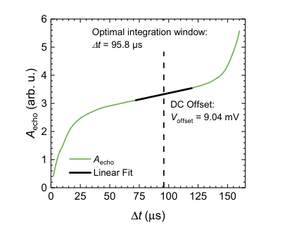
A steep increase for small (large) values of . These are caused by partial integration of the investigated (next) echo peak. In the intermediate region, we observe a linear increase of with . Here, the investigated echo peak is completely inside the integration window and the increase of the echo area is due to the integration of the DC offset. To determine the optimal integration window, we calculate the minimum of the first derivative (dashed line in Figure S4). The DC offset is determined as the slope of a linear fit in the linear regime (solid line in Figure S4).
For the final integration, we subtract the DC offset from the magnitude signal and integrate each detected echo peak using the previously determined integration window.
V Spin-resonator coupling
In this section, we discuss the spin-resonator coupling. The planar resonator structure used in our experiments creates an inhomogenous microwave magnetic field and leads therefore to a distribution of the spin-resonator coupling rate. The analysis of the coupling rate in the presence of an inhomogeneous microwave magnetic field distribution is based on our work described in Ref. [40].

A schematic of the resonator used in the experiment is displayed Fig. S5 (a). The resonator is embedded in the ground plane of a coplanar waveguide (signal line width , gap width ). The resonator is separated from the signal line by a screening line (width ), which defines the external coupling rate [40]. The resonator consists of an inductor (wire width , pitch distance ) with a total length of and a finger capacitor. By changing the length of the capacitor finger the resonance frequency can be tuned.
For a further analysis, we perform finite element simulations using CST Microwave Studio 2016 [41] to extract the three-dimensional microwave magnetic field distributions of the resonator. Figures S5 (b) and (c) show the spatial distribution of the magnitude of the vacuum magnetic field fluctuations , i.e. the field component that is perpendicular to the static magnetic field along the -direction. The data is exported from CST Microwave Studio in volume elements of . The dashed line in panel (c) marks the region where the field amplitude decayed to of the maximum field amplitude. We define this volume as the mode volume of the resonator . Due to the anti-parallel current flow in the inductor wires, the dynamic magnetic field interferes destructively in the far-field. This limits how far the magnetic field reaches into the -direction and enhances the sensitivity of the resonator to spins close to the superconducting resonator.
The single spin-resonator coupling is given by [42]
| (S2) |
where is the electron g-factor of phosphorus donors in silicon [43] and is the Bohr magneton. describes the magnetic field generated by vacuum fluctuations in the resonator. is given by [44] , where is the vacuum permeability, is the reduced Planck constant and is the resonance frequency of the resonator. Collective coupling effects lead to an enhancement of the single-spin coupling rate by a factor , where is the number of spins. Thus, the collective coupling strength is given as
| (S3) |
In this expression, the number of spins, , is replaced by , where is the donor concentration, is the thermal spin polarization and is the sample volume. The filling factor describes the ratio between the sample volume and the mode volume of the resonator.
The planar resonator structures used in this experiment generate an inhomogeneous microwave magnetic field , which has to be taken into account in the filling factor
| (S4) |
We can calculate the filling factor from the exported three-dimensional distribution of the microwave magnetic field using the expression
| (S5) |
With this approach, we obtain a theoretically expected spin-resonator coupling of , which somewhat over-estimates our experimentally defined value. We explain this by a small gap between the resonator and the spin sample [14]. Assuming a gap of , we obtain a quantitative agreement between the theoretically expected spin-resonator coupling and the experimentally determined value of . However, we want to emphasize, that one ingredient for the observation of the phenomenon of a self stimulated echo train is a sufficiently large coupling rate , i.e. placing the system in the strong coupling regime.
Using Eq. S2 we can calculate the distribution of the single spin-resonator coupling . We present the data in Fig. S5 (d) to (f) for different regions above the resonator. Note that we included the finite gap between the resonator and the sample in these calculations. Panel (d) presents the coupling distribution over the entire sample region with a mean coupling strength of (dashed line). This results in a number of spins contributing to the signal according to . For a thin layer of the spin ensemble facing the resonator we compute an enhanced single spin-resonator coupling strength with a mean value of , while spins on the opposite side (panel (f)) couple relatively weakly with on average . The low-frequency peak in the coupling distribution can be attributed to spins outside the resonator dimensions, at the edges of the sample.
VI Estimate of the driven Rabi frequencies and pulse lengths
The finite element simulation of the microwave resonator also allows us to estimate the microwave fields present during the microwave pulses and correspondingly the expected pulse durations for the and pulses. In a simplifying estimate, we can utilize the computed from Fig. S5 to estimate the driven Rabi frequency , as the latter is given by (cf. Eq. S2) [45, 40, 46]. For an initial estimate for , we turn to the Maxwell-Bloch equations and in particular (S13). In detail, we relate the driving amplitude to the experimental microwave power . For a coarse estimate, we further assume a resonant excitation of the microwave resonator with the external microwave tone () and neglect the modifications of the microwave susceptibility of the system stemming from the strong coupling between the spin ensemble to microwave radiation. Note, that these reduce the photon number in a complex fashion, and hence we expect to overestimate our driven Rabi frequency. Using the parameters given in the main text, we find for a peak microwave power of +25dBm at the input of the dilution refrigerator, where we assume that attenuation is solely given by the microwave attenuators presented in Fig. S3 (a total of 70dB attenuation).
In the driven Rabi regime, we next quantitatively estimate by . Using the peak in Fig. S5 (d) at , we obtain corresponding to a -time of . This is a factor of 5 shorter than our experimentally chosen time, however it is worth to point out that this estimate is purely based on the design parameters of the resonator and the attenuators mounted in microwave delivery lines in the setup. Hence, this estimate neglects the additional input losses of the microwave lines, the insertion-loss of the microwave switch and the band pass filter as well as cable connectors, all of which are part of the microwave input circuitry. Those will further reduce the input power supplied to the resonator (we estimate this to be of the order of 5-10dB, corresponding to a reduction in between a factor of roughly 2-3). In addition, this estimate also neglects the modified transmission when the spin ensemble is set in resonance with the microwave resonator. In summary, our crude estimate for the pulse durations for a and pulse agrees well with our selected pulse times. Moreover, this estimate also emphasizes that the pulses have a significant distribution as can be seen in Fig. S5 d).
VII Experimental Pulse optimization
Experimentally, we optimize the pulse angles via the detected echo amplitude. In detail, we vary the pulse length of the first pulse and second pulse until we observe a maximum in the echo amplitude. Although this analysis does not give direct information about the pulse angles of the first and second pulse, we experimentally notice that our pulse settings allow for a partial inversion of the echo, as seen in Sec. X. This observation suggests that we indeed obtain a rotation angle of the order of for our effective -pulse and hence confirms the rotation angles of the order of for our effective -pulse.
VIII Phase cycling experiments
The experimental data in the main text were recorded with a “” pulse sequence, i.e. the two microwave pulses are in phase. We have additionally recorded echo trains where a relative phase shift between the two pulses has been applied. In order to verify the occurence of the echo train phenomenon, a second sample has been used, which is nominally identical to the sample used in the main text. The experiments were performed with the magnetic field centered on the low-field hyperfine transition of the phosphorus donors, which is strongly coupled to the microwave resonator. In Fig. S6, we show the recorded quadratures, and of the microwave transmission signal as a function of time for (a) , (b) ( phase shift), (c) ( phase shift and (d) ( phase shift). In contrast to conventional ESR experiments, where the ESR signal is typically contained in a single phase, in the strong coupling regime the microwave signal is contained in both quadratures. Additionally, no clear phase relation between subsequent echos is observable but rather a phase rotation from one echo to the next. We plot the quadratures of the simulated microwave transmission signal for and in panel (e) and (f), respectively. Our simulations can qualitatively reproduce the complicated phase relation of the echos.
IX Conventional T2 measurements
In a conventional ESR experiment, the coherence time is measured by Hahn echo spectroscopy. A series of Hahn echo pulse sequences consisting of two pulses are performed, where the pulse spacing is varied. The resulting echo appearing after the refocussing pulse is digitized and integrated. The echo area then decreases with the characteristic coherence time in an exponential fashion. We use this experimental approach to determine the coherence time .

In Figure S7, we show such conventional measurements of the spin ensembles in our sample. Panel (a) shows the integrated echo area of the first (conventional) echo of the data presented in Fig. S2 (a). The exponential fit (solid line) results in . As this fit contains only a small number of points due to the limited resolution, we have performed an additional measurement for increased , where we have only digitized the first echo. The evaluation of the time for this measurement presented in panel (b) results in , which is in agreement with the first measurement. In panel (c), we present the same measurement as in (b), with the magnetic field set to the resonance field of the dimer transition. Here, we extract a coherence time . Panel (d) shows the coherence time measurement of the Pb0/Pb1 defects with .
In samples with a large donor concentration as in our case, it is expected that the time is limited by instantaneous diffusion, originating from a dipole-dipole interaction between neighboring spins [47, 48]. The influence of instantaneous diffusion on the time can be reduced by reducing the flipping angle of the second pulse in the Hahn echo [48, 49]. We performed measurements and reduced the amplitude of the second pulse in relation to the amplitude of the first pulse, . We plot the inverse time in Fig. S8. We observe that increases when decreasing the effective flipping angle showing a maximum of . The trend, that smaller rotation angles have a positive effect on is compatible with the mechanism of instantaneous diffusion. Nevertheless, one would expect that the inverse time scales with , where is the rotation angle of the second pulse [50, 51]. However, Fig. S8 does not display this functional behavior, but rather a linear dependence on the pulse amplitude . We speculate, that the details of the complex distribution and the spectral distribution of the spin ensemble might be at the origin of this observed behavior.
The coherence times reported here are exceptionally long compared to conventional pulsed ESR experiments at higher temperatures [48, 49]. We suspect that the long coherence times, which we find already for the initial Hahn-echo sequence, are a result of the suppression of instantaneous diffusion. As reported by Taylor et al. [52], long and weak amplitude pulses cause an effective increase of the time by selecting only a part of the ESR transition and hereby causing a suppression of instantaneous diffusion. In a reference experiment, we performed standard measurement of the coherence time with a Hahn-echo sequence at 6 K (in a commercial Bruker ESR system) and find , which is in good agreement with e.g. Ref. [48].
X T1 measurements
To measure the spin life time we use an inversion recovery pulse sequence [7], as shown in the top of Fig. S9. Conceptually, the first pulse in this three-pulse sequence inverts the spin ensemble. After a variable wait time a standard Hahn echo with fixed is used to probe the magnetization along the -axis, giving a measure of the time.
In Fig. S9 we plot the extracted echo area as a function of the wait time for both the individual P donors and the P2 dimers. Note that the measurements have been recorded at an elevated temperature compared to the measurements in the main text, which, however, has only a small impact on the determined value.
For small , the partially inverted spin ensemble has a net moment along the axis and the resulting echo is negative. Ideally, the inversion pulse should result in a normalized echo amplitude of for , which is not the case here, probably due to the distribution of excitation fields. With increasing spins relax back to thermal equilibrium along and the echo area increases. We fit the following function based on a stretched exponential to the data to extract the time:
| (S6) |
From this fit we extract with for the low-field hyperfine split transition. For the P2 dimers we extract and . A stretched exponential form of the relaxation has been reported, e.g., in NMR for a superposition of single-exponential decays [53]. As the Purcell-enhanced relaxation process depends on the spin-resonator coupling [46], which is highly inhomogeneous in our case, we obtain a distribution of relaxation times, justifying the use of a stretched exponential. Note that we introduce an additional offset in Eq. S6 to account for non-ideal inversion due to the inhomogeneous field distribution. From the ratio of the phosphorus donors, we can estimate that we effectively invert about of the addressed spin ensemble.
We next discuss two mechanisms which could account for these rather short relaxation times: (i) The shortening of the time due to Purcell enhancement and (ii) the one-phonon relaxation process.
Purcell-enhanced T1 times — One mechanism resulting in an enhanced energy relaxation time is Purcell enhancement. This mechanism is present during the free evolution time of the experiment, where each spin individually couples to the microwave resonator. Bienfait et al. [46] discussed this as function of the detuning of the microwave resonator from the spin systems and find for bismuth donors in silicon shortened relaxation times in the seconds range. Following their discussion, we can calculate the Purcell rate by
| (S7) |
where we have replaced the FWHM of Ref.[46] with our HWHM . Using the peak in depicted in Fig. S5 (d) and of the main text, we expect a Purcell-limited time of . However, we also find a considerable amount of spins with a spin-resonator coupling of , which would translate to a time of . We speculate that spatial diffusion [54, 55, 56, 57] can then assist with the relaxation of the majority of spins in the mode volume. However, tailored experiments, which are beyond the scope of this work, will be required to test this conjecture.
One-phonon relaxation process — In addition, we can consider the process originating from the relaxation with the phonons. As our experiments are performed at low temperatures, we can reduce the discussion to the one-phonon relaxation process [58]. Morello et al. [59] discussed this process, which was initially presented by Hasegawa et al. [60] in the low temperature limit. Both report for a temperature and magnetic field dependence of the spin lattice relaxation rate of
| (S8) |
To discuss the phonon related relaxation process at even lower temperatures, we need to account for the phonon population, which is given by the Bose-factor [60]. Then
| (S9) |
For , this simplifies to the expected dependence, while for we find the limit of . Using the reported spin relaxation time by Feher and Gere [58] for our donor concentration of of at as a calibration point, we can now extrapolate to our experimental temperature and . We find . We note that this relatively short time is mostly caused by the high doping concentration.
In summary, both presented relaxation mechanisms reasonably explain our measured spin relaxation times .
In addition, we can use these estimates to calculate the expected spectral diffusion rate, which might mask the measurement and has potentially impact on the experimentally determined times presented in this paper. Spectral diffusion depends on the donor concentration and the corresponding time constant is given by [51]
| (S10) |
Using the times determined above of and , we expect spectral diffusion rates of and , respectively. For our experimentally determined time of we obtain . All of these estimates for exceed the observed times significantly and hence we expect that our measurements are not dominated by this mechanism. As the spin relaxation time represents an important parameter, we plan to investigate aspects of spin relaxation in these strongly coupled systems at a later stage in more detail using pulse sequences based on adiabatic pulses, optimal control pulses or a two-pulse saturation recovery, which have the potential to discern spectral diffusion from spin relaxation, excitation of a selected part of the spin ensemble and Purcell rates.
XI Theoretical model
In order to give a dynamical description of the echo trains we start from the inhomogeneous Tavis-Cummings Hamiltonian [61],
| (S11) | |||||
where and are the detunings of the resonator frequency and of the individual spin frequencies from the frequency of the incoming driving pulse. Here and are the creation and annihilation operators of the single resonator mode and , , and are the Pauli operators corresponding to the individual spins. Without loss of generality we assume as well as . The incoming driving pulse is characterized by the carrier frequency and the amplitude , which for simplicity is assumed to be of rectangular shape. Note that the Hamiltonian (S11) does not account for direct dipole-dipole interactions between the spins. Although dipole-dipole interactions do not seem to play a fundamental role in the formation of the echo pulses it would be interesting to investigate in future studies whether they have an impact on the shape of the echos.
A quantum master equation for the system’s density matrix can be written as [62], where is the Hamiltonian (S11) and stands for the standard Lindblad superoperator
| (S12) |
Here the first term describes the resonator losses with the decay rate and the second and third term account for nonradiative and radiative dephasing of the individual spins characterized by the rates and , respectively. Starting from the master equation given above, one can derive the equations of motion for the expectation value of any operator by . In the limit of very large spin ensembles (), we can neglect correlations between the resonator field and individual spins () [37]. Thus, we obtain a closed set of first-order differential equations for the expectation values , , and , which is equivalent to the well-known Maxwell-Bloch equations:
| (S13) | ||||
| (S14) | ||||
| (S15) |
with the resonator decay rate , the longitudinal spin relaxation rate , and transverse spin relaxation rate .
As outlined in the main text, the spin ensemble is inhomogeneously broadened not only with regard to the individual spin frequencies , but also through the coupling strengths due to the inhomogeneity. Since we are dealing with a sizable number of spins () inside the ensemble, the distributions of spin frequencies and couplings strengths are smooth functions around the mean values. For simplicity, we assume in our calculations that all spins couple with the mean coupling strength and we incorporate the inhomogeneaus broadening in a phenomenological Lorentzian spin spectral density
| (S16) |
This frequency distribution of spins is already sufficient to accurately describe the generation of multiple echo trains. Here is the half width at half maximum and is the mean frequency of the spin distribution.
To solve (S13)-(S15) for the inhomogeneously broadened spin ensemble, we discretize the phenomenological spin spectral density and divide the entire frequency range into equidistant frequency clusters. Each cluster is then characterized by the mean coupling strength , its detuning , and the number of spins inside this cluster. Eqs. S13-S15 can then be solved using a standard Runge-Kutta method.
Note that, along the lines of previous work [22, 38], the distribution of coupling strengths can also be included in the phenomenological spin spectral density. Calculations using such a combined spin spectral density have also been carried out and showed qualitatively similar results. In order to obtain a full quantitative agreement between our theory and the experiment, however, the exact shape of the spectral spin and spatial coupling distribution has to be determined through extensive further theoretical and experimental work [63]. For reasons of clarity, we only present simulations in which the inhomogeneous broadening is included in the spin distribution alone, since these are already sufficient to describe the observed phenomenon of multiple echoes.
XII A short review on multiple echo effects
Multiple echo effects in nuclear and electron magnetic resonance (NMR, ESR) experiments have been observed in a number of experiments, although different underlying mechanism are presented. Multiple echo signatures were reported in NMR experiments of 3He, 3He/4He mixtures as well as water [64, 65, 66, 67]. In these experiments the occurrence of multiple echos is attributed to non-linear terms in the equation of motion governing the magnetization. In Fermi liquids, the non-linearity is introduced by the Leggett-Rice effect [66, 68]. Neither effect plays a role in our experiments. Another source for non-linear terms in the Bloch equations is the dipolar demagnetizing field [68]. The demagnetizing field is usually negligible NMR and ESR experiments, as it is suppressed by radiation damping [69, 70]. However, in the experiments presented in Ref. [69, 70] a strong field gradient parallel to the static magnetic field was applied, which crucially alters the effect of the demagnetizing field on the dynamics [70]. Another source of nonlinear spin dynamics is radiation damping [71, 72]. Radiation damping describes the effects of a backaction of the precessing spin magnetization on the RF coil or resonator, sharing some similarities with the strong coupling regime. Numerical simulations of the nonlinear Maxwell-Bloch equations indeed show the presence of multiple echos under certain conditions [73].
The first occurrence of a multiple echo signal in ESR was reported by Gordon and Bowers [24]. Here, the authors conducted Hahn echo experiments of donors in silicon at a frequency of . We are able to estimate the relevant coupling parameters from the information supplied in the text: Assuming a typical TE102 cavity for operation at and a sample volume of , we estimate a filling factor of . We calculate the effective coupling rate using Eq. (S3) and a donor concentration of and obtain . With the spin relaxation rate and the assumption of a moderate quality factor of , we estimate a cooperativity of . Therefore, the occurrence of the second echo reported in Ref. [24] can be in hindsight explained by our model.