跳到论文正文
W Papers独立论文阅读器 arXiv:1809.09669 论文正文 计算阅读时间 · 0%
引用这篇论文根据当前论文元数据生成,正式投稿前建议核对。


License: arXiv.org perpetual non-exclusive license
arXiv:1809.09669v1 [math.NA] 25 Sep 2018

Scattering problems from slightly perturbed periodic surfaces: Part II. High order numerical method

Ruming Zhang ††thanks: Center for Industrial Mathematics, University of Bremen; rzhang@uni-bremen.de
Abstract

In this paper, we develop a high order numerical method for the numerical solutions of scattering problems with slightly perturbed periodic surfaces in two dimensional spaces. Based on the regularity property introduced in Part I, the decaying rate of the incident field could be transferred directly to the total field for small perturbations. Thus the finite section method could reach a high accuracy rate. With the help of a modification of the truncated problem, the problem is solved by a finite element method. The convergence of the finite element method is proved and numerical examples have been carried out to show the efficiency of the numerical scheme.

1 Introduction

Numerical simulations of scattering problems with rough surfaces are always challenging. The unbounded domain always needs to be truncated, and the error caused by the truncation depends greatly on the properties of the total fields. This paper considers a special family of rough surface scattering problems, i.e., when the incident field satisfies certain conditions and the rough surface is a slightly perturbation of a periodic one.

Generally speaking, the slightly perturbed periodic surfaces could be treated as rough surfaces if the periodicities are ignored, thus there are some known method for the theoretical and numerical analysis of these problems. We refer to [CWZ96, CWRZ99, ZCW03, CWHP06] for the integral equation method. An alternative way is to apply the variational method, see [CM05, CE10]. The numerical methods for the rough surface scattering problems are always based on the decaying property of the total field (see [MACK00, MC01] for the numerical solutions of the integral equations and [CE10] for the finite section method). Due to the limited decaying rate, the finite section method always converges slowly.

Until recent years, theoretical and numerical analysis based on the Floquet-Bloch transform provide another way to deal with these problems. With the help of this method, a couple of scattering problems with (locally perturbed) periodic background have been studied and efficient numerical methods have been developed. We would like to mention [Coa12, HN16] for the scattering problems from locally perturbed periodic media. With a domain transformation technique, the Bloch transform was applied to the scattering problems with locally perturbed periodic surfaces in [Lec17]. Based on that, numerical methods have been developed, for 2D cases see [LZ17a, LZ17b] and for 3D cases see [LZ17c]. The method has also been extended to globally perturbed problems, see [Zha18a, Zha18c]. On the other hand, a high order numerical method has also been developed, see [Zha18b]. It was also shown that, the smoothness of the Bloch transformed field with respect to the quasi-periodicity parameter depends on the incident field, except for the square-root like singularities brought by the Dirichlet-to-Neumann map.

The paper [Zha18d] considers the scattering problems with globally perturbed periodic surfaces. It is proved that, when the incident field satisfies special conditions and the perturbation of the periodic surface is small enough, the regularity of the Bloch transformed field with respect to the quasi-periodicity parameter only depends on the incident field. This result provides a possibility to develop an efficient numerical method when the incident field is smooth enough. The problem is modified into an equivalent one due to the singularity of the Dirichlet-to-Neumann map, and the well-posedness of the new problem comes directly from the equivalence. The next step is to truncate the term defined in the unbounded domain. A high order convergence rate comes from the high regularity of the Bloch transformed field. Then a classical finite element method is adopted, and the convergence is proved for the numerical method.

The rest of this paper is organized as follows. In Section 2, we briefly recall the mathematical modal and well-posedness of the rough surface scattering problems, and the properties of the Bloch transformed problems. The third section recalls the regularity result from [Zha18d]. In the fourth section, we show the classic finite element method introduced in [LZ17b] and its disadvantages. The fifth section shows the modified variational problems, with the help of change of variables. In the sixth section, we apply the finite section method for the truncation of the unbounded term, and estimate the error of the truncation. In the seventh section, we apply the finite element method to the truncation of the modified variational problem. In the last section, the numerical experiments are carried out to show the efficiency of the numerical scheme.

2 Scattering problems from slightly perturbed periodic surfaces

2.1 Mathematical model and well-posedness

In this section, the mathematical formulation of the scattering problems in two dimensional spaces is presented. For details we refer to [CM05, CE10].

Refer to caption
Figure 1: Red curve: periodic surface; black curve: slightly perturbed periodic surface.

Let ζ\zeta be a bounded function defined in ℝ\mathbb{R}, and the surface Γ⊂ℝ2\Gamma\subset\mathbb{R}^{2} is defined by

Γ:={x∈ℝ2:x2=ζ⁡(x1)​ where ​x1∈ℝ}.\Gamma:=\big\{x\in\mathbb{R}^{2}:\,x_{2}=\zeta(x_{1})\text{ where }x_{1}\in\mathbb{R}\big\}.

The domain above the surface is defined by

Ω:={x∈ℝ2:x2>ζ⁡(x1)}.\Omega:=\left\{x\in\mathbb{R}^{2}:\,x_{2}>\zeta(x_{1})\right\}.

Suppose HH is a constant satisfies H>maxt∈ℝ⁡{ζ⁡(t)}H>\max_{t\in\mathbb{R}}\left\{\zeta(t)\right\}, then ΓH:=ℝ×{H}\Gamma_{H}:=\mathbb{R}\times\{H\} is a straight line lies above Γ\Gamma. Define the domain above Γ\Gamma. Define the domain with finite height:

ΩH:={x∈ℝ2:ζ⁡(x1)<x2<H}.\Omega_{H}:=\left\{x\in\mathbb{R}^{2}:\,\zeta(x_{1})<x_{2}<H\right\}.

We consider the following equations in ΩH\Omega_{H}:

Δ​u+k2​u=0 in ​ΩH;\displaystyle\Delta u+k^{2}u=0\quad\text{ in }\Omega_{H}; (1)
u=0 on ​Γ;\displaystyle u=0\quad\text{ on }\Gamma; (2)
∂u∂xd​(x~,H)=T+​[u|ΓH]+f on ​ΓH,\displaystyle\frac{\partial u}{\partial x_{d}}(\widetilde{x},H)=T^{+}\left[u\big|_{\Gamma_{H}}\right]+f\quad\text{ on }\Gamma_{H}, (3)

where T+T^{+} is the Dirichlet-to-Neumann map defined by

T+​φ=i2​π​∫ℝk2−|ξ|s​ei​x1⋅ξ​φ^​(ξ)​𝑑ξ for ​φ=12​π​∫ℝei​x1⋅ξ​φ^​(ξ)​𝑑ξ,T^{+}\varphi=\frac{\mathrm{i}}{{2\pi}}\int_{\mathbb{R}}\sqrt{k^{2}-|{\xi}|^{s}}e^{\mathrm{i}x_{1}\cdot{\xi}}\widehat{\varphi}({\xi})\,\mathrm{d}\xi\,\quad\text{ for }\varphi=\frac{1}{2\pi}\int_{\mathbb{R}}e^{\mathrm{i}x_{1}\cdot{\xi}}\widehat{\varphi}({\xi})\,\mathrm{d}\xi\,, (4)

and ff is defined by

f:=∂ui∂x2​(x1,H)−T+​[ui|ΓH]f:=\frac{\partial u^{i}}{\partial x_{2}}(x_{1},H)-T^{+}\left[u^{i}|_{\Gamma_{H}}\right] (5)

for the incident field uiu^{i} that satisfies the Helmholtz equation in Ω\Omega.

The weak formulation for the scattering problem is, given any ff in the weighted Sobolev space Hr−1/2(ΓH)H_{r}^{-1/2}(\Gamma_{H}), to find a solution u∈H~r1​(ΩH)u\in\widetilde{H}_{r}^{1}(\Omega_{H}) such that

∫ΩH[∇u⋅∇v¯−k2​u​v¯]​𝑑x−∫ΓHT+​[u|ΓH]​v¯​𝑑s=∫ΓHf​v¯​𝑑s,\int_{\Omega_{H}}\left[\nabla u\cdot\nabla\overline{v}-k^{2}u\overline{v}\right]\,\mathrm{d}x\,-\int_{\Gamma_{H}}T^{+}\left[u|_{\Gamma_{H}}\right]\overline{v}\,\mathrm{d}s\,=\int_{\Gamma_{H}}f\overline{v}\,\mathrm{d}s\,, (6)

for all v∈H~r1​(ΩH)v\in\widetilde{H}^{1}_{r}(\Omega_{H}) with compact support in ΩH¯\overline{\Omega_{H}}.

Remark 1.

The tilde in H~r1​(ΩH)\widetilde{H}_{r}^{1}(\Omega_{H}) shows that the functions in this space belong to Hr1​(ΩH)H_{r}^{1}(\Omega_{H}) and satisfy homogeneous Dirichlet boundary condition on Γ\Gamma. Similar notations are utilized for other spaces, e.g., H0r​(WΛ∗,H~αs​(ΩHΛ))H_{0}^{r}({W_{\hskip-1.0pt{\Lambda}^{\ast}}};\widetilde{H}_{\alpha}^{s}(\Omega^{\Lambda}_{H})).

From [CE10], the unique solvability of the variational problem 6 has been proved in weighted Sobolev spaces.

Theorem 2.

If Γ\Gamma is Lipschitz continuous, f∈Hr−1/2(ΓH)f\in H_{r}^{-1/2}(\Gamma_{H}) for |r|<1|r|<1, then there is a unique solution u∈H~r1​(ΩH)u\in\widetilde{H}_{r}^{1}(\Omega_{H}) for the variational problem (6).

2.2 The Bloch transformed problem

In this subsection, we apply the Bloch transform to the scattering problems. Suppose Λ>0\Lambda>0 and the surface ζ\zeta is Λ\Lambda-periodic, and let the function ζp\zeta_{p} be a global perturbation of ζ\zeta. Let the surface defined by ζp\zeta_{p} be denoted by Γp\Gamma_{p}, and the domains Ωp\Omega^{p} and ΩHp\Omega^{p}_{H} are defined in the same way.

Let Λ∗:=2​π/Λ\Lambda^{*}:=2\pi/\Lambda, define the periodic cell and dual cell by

WΛ:=(−Λ2,Λ2];WΛ∗:=(−Λ∗2,Λ∗2]=(−πΛ,πΛ].{W_{\hskip-1.0pt{\Lambda}}}:=\left(-\frac{\Lambda}{2},\frac{\Lambda}{2}\right];\quad{W_{\hskip-1.0pt{\Lambda}^{\ast}}}:=\left(-\frac{\Lambda^{*}}{2},\frac{\Lambda^{*}}{2}\right]=\left(-\frac{\pi}{\Lambda},\frac{\pi}{\Lambda}\right].

Now we can define ΓHΛ\Gamma^{\Lambda}_{H} and ΩHΛ\Omega^{\Lambda}_{H}, which are ΓH\Gamma_{H} and ΩH\Omega_{H} restricted in one periodic cell WΛ×ℝ{W_{\hskip-1.0pt{\Lambda}}}\times\mathbb{R}, i.e.,

ΓHΛ=ΓH∩[WΛ×ℝ],ΩHΛ=ΩH∩[WΛ×ℝ].\Gamma^{\Lambda}_{H}=\Gamma_{H}\cap\left[{W_{\hskip-1.0pt{\Lambda}}}\times\mathbb{R}\right],\quad\Omega^{\Lambda}_{H}=\Omega_{H}\cap\left[{W_{\hskip-1.0pt{\Lambda}}}\times\mathbb{R}\right].

Let Θp\Theta_{p} be a diffeomorphism that maps ΩH0p\Omega^{p}_{H_{0}} to ΩH0\Omega_{H_{0}} for some ‖ζ‖∞<H0<H\|\zeta\|_{\infty}<H_{0}<H, and extend Θp\Theta_{p} by identity in ℝ×[H0,∞)\mathbb{R}\times[H_{0},\infty). Thus the support of Θp−I\Theta_{p}-I is contained in ΩH0\Omega_{H_{0}}. Let the transformed total field uT:=u∘Θpu_{T}:=u\,\circ\,\Theta_{p}, then by direct calculation, uT∈H~r1​(ΩH)u_{T}\in\widetilde{H}_{r}^{1}(\Omega_{H}) satisfies the following variational problem in the periodic domain ΩH\Omega_{H}

∫ΩH[Ap∇uT⋅∇vT¯−k2cpuTvT¯]dx−∫ΓHT+[uT|ΓH]vT¯ds=∫ΓHfvT¯ds,\int_{\Omega_{H}}\left[A_{p}\nabla u_{T}\cdot\nabla\overline{v_{T}}-k^{2}c_{p}u_{T}\overline{v_{T}}\right]\,\mathrm{d}x\,-\int_{\Gamma_{H}}T^{+}\left[u_{T}|_{\Gamma_{H}}\right]\overline{v_{T}}\,\mathrm{d}s\,=\int_{\Gamma_{H}}f\overline{v_{T}}\,\mathrm{d}s\,, (7)

for all vT:=v∘Θ∈H~1​(ΩH)v_{T}:=v\circ\Theta\in\widetilde{H}^{1}(\Omega_{H}), where

Ap​(x):=|det∇Θp​(x)|​[(∇Θp​(x))−1​(∇Θp​(x))−T]∈L∞​(ΩH,ℝ2×2);\displaystyle A_{p}({x}):=\left|\det\nabla\Theta_{p}({x})\right|\left[\left(\nabla\Theta_{p}({x})\right)^{-1}\left(\nabla\Theta_{p}({x})\right)^{-T}\right]\in L^{\infty}\left(\Omega_{H},\mathbb{R}^{2\times 2}\right);
cp​(x):=|det∇Θp​(x)|∈L∞​(ΩH).\displaystyle c_{p}(x):=\left|\det\nabla\Theta_{p}({x})\right|\in L^{\infty}(\Omega_{H}).

Thus the supports of both Ap−I2A_{p}-I_{2} and cp−1c_{p}-1 are subsets of ΩH0\Omega_{H_{0}}.

Apply the the Bloch transform to (7), we arrive at the variational problem for w=𝒥ΩH​uTw=\mathcal{J}_{\Omega_{H}}u_{T} with test function z=𝒥ΩH​vTz={\mathcal{J}_{\Omega_{H}}{v_{T}}}:

∫WΛ∗aα​(w⁡(α,⋅),z⁡(α,⋅))​𝑑α+b⁡(w,z)=∫WΛ∗∫ΓHΛF⁡(α,x)​z⁡(α,x)¯​𝑑s​(x)​𝑑α,\int_{W_{\hskip-1.0pt{\Lambda}^{\ast}}}a_{\alpha}(w(\alpha,\cdot),z(\alpha,\cdot))\,\mathrm{d}\alpha\,+\,b(w,z)=\int_{W_{\hskip-1.0pt{\Lambda}^{\ast}}}\int_{\Gamma^{\Lambda}_{H}}F(\alpha,x)\overline{z(\alpha,x)}\,\mathrm{d}s(x)\,\,\mathrm{d}\alpha\,, (8)

where

aα​(w,z):=∫ΩHΛ[∇w⋅∇z¯−k2​w​z¯]​𝑑x−∫ΓHΛTα+​(w)​z¯​𝑑s,\displaystyle a_{\alpha}(w,z):=\int_{\Omega^{\Lambda}_{H}}\left[\nabla w\cdot\nabla\overline{z}-k^{2}w\overline{z}\right]\,\mathrm{d}x\,-\int_{\Gamma^{\Lambda}_{H}}T^{+}_{\alpha}(w)\overline{z}\,\mathrm{d}s\,,
b⁡(w,z)=∫ΩH[(Ap−I2)∇(𝒥ΩH−1w)⋅∇(𝒥ΩH−1​z)¯−k2(cp−1)(𝒥ΩH−1w)⋅(𝒥ΩH−1​z)¯]dx,=∫WΛ∗∫ΩHΛ[𝒥ΩH[(Ap−I2)∇(𝒥ΩH−1w)⋅∇z¯−k2𝒥ΩH[(cp−1)(𝒥ΩH−1w)]z¯]]dxdα,\displaystyle\begin{aligned} b(w,z)&=\int_{\Omega_{H}}\Big[(A_{p}-I_{2})\nabla(\mathcal{J}_{\Omega_{H}}^{-1}w)\cdot\nabla\overline{\left(\mathcal{J}_{\Omega_{H}}^{-1}{z}\right)}-k^{2}(c_{p}-1)(\mathcal{J}_{\Omega_{H}}^{-1}w)\cdot\overline{\left(\mathcal{J}_{\Omega_{H}}^{-1}{z}\right)}\Big]\,\mathrm{d}x\,,\\ &=\int_{W_{\hskip-1.0pt{\Lambda}^{\ast}}}\int_{\Omega^{\Lambda}_{H}}\left[\mathcal{J}_{\Omega_{H}}\left[(A_{p}-I_{2})\nabla(\mathcal{J}_{\Omega_{H}}^{-1}w)\cdot\nabla\overline{z}-k^{2}\mathcal{J}_{\Omega_{H}}\left[(c_{p}-1)(\mathcal{J}_{\Omega_{H}}^{-1}w)\right]\overline{z}\right]\right]\,\mathrm{d}x\,\,\mathrm{d}\alpha\,,\end{aligned}
F⁡(α,x)=(𝒥ΓH​f)​(α,x).\displaystyle F(\alpha,x)=\left(\mathcal{J}_{\Gamma_{H}}f\right)(\alpha,x).

Moreover, the operator Tα+T^{+}_{\alpha} is the well-known α{\alpha}-quasi-periodic Dirichlet-to-Neumann operator from Hα1/2​(ΓH)H^{1/2}_{\alpha}(\Gamma_{H}) to Hα−1/2(ΓH)H^{-1/2}_{\alpha}(\Gamma_{H}) defined by

Tα+​φ=i​∑j∈ℤd−1k2−|Λ∗​j−α|2​φ^​(j)​ei⁡(Λ∗​j−α)⋅x~ for ​φ=∑j∈ℤd−1φ^​(j)​ei⁡(Λ∗​j−α)⋅x~.T_{\alpha}^{+}\varphi=\mathrm{i}\sum_{{j}\in\mathbb{Z}^{d-1}}\sqrt{k^{2}-|\Lambda^{*}j-{\alpha}|^{2}}\widehat{\varphi}({j})e^{\mathrm{i}(\Lambda^{*}{j}-{\alpha})\cdot\widetilde{x}}\quad\text{ for }\varphi=\sum_{{j}\in\mathbb{Z}^{d-1}}\widehat{\varphi}({j})e^{\mathrm{i}(\Lambda^{*}{j}-{\alpha})\cdot\widetilde{x}}.

The equivalence, well-posedness and regularity results are easily extended from locally perturbed cases (see [Lec17, LZ17b]), and the results have been proved in [Zha18a], and we list these results in the following theorem.

Theorem 3 (Lemma 7, Theorem 8-10, [Zha18a]).

Assume that f∈Hr−1/2(ΓH)f\in H_{r}^{-1/2}(\Gamma_{H}) for r∈(0,1)r\in(0,1) and ζ,ζp\zeta,\,\zeta_{p} are Lipschitz continuous functions.

  1. 1.

    u∈H~r1​(ΩH)u\in\widetilde{H}^{1}_{r}(\Omega_{H}) satisfies (6) if and only if w=𝒥ΩH​uT∈H0r​(WΛ∗,H~α1​(ΩHΛ))w=\mathcal{J}_{\Omega_{H}}u_{T}\in H_{0}^{r}({W_{\hskip-1.0pt{\Lambda}^{\ast}}};\widetilde{H}^{1}_{\alpha}(\Omega^{\Lambda}_{H})) satisfies (8) with F⁡(α,⋅)=𝒥ΩH​fF(\alpha,\cdot)=\mathcal{J}_{\Omega_{H}}f.

  2. 2.

    Given any F∈H0r(WΛ∗;Hα−1/2(ΓHΛ))F\in H_{0}^{r}({W_{\hskip-1.0pt{\Lambda}^{\ast}}};H_{\alpha}^{-1/2}(\Gamma_{H}^{\Lambda})) for some r∈[0,1)r\in[0,1), the variational problem (8) has a unique solution in H0r​(WΛ∗,H~α1​(ΩHΛ))H_{0}^{r}({W_{\hskip-1.0pt{\Lambda}^{\ast}}};\widetilde{H}^{1}_{\alpha}(\Omega^{\Lambda}_{H})).

  3. 3.

    If f∈Hr1/2​(ΓH)f\in H_{r}^{1/2}(\Gamma_{H}) and ζ∈C2,1​(ℝ)\zeta\in C^{2,1}(\mathbb{R}), the solution w∈H0r​(WΛ∗,H~α2​(ΩHΛ))w\in H_{0}^{r}({W_{\hskip-1.0pt{\Lambda}^{\ast}}};\widetilde{H}^{2}_{\alpha}(\Omega^{\Lambda}_{H})).

  4. 4.

    If r∈(1/2,1)r\in(1/2,1), then the solution w∈H0r​(WΛ∗,H~α1​(ΩHΛ))w\in H_{0}^{r}({W_{\hskip-1.0pt{\Lambda}^{\ast}}};\widetilde{H}^{1}_{\alpha}(\Omega^{\Lambda}_{H})) equivalently satisfies for all α∈WΛ∗\alpha\in{W_{\hskip-1.0pt{\Lambda}^{\ast}}} and zα∈H~α1​(ΩHΛ)z_{\alpha}\in\widetilde{H}_{\alpha}^{1}(\Omega^{\Lambda}_{H}) such that

    aα​(w⁡(α,⋅),zα)+b⁡(w⁡(α,⋅),zα)=∫ΓHΛF⁡(α,x)​zα​(x)¯​𝑑s​(x).a_{\alpha}(w(\alpha,\cdot),z_{\alpha})+b(w(\alpha,\cdot),z_{\alpha})=\int_{\Gamma^{\Lambda}_{H}}F(\alpha,x)\overline{z_{\alpha}(x)}\,\mathrm{d}s\,(x). (9)

3 Regularity in Sobolev spaces

3.1 High order regularity

In this section, we conclude some regularity properties of the Bloch transformed scattering problems from locally or globally perturbed periodic surfaces obtained in [Zha18d]. The result from [CE10], only for |r|<1|r|<1, the decaying rate of the incident field could be transferred to the total field. However, for some special cases, the result holds for r≥1r\geq 1 (see [Zha18d]). In the following, we will consider these special cases and list the known results obtained in [Zha18b, Zha18d].

For convenience, we define the discrete set that depends on kk and Λ∗\Lambda^{*}:

𝒮:={α0∈WΛ∗¯:∃j∈ℤ​ such that ​|Λ∗​j−α0|=k}.\mathcal{S}:=\big\{\alpha_{0}\in\overline{{W_{\hskip-1.0pt{\Lambda}^{\ast}}}}:\,\exists\,j\in\mathbb{Z}\text{ such that }|\Lambda^{*}j-\alpha_{0}|=k\big\}. (10)

It is a non-empty discrete set that has at most three points. From the analysis in [Zha18b], there are two different kinds of wave numbers that correspond to two kinds of representations of 𝒮\mathcal{S}. Define the real number k¯\underline{k} by

k¯:=min⁡{|Λ∗​j−k|:j∈ℤ},\underline{k}:=\min\{|\Lambda^{*}j-k|:\,j\in\mathbb{Z}\}, (11)

then 0≤k¯≤Λ∗/20\leq\underline{k}\leq\Lambda^{*}/2 and the points in 𝒮\mathcal{S} could be represented by k¯\underline{k}:

  • •

    Case 1, k¯=m​Λ∗/2\underline{k}=m\Lambda^{*}/2 for some m=0,1m=0,1, then 𝒮={k¯+Λ∗​j:j∈ℤ}∩WΛ∗¯\mathcal{S}=\{\underline{k}+\Lambda^{*}j:\,j\in\mathbb{Z}\}\cap\overline{{W_{\hskip-1.0pt{\Lambda}^{\ast}}}};

  • •

    Case 2, k¯≠m​Λ∗/2\underline{k}\neq m\Lambda^{*}/2 for any m=0,1m=0,1, then 𝒮={k¯+Λ∗j,−k¯+Λ∗j:j∈ℤ}∩WΛ∗¯\mathcal{S}=\{\underline{k}+\Lambda^{*}j,\,-\underline{k}+\Lambda^{*}j:\,j\in\mathbb{Z}\}\cap\overline{{W_{\hskip-1.0pt{\Lambda}^{\ast}}}}.

As was shown in [Zha18d], the points in 𝒮\mathcal{S} are critical, as the α\alpha-dependent quasi-periodic Dirichlet-to-Neumann map Tα+T^{+}_{\alpha} has a square-root like singularity in the neighbourhood of these points.

In [Zha18d], when the right hand side belongs to a closed subspace of H0n​(WΛ∗,H~α1​(ΓHΛ))H_{0}^{n}({W_{\hskip-1.0pt{\Lambda}^{\ast}}};\widetilde{H}^{1}_{\alpha}(\Gamma^{\Lambda}_{H})) for some n∈ℕn\in\mathbb{N}, the regularity of the solutions of (8) with respect to α\alpha only depends on rr.

Refer to caption
Figure 2: Distribution of the set 𝒮\mathcal{S} for Λ=2​π\Lambda=2\pi. Left: k=1.5k=1.5; right: k=2k=\sqrt{2}. WΛ∗{W_{\hskip-1.0pt{\Lambda}^{\ast}}} is the line ℝ×{0}\mathbb{R}\times\{0\} between the black dotted lines.

The first theorem considers Bloch transformed problem (8), when the perturbation of the periodic is small enough. First, we introduce the space H00n​(WΛ∗,𝒮,H~α1​(ΩHΛ))H_{00}^{n}({W_{\hskip-1.0pt{\Lambda}^{\ast}}};\mathcal{S};\widetilde{H}^{1}_{\alpha}(\Omega^{\Lambda}_{H})) by the closure of the set

{φ∈C∞(WΛ∗×ΩHΛ):∃δ>0,s.t.,φ(α,⋅)=0 for α∈⋃α0∈𝒮B(α0,δ)∩WΛ∗}\left\{\varphi\in C^{\infty}({W_{\hskip-1.0pt{\Lambda}^{\ast}}}\times\Omega^{\Lambda}_{H}):\,\exists\delta>0,s.t.,\varphi(\alpha,\cdot)=0\text{ for }\alpha\in\bigcup_{\alpha_{0}\in\mathcal{S}}B(\alpha_{0},\delta)\cap{W_{\hskip-1.0pt{\Lambda}^{\ast}}}\right\} (12)

with respect to the H0n​(WΛ∗,Hαs​(ΩHΛ))H_{0}^{n}({W_{\hskip-1.0pt{\Lambda}^{\ast}}};H^{s}_{\alpha}(\Omega^{\Lambda}_{H}))-norm, where B⁡(α0,δ)=(α0−δ,α0+δ)B(\alpha_{0},\delta)=(\alpha_{0}-\delta,\alpha_{0}+\delta).

Theorem 4 (Theorem 24, [Zha18d]).

Suppose ζ,ζp\zeta,\,\zeta_{p} are Lipschitz continuous functions. ζ\zeta is Λ\Lambda-periodic and ζp\zeta_{p} is a slight perturbation of ζ\zeta. If F∈H00n(WΛ∗;𝒮;Hα−1/2(ΓHΛ))F\in H_{00}^{n}({W_{\hskip-1.0pt{\Lambda}^{\ast}}};\mathcal{S};H^{-1/2}_{\alpha}(\Gamma^{\Lambda}_{H})) for some n∈ℕn\in\mathbb{N}, then w∈H0n​(WΛ∗,H~α1​(ΩHΛ))w\in H_{0}^{n}({W_{\hskip-1.0pt{\Lambda}^{\ast}}};\widetilde{H}^{1}_{\alpha}(\Omega^{\Lambda}_{H})).

For simplicity, we adopt notations from [Zha18d]. From Riesz representation theorem, there are operators 𝒜,ℬp∈ℒ⁡(L2​(WΛ∗,H~α1​(ΩHΛ))){\mathcal{A}},\,{\mathcal{B}}_{p}\in\mathcal{L}(L^{2}({W_{\hskip-1.0pt{\Lambda}^{\ast}}};\widetilde{H}^{1}_{\alpha}(\Omega^{\Lambda}_{H}))) that satisfies

⟨𝒜​w,z⟩=∫WΛ∗aα​(w⁡(α,⋅),z⁡(α,⋅))​𝑑α;⟨ℬp​w,z⟩=b⁡(w,z)\left<{\mathcal{A}}w,z\right>=\int_{W_{\hskip-1.0pt{\Lambda}^{\ast}}}a_{\alpha}(w(\alpha,\cdot),z(\alpha,\cdot))\,\mathrm{d}\alpha\,;\quad\left<{\mathcal{B}}_{p}w,z\right>=b(w,z) (13)

for any w,z∈L2​(WΛ∗,H~α1​(ΩHΛ))w,z\in L^{2}({W_{\hskip-1.0pt{\Lambda}^{\ast}}};\widetilde{H}^{1}_{\alpha}(\Omega^{\Lambda}_{H})), where ⟨⋅,⋅⟩\left<\cdot,\cdot\right> is the inner product in the space L2​(WΛ∗,H~α1​(ΩHΛ))L^{2}({W_{\hskip-1.0pt{\Lambda}^{\ast}}};\widetilde{H}^{1}_{\alpha}(\Omega^{\Lambda}_{H})). Use Riesz representation theorem again, there is a G∈H00n​(WΛ∗,𝒮,H~α1​(ΩHΛ))G\in H_{00}^{n}({W_{\hskip-1.0pt{\Lambda}^{\ast}}};\mathcal{S};\widetilde{H}^{1}_{\alpha}(\Omega^{\Lambda}_{H})) such that

∫WΛ∗∫ΓHΛF⁡(α,x)​z⁡(α,x)¯​𝑑x​𝑑α=⟨G,z⟩.\int_{W_{\hskip-1.0pt{\Lambda}^{\ast}}}\int_{\Gamma^{\Lambda}_{H}}F(\alpha,x)\overline{z(\alpha,x)}\,\mathrm{d}x\,\,\mathrm{d}\alpha\,=\left<G,z\right>. (14)

Theorem 24, [Zha18d], that 𝒜+ℬp{\mathcal{A}}+{\mathcal{B}}_{p} is invertible in H00n​(WΛ∗,𝒮,H~α1​(ΩHΛ))H_{00}^{n}({W_{\hskip-1.0pt{\Lambda}^{\ast}}};\mathcal{S};\widetilde{H}^{1}_{\alpha}(\Omega^{\Lambda}_{H})), and for any G∈H00n​(WΛ∗,𝒮,H~α1​(ΩHΛ))G\in H_{00}^{n}({W_{\hskip-1.0pt{\Lambda}^{\ast}}};\mathcal{S};\widetilde{H}^{1}_{\alpha}(\Omega^{\Lambda}_{H})), (𝒜+ℬp)−1​G∈H0n​(WΛ∗,H~α1​(ΩHΛ))({\mathcal{A}}+{\mathcal{B}}_{p})^{-1}G\in H_{0}^{n}({W_{\hskip-1.0pt{\Lambda}^{\ast}}};\widetilde{H}^{1}_{\alpha}(\Omega^{\Lambda}_{H})).

For a small enough ε>0{\varepsilon}>0, let 𝒳ε\mathcal{X}_{\varepsilon} be a smooth cut-off function satisfies

𝒳ε​(t)={1,|t|<ε/2;0,|t|>1;smooth,otherwise.\mathcal{X}_{\varepsilon}(t)=\begin{cases}1,\quad|t|<{\varepsilon}/2;\\ 0,\quad|t|>1;\\ \text{smooth},\quad\text{otherwise}.\end{cases} (15)

Define the modified Dirichlet-to-Neumann map TαεT_{\alpha}^{\varepsilon} by

Tαε​φ=i​∑j∈ℤd−1𝒳ε​(k−|Λ∗​j−α|)​k2−|Λ∗​j−α|2​φ^​(j)​ei⁡(Λ∗​j−α)⋅x~​ for ​φ=∑j∈ℤd−1φ^​(j)​ei⁡(Λ∗​j−α)⋅x~.T_{\alpha}^{\varepsilon}\varphi=\mathrm{i}\sum_{{j}\in\mathbb{Z}^{d-1}}\mathcal{X}_{\varepsilon}\left(k-|\Lambda^{*}j-\alpha|\right)\sqrt{k^{2}-|\Lambda^{*}j-{\alpha}|^{2}}\widehat{\varphi}({j})e^{\mathrm{i}(\Lambda^{*}{j}-{\alpha})\cdot\widetilde{x}}\,\,\text{ for }\varphi=\sum_{{j}\in\mathbb{Z}^{d-1}}\widehat{\varphi}({j})e^{\mathrm{i}(\Lambda^{*}{j}-{\alpha})\cdot\widetilde{x}}. (16)

Replace the term Tα+T^{+}_{\alpha} in aα​(w⁡(α,⋅),z⁡(α,⋅))a_{\alpha}(w(\alpha,\cdot),z(\alpha,\cdot)) by TαεT^{\varepsilon}_{\alpha}, then there is an operator 𝒜ε∈ℒ⁡(L2​(WΛ∗,H~α1​(ΩHΛ))){\mathcal{A}}^{\varepsilon}\in\mathcal{L}(L^{2}({W_{\hskip-1.0pt{\Lambda}^{\ast}}};\widetilde{H}^{1}_{\alpha}(\Omega^{\Lambda}_{H}))) such that

⟨𝒜εw,z⟩=∫WΛ∗\displaystyle\left<{\mathcal{A}}^{\varepsilon}w,z\right>=\int_{W_{\hskip-1.0pt{\Lambda}^{\ast}}} [∫ΩHΛ(∇w(α,⋅)⋅∇z⁡(α,⋅)¯−k2w(α,⋅)z⁡(α,⋅)¯)dx\displaystyle\left[\int_{\Omega^{\Lambda}_{H}}\left(\nabla w(\alpha,\cdot)\cdot\nabla\overline{z(\alpha,\cdot)}-k^{2}w(\alpha,\cdot)\overline{z(\alpha,\cdot)}\right)\,\mathrm{d}x\,\right. (17)
−∫ΓHΛTεα(w(α,⋅))z⁡(α,⋅)¯ds]dα.\displaystyle\left.-\int_{\Gamma^{\Lambda}_{H}}T^{\varepsilon}_{\alpha}(w(\alpha,\cdot))\overline{z(\alpha,\cdot)}\,\mathrm{d}s\,\right]\,\mathrm{d}\alpha\,.

Thus 𝒜ε{\mathcal{A}}^{\varepsilon} is also a bounded linear operator in ℒ⁡(H0n​(WΛ∗,H~α1​(ΩHΛ)))\mathcal{L}(H_{0}^{n}({W_{\hskip-1.0pt{\Lambda}^{\ast}}};\widetilde{H}^{1}_{\alpha}(\Omega^{\Lambda}_{H}))) for any n∈ℕn\in\mathbb{N}. From [Zha18d] it was proved that, for small enough ε>0{\varepsilon}>0,

w=(𝒜+ℬp)−1​G=(𝒜ε+ℬp)−1​G.w=\left({\mathcal{A}}+{\mathcal{B}}_{p}\right)^{-1}G=\left({\mathcal{A}}^{\varepsilon}+{\mathcal{B}}_{p}\right)^{-1}G. (18)

From Theorem 3, the original problem (6) and the Bloch transformed problem (8) are equivalent. Thus we can get the following result.

Theorem 5 (Theorem 25, [Zha18d]).

Suppose ζ,ζp\zeta,\,\zeta_{p} are Lipschitz continuous functions and ζ\zeta is Λ\Lambda-periodic. ζp\zeta_{p} is a slight perturbation of ζ\zeta. Given an incident field ui∈Hn1​(ΩHp)u^{i}\in H_{n}^{1}(\Omega_{H}^{p}) for some n∈ℕn\in\mathbb{N}. If ff, which is defined by (5), satisfies that (𝒥ΛH​f)​(α,⋅)=0\left(\mathcal{J}_{\Lambda_{H}}f\right)(\alpha,\cdot)=0 for α\alpha in a neighbourhood of 𝒮\mathcal{S}, then there is a unique solution u∈H~n1​(ΩHp)u\in\widetilde{H}_{n}^{1}(\Omega_{H}^{p}) for the variational problem (6).

For a special case, i.e., when ζ\zeta is a constant function, the period Λ\Lambda could be chosen to be any positive number. Let 𝒥ΩH​(Λ)\mathcal{J}_{\Omega_{H}}(\Lambda) be the Bloch transform defined with the period Λ\Lambda, we have the following result.

Corollary 6 (Corollary 26, [Zha18d]).

Suppose there is an h0∈ℝh_{0}\in\mathbb{R} such that ‖ζp−h0‖W1,∞​(ℝ)\|\zeta_{p}-h_{0}\|_{W^{1,\infty}(\mathbb{R})} is small enough. Given an incident field ui∈Hn1​(ΩHp)u^{i}\in H_{n}^{1}(\Omega_{H}^{p}) and define ff by (3). Suppose there is a Λ>0\Lambda>0 such that (𝒥ΓH(Λ)f)∈H00n(WΛ∗;𝒮;Hα−1/2(ΓHΛ))\left(\mathcal{J}_{\Gamma_{H}}(\Lambda)f\right)\in H_{00}^{n}({W_{\hskip-1.0pt{\Lambda}^{\ast}}};\mathcal{S};H^{-1/2}_{\alpha}(\Gamma^{\Lambda}_{H})), then there is a unique solution u∈H~n1​(ΩHp)u\in\widetilde{H}_{n}^{1}(\Omega_{H}^{p}) for the variational problem (6).

3.2 Continuous properties of solutions

Suppose W⊂ℝ2W\subset\mathbb{R}^{2} is any bounded domain and S⁡(W)S(W) is a Sobolev space of functions defined in WW, where S​(W)=Hm​(W)S(W)=H^{m}(W) with m∈ℕm\in\mathbb{N} is a fixed integer. Let ℐ⊂ℝ{\mathcal{I}}\subset\mathbb{R} be any finite interval. Let the space Hn​(ℐ,S​(W))H^{n}({\mathcal{I}};S(W)) be defined as

Hn​(ℐ,S⁡(W)):={φ∈𝒟′​(ℐ×W):∫ℐ‖∂ℓ∂αℓ​φ​(α,⋅)‖S⁡(W)​𝑑α}.H^{n}({\mathcal{I}};S(W)):=\left\{\varphi\in\mathcal{D}^{\prime}({\mathcal{I}}\times W):\,\int_{\mathcal{I}}\left\|\frac{\partial^{\ell}}{\partial\alpha^{\ell}}\varphi(\alpha,\cdot)\right\|_{S(W)}\,\mathrm{d}\alpha\,\right\}. (19)
Remark 7.

In this paper, the space H0n​(ℐ,S⁡(W))H_{0}^{n}({\mathcal{I}};S(W)) the subsection that functions are periodic with respect to the first variable, the norm is the same as that of Hn​(ℐ,S​(W))H^{n}({\mathcal{I}};S(W)). However, for spaces H0n​(ℐ,Hαs​(W))H_{0}^{n}({\mathcal{I}};H^{s}_{\alpha}(W)) or H0n​(ℐ,Hg⁡(t)s​(W))H_{0}^{n}({\mathcal{I}};H^{s}_{g(t)}(W)), the norms may be defined in different ways.

Then we can define the Cn​(ℐ,S​(W))C^{n}({\mathcal{I}};S(W)) norm for any n∈ℕn\in\mathbb{N} by

‖φ‖Cn​(ℐ,S​(W)):=∑j=0n[supα∈ℐ‖∂jφ⁡(α,⋅)∂αj‖S⁡(W)].\|\varphi\|_{C^{n}({\mathcal{I}};S(W))}:=\sum_{j=0}^{n}\left[\sup_{\alpha\in{\mathcal{I}}}\left\|\frac{\partial^{j}\varphi(\alpha,\cdot)}{\partial\alpha^{j}}\right\|_{S(W)}\right]. (20)

Let the Hölder coefficient with respect to α\alpha be

|φ|C0,γ​(ℐ,S​(W)):=supα1≠α2‖φ⁡(α1,⋅)−φ⁡(α1,⋅)‖S⁡(W)|α1−α2|γ.|\varphi|_{C^{0,\gamma}({\mathcal{I}};S(W))}:=\sup_{\alpha_{1}\neq\alpha_{2}}\frac{\|\varphi(\alpha_{1},\cdot)-\varphi(\alpha_{1},\cdot)\|_{S(W)}}{|\alpha_{1}-\alpha_{2}|^{\gamma}}. (21)

Then define the Cn,γ​(ℐ,S​(W))C^{n,\gamma}({\mathcal{I}};S(W)) norm by

‖φ‖Cn,γ​(ℐ,S​(W)):=‖φ‖Cn​(ℐ,S​(W))+|∂n∂αn​φ​(α,⋅)|C0,γ​(ℐ,S​(W))\|\varphi\|_{C^{n,\gamma}({\mathcal{I}};S(W))}:=\|\varphi\|_{C^{n}({\mathcal{I}};S(W))}+\left|\frac{\partial^{n}}{\partial\alpha^{n}}\varphi(\alpha,\cdot)\right|_{C^{0,\gamma}({\mathcal{I}};S(W))} (22)

The well-known Sobolev embedding theorem could easily be extended to the space H0n​(ℐ,S⁡(W))H_{0}^{n}({\mathcal{I}};S(W)). First we recall a classical Minkowski integral inequality, see [[HLP88], Theorem 202].

Lemma 8.

Suppose (S1,μ1)(S_{1},\mu_{1}) and (S2,μ2)(S_{2},\mu_{2}) are two measure spaces and F:S1×S2→ℝF:\,S_{1}\times S_{2}\rightarrow\mathbb{R} is measuable. Then the following inequality holds for any p≥1p\geq 1.

[∫S2|∫S1F⁡(y,z)​d​μ1​(y)|p​d​μ2​(z)]1/p≤∫S1(∫S2|F⁡(y,z)|p​d​μ2​(z))1/p​d​μ1​(y).\left[\int_{S_{2}}\left|\int_{S_{1}}F(y,z)\,\mathrm{d}\mu\,_{1}(y)\right|^{p}\,\mathrm{d}\mu\,_{2}(z)\right]^{1/p}\leq\int_{S_{1}}\left(\int_{S_{2}}|F(y,z)|^{p}\,\mathrm{d}\mu\,_{2}(z)\right)^{1/p}\,\mathrm{d}\mu\,_{1}(y). (23)

We describe the result for one dimensional subspace ℐ{\mathcal{I}}.

Lemma 9.

For any n∈ℕ+n\in\mathbb{N}_{+} and m∈ℕm\in\mathbb{N}, the following continuous embedding holds.

Hn​(ℐ,S⁡(W))⊂Cn−1,1/2​(ℐ,Hm​(W)).H^{n}({\mathcal{I}};S(W))\subset C^{n-1,1/2}({\mathcal{I}};H^{m}(W)). (24)
Proof.

We only need the proof for n=1n=1. First let m=0m=0. For any φ∈C∞​(ℐ×WΛ)\varphi\in C^{\infty}({\mathcal{I}}\times{W_{\hskip-1.0pt{\Lambda}}}) and periodic with respect to α\alpha, let ℐ=(a0,A1){\mathcal{I}}=(a_{0},A_{1}) then φ⁡(a0,⋅)=φ⁡(A1,⋅)\varphi(a_{0},\cdot)=\varphi(A_{1},\cdot) in S⁡(W)S(W). Then

φ⁡(α,x)=φ⁡(a0,x)+∫a0α∂φ⁡(α,x)∂α​𝑑α.\varphi(\alpha,x)=\varphi(a_{0},x)+\int_{a_{0}}^{\alpha}\frac{\partial\varphi(\alpha,x)}{\partial\alpha}\,\mathrm{d}\alpha\,. (25)

For α1<α2\alpha_{1}<\alpha_{2} belong to ℐ{\mathcal{I}},

φ⁡(α2,x)−φ⁡(α1,x)=∫α1α2∂φ⁡(α,x)∂α​𝑑α.\varphi(\alpha_{2},x)-\varphi(\alpha_{1},x)=\int_{\alpha_{1}}^{\alpha_{2}}\frac{\partial\varphi(\alpha,x)}{\partial\alpha}\,\mathrm{d}\alpha\,. (26)

Then from Minkowski integral inequality described in Lemma 8,

‖φ⁡(α2,⋅)−φ⁡(α1,⋅)‖L2​(S​(W))\displaystyle\left\|\varphi(\alpha_{2},\cdot)-\varphi(\alpha_{1},\cdot)\right\|_{L^{2}(S(W))} =(∫W|φ⁡(α2,x)−φ⁡(α1,x)|2​𝑑x)1/2\displaystyle=\left(\int_{W}\left|\varphi(\alpha_{2},x)-\varphi(\alpha_{1},x)\right|^{2}\,\mathrm{d}x\,\right)^{1/2} (27)
=(∫W|∫α1α2∂φ⁡(α,x)∂α​𝑑α|2​𝑑x)1/2\displaystyle=\left(\int_{W}\left|\int_{\alpha_{1}}^{\alpha_{2}}\frac{\partial\varphi(\alpha,x)}{\partial\alpha}\,\mathrm{d}\alpha\,\right|^{2}\,\mathrm{d}x\,\right)^{1/2}
≤∫α1α2(∫W|∂φ⁡(α,x)∂α|2​dx)1/2​dα.\displaystyle\leq\int_{\alpha_{1}}^{\alpha_{2}}\left(\int_{W}\left|\frac{\partial\varphi(\alpha,x)}{\partial\alpha}\right|^{2}\,\mathrm{d}x\,\right)^{1/2}\,\mathrm{d}\alpha\,.

Use the Cauchy-Schwartz inequality,

‖φ⁡(α2,⋅)−φ⁡(α1,⋅)‖L2​(S​(W))\displaystyle\left\|\varphi(\alpha_{2},\cdot)-\varphi(\alpha_{1},\cdot)\right\|_{L^{2}(S(W))} ≤(∫α1α21​𝑑α)1/2​(∫α1α2∫W|∂φ⁡(α,x)∂α|2​𝑑x​𝑑α)1/2\displaystyle\leq\left(\int_{\alpha_{1}}^{\alpha_{2}}1\,\mathrm{d}\alpha\,\right)^{1/2}\left(\int_{\alpha_{1}}^{\alpha_{2}}\int_{W}\left|\frac{\partial\varphi(\alpha,x)}{\partial\alpha}\right|^{2}\,\mathrm{d}x\,\,\mathrm{d}\alpha\,\right)^{1/2} (28)
≤|α2−α1|1/2​(∫ℐ∫W|∂φ⁡(α,x)∂α|2​𝑑x​𝑑α)1/2\displaystyle\leq|\alpha_{2}-\alpha_{1}|^{1/2}\left(\int_{{\mathcal{I}}}\int_{W}\left|\frac{\partial\varphi(\alpha,x)}{\partial\alpha}\right|^{2}\,\mathrm{d}x\,\,\mathrm{d}\alpha\,\right)^{1/2}
≤|α2−α1|1/2​‖φ‖H1​(ℐ,L2​(W)).\displaystyle\leq|\alpha_{2}-\alpha_{1}|^{1/2}\|\varphi\|_{H^{1}({\mathcal{I}};L^{2}(W))}.

From the density of C∞​(ℐ×W)C^{\infty}({\mathcal{I}}\times W) in H1​(ℐ,L2​(W))H^{1}({\mathcal{I}};L^{2}(W)), it is easy to obtain the inequality for φ∈H1​(ℐ,L2​(W))\varphi\in H^{1}({\mathcal{I}};L^{2}(W)). The case that m>0m>0 could be investigated in the same way. The proof is finished. ∎

Remark 10.

More generalized Sobolev embedding results could also be extended, the basic idea is similar to the proof here, i.e., to apply the Hölder inequality and Minkowski integral inequality.

From Sobolev embedding theorem, the continuity of the solution is easily obtained.

Corollary 11.

When ζp\zeta_{p} is a small enough perturbation of ζ\zeta and F∈H00n+1(WΛ∗;𝒮;Hα−1/2(ΓHΛ))F\in H_{00}^{n+1}({W_{\hskip-1.0pt{\Lambda}^{\ast}}};\mathcal{S};H^{-1/2}_{\alpha}(\Gamma^{\Lambda}_{H})) for some n∈ℕn\in\mathbb{N}, then the unique solution w∈C0n,1/2​(WΛ∗,H~α1​(ΩHΛ))w\in C_{0}^{n,1/2}({W_{\hskip-1.0pt{\Lambda}^{\ast}}};\widetilde{H}^{1}_{\alpha}(\Omega^{\Lambda}_{H})).

4 Classical numerical method and its disadvantages

In this section, we recall the numerical scheme introduced in [LZ17b] by Lechleiter & Zhang and show that this method fails for higher regularity problems.

4.1 Interpolation of the quasi-periodic parameter

Let the interval ℐ=(A0,A1){\mathcal{I}}=(A_{0},A_{1}) be divided uniformly into NN subintervals. Let the grid points be

αN(j)=A0+A1−A0N​jfor ​j=1,2,…,N.\alpha_{N}^{(j)}=A_{0}+\frac{A_{1}-A_{0}}{N}j\quad\text{for }j=1,2,\dots,N. (29)

The basis {ψN(j)}j=1N\left\{\psi_{N}^{(j)}\right\}_{j=1}^{N} are defined as

ψN(j)=1N∑ℓ=−N/2+1N/2exp(iℓ[t−αN(j)]2​πA1−A0),j=1,2,…,N.\psi_{N}^{(j)}=\frac{1}{N}\sum_{\ell=-N/2+1}^{N/2}\exp\left(\mathrm{i}\ell\left[t-\alpha_{N}^{(j)}\right]\frac{2\pi}{A_{1}-A_{0}}\right),\quad j=1,2,\dots,N. (30)

It is obvious that the basic functions satisfies the following properties.

  • •

    φ2​Nj=δj,j′\varphi_{2N}^{j}=\delta_{j,j^{\prime}}, where δj,j=1\delta_{j,j}=1, otherwise δj,j′=0\delta_{j,j^{\prime}}=0.

  • •

    The functions {ψ2​N(j)}j=12​N\left\{\psi_{2N}^{(j)}\right\}_{j=1}^{2N} are orthogonal. Moreover,

    ∫WΛ∗ψN(j)​(t)​ψN(j′)​(t)¯​𝑑t=A1−A0N​δj,j′.\int_{W_{\hskip-1.0pt{\Lambda}^{\ast}}}\psi_{N}^{(j)}(t)\overline{\psi_{N}^{(j^{\prime})}(t)}\,\mathrm{d}t\,=\frac{A_{1}-A_{0}}{N}\delta_{j,j^{\prime}}. (31)

We consider the interpolation of a function φ∈C0n,γ​(ℐ,S⁡(W))\varphi\in C_{0}^{n,\gamma}({\mathcal{I}};S(W)) where 0<γ<10<\gamma<1 and m∈ℕm\in\mathbb{N} with the basis {ψN(j)}j=1N\left\{\psi_{N}^{(j)}\right\}_{j=1}^{N}. Then the interpolation of φ\varphi is represented by the basis in the form of:

φN(α,x):=∑j=−N/2+1N/2ψN(j)(α)φ(αN(j),x).\varphi_{N}(\alpha,x):=\sum_{j=-N/2+1}^{N/2}\psi_{N}^{(j)}(\alpha)\varphi\left(\alpha_{N}^{(j)},x\right). (32)

To investigate the error estimation of the interpolation, we have to consider the Fourier coefficients first.

Lemma 12.

Suppose φ∈C0n,γ​(ℐ,S⁡(W))\varphi\in C_{0}^{n,\gamma}({\mathcal{I}};S(W)). Let vv have the Fourier series with respect to α\alpha

φ⁡(α,x)=∑j∈ℤφ^j​(x)​exp⁡(i​j​α​2​πA1−A0),\varphi(\alpha,x)=\sum_{j\in\mathbb{Z}}\widehat{\varphi}_{j}(x)\exp\left(\mathrm{i}j\alpha\frac{2\pi}{A_{1}-A_{0}}\right), (33)

where φ^j∈S⁡(W)\widehat{\varphi}_{j}\in S(W). Moreover, for any j∈ℤ∖{0}j\in\mathbb{Z}\setminus\{0\},

‖φ^j‖S⁡(W)≤C​|A1−A02​π​j|n+γ​‖φ‖C0n,γ​(ℐ,L2​(W)).\|\widehat{\varphi}_{j}\|_{S(W)}\leq C\left|\frac{A_{1}-A_{0}}{2\pi j}\right|^{n+\gamma}\left\|\varphi\right\|_{C_{0}^{n,\gamma}({\mathcal{I}};L^{2}(W))}. (34)
Proof.

First consider m=0m=0. As φ∈C0n,γ​(ℐ,L2​(W))\varphi\in C_{0}^{n,\gamma}({\mathcal{I}};L^{2}(W)),

‖φ‖C0n,γ​(ℐ,L2​(W))=∑j=0n[supα∈ℐ‖∂jφ⁡(α,⋅)∂αj‖L2​(W)]+supα1≠α2‖∂αnφ⁡(α1,⋅)−∂αnφ⁡(α1,⋅)‖L2​(W)|α1−α2|γ<∞.\|\varphi\|_{C_{0}^{n,\gamma}({\mathcal{I}};L^{2}(W))}=\sum_{j=0}^{n}\left[\sup_{\alpha\in{\mathcal{I}}}\left\|\frac{\partial^{j}\varphi(\alpha,\cdot)}{\partial\alpha^{j}}\right\|_{L^{2}(W)}\right]+\sup_{\alpha_{1}\neq\alpha_{2}}\frac{\|\partial^{n}_{\alpha}\varphi(\alpha_{1},\cdot)-\partial^{n}_{\alpha}\varphi(\alpha_{1},\cdot)\|_{L^{2}(W)}}{|\alpha_{1}-\alpha_{2}|^{\gamma}}<\infty. (35)

Then by integration by parts, for j≠0j\neq 0,

φ^j​(x)\displaystyle\widehat{\varphi}_{j}(x) =1A1−A0​∫ℐφ⁡(α,x)​e−i​j​α​2​πA1−A0​dα\displaystyle=\frac{1}{A_{1}-A_{0}}\int_{\mathcal{I}}\varphi(\alpha,x)e^{-\mathrm{i}j\alpha\frac{2\pi}{A_{1}-A_{0}}}\,\mathrm{d}\alpha\, (36)
=(A1−A0)n−1(2​i​π​j)n​∫ℐ∂n∂αn​φ​(α,x)​e−i​j​α​2​πA1−A0​dα.\displaystyle=\frac{(A_{1}-A_{0})^{n-1}}{(2\mathrm{i}\pi j)^{n}}\int_{{\mathcal{I}}}\frac{\partial^{n}}{\partial\alpha^{n}}\varphi(\alpha,x)e^{-\mathrm{i}j\alpha\frac{2\pi}{A_{1}-A_{0}}}\,\mathrm{d}\alpha\,.

From the periodicity,

φ^j​(x)\displaystyle\widehat{\varphi}_{j}(x) =(A1−A0)n−1(2​i​π​j)n​∫ℐ∂n∂αn​φ​(α+A1−A02​j,x)​e−i​j​(α+A1−A02​j)​2​πA1−A0​dα\displaystyle=\frac{(A_{1}-A_{0})^{n-1}}{(2\mathrm{i}\pi j)^{n}}\int_{\mathcal{I}}\frac{\partial^{n}}{\partial\alpha^{n}}\varphi\left(\alpha+\frac{A_{1}-A_{0}}{2j},x\right)e^{-\mathrm{i}j\left(\alpha+\frac{A_{1}-A_{0}}{2j}\right)\frac{2\pi}{A_{1}-A_{0}}}\,\mathrm{d}\alpha\, (37)
=−(A1−A0)n−1(2​i​π​j)n∫ℐ∂n∂αnφ(α+A1−A02​j,x)e−i​j​α​2​πA1−A0dα.\displaystyle=-\frac{(A_{1}-A_{0})^{n-1}}{(2\mathrm{i}\pi j)^{n}}\int_{\mathcal{I}}\frac{\partial^{n}}{\partial\alpha^{n}}\varphi\left(\alpha+\frac{A_{1}-A_{0}}{2j},x\right)e^{-\mathrm{i}j\alpha\frac{2\pi}{A_{1}-A_{0}}}\,\mathrm{d}\alpha\,.

Take the average of these two expressions,

φ^j​(x)=(A1−A0)n−12​(2​i​π​j)n​∫ℐ[∂n∂αn​φ​(α,x)−∂n∂αn​φ​(α+A1−A02​j,x)]​e−i​j​α​2​πA1−A0​𝑑α.\widehat{\varphi}_{j}(x)=\frac{(A_{1}-A_{0})^{n-1}}{2(2\mathrm{i}\pi j)^{n}}\int_{\mathcal{I}}\left[\frac{\partial^{n}}{\partial\alpha^{n}}\varphi(\alpha,x)-\frac{\partial^{n}}{\partial\alpha^{n}}\varphi\left(\alpha+\frac{A_{1}-A_{0}}{2j},x\right)\right]e^{-\mathrm{i}j\alpha\frac{2\pi}{A_{1}-A_{0}}}\,\mathrm{d}\alpha\,. (38)

Then by the Minkowski inequality in Lemma 8,

‖φ^j‖L2​(W)\displaystyle\left\|\widehat{\varphi}_{j}\right\|_{L^{2}(W)} (39)
=\displaystyle= |A1−A0|n−12​(2​π​j)n​[∫W|∫ℐ[∂n∂αn​φ​(α,x)−∂n∂αn​φ​(α+A1−A02​j,x)]​e−i​j​α​2​πA1−A0​𝑑α|2​𝑑x]1/2\displaystyle\frac{|A_{1}-A_{0}|^{n-1}}{2(2\pi j)^{n}}\left[\int_{W}\left|\int_{\mathcal{I}}\left[\frac{\partial^{n}}{\partial\alpha^{n}}\varphi(\alpha,x)-\frac{\partial^{n}}{\partial\alpha^{n}}\varphi\left(\alpha+\frac{A_{1}-A_{0}}{2j},x\right)\right]e^{-\mathrm{i}j\alpha\frac{2\pi}{A_{1}-A_{0}}}\,\mathrm{d}\alpha\,\right|^{2}\,\mathrm{d}x\,\right]^{1/2}
≤\displaystyle\leq |A1−A0|n−12​(2​π​j)n​∫ℐ(∫W‖∂n∂αn​φ​(α,x)−∂n∂αn​φ​(α+A1−A02​j,x)‖2​dx)1/2​dα\displaystyle\frac{|A_{1}-A_{0}|^{n-1}}{2(2\pi j)^{n}}\int_{\mathcal{I}}\left(\int_{W}\left\|\frac{\partial^{n}}{\partial\alpha^{n}}\varphi(\alpha,x)-\frac{\partial^{n}}{\partial\alpha^{n}}\varphi\left(\alpha+\frac{A_{1}-A_{0}}{2j},x\right)\right\|^{2}\,\mathrm{d}x\,\right)^{1/2}\,\mathrm{d}\alpha\,
≤\displaystyle\leq |A1−A0|n−12​(2​π​j)n​∫ℐ‖∂n∂αn​φ​(α,⋅)−∂n∂αn​φ​(α+A1−A02​j,⋅)‖L2​(W)​dα\displaystyle\frac{|A_{1}-A_{0}|^{n-1}}{2(2\pi j)^{n}}\int_{\mathcal{I}}\left\|\frac{\partial^{n}}{\partial\alpha^{n}}\varphi(\alpha,\cdot)-\frac{\partial^{n}}{\partial\alpha^{n}}\varphi\left(\alpha+\frac{A_{1}-A_{0}}{2j},\cdot\right)\right\|_{L^{2}(W)}\,\mathrm{d}\alpha\,
≤\displaystyle\leq |A1−A0|n−12​(2​π​j)n​|A1−A02​j|γ​‖∂αnφ‖C00,γ​(ℐ,L2​(W))\displaystyle\frac{|A_{1}-A_{0}|^{n-1}}{2(2\pi j)^{n}}\left|\frac{A_{1}-A_{0}}{2j}\right|^{\gamma}\left\|\partial^{n}_{\alpha}\varphi\right\|_{C_{0}^{0,\gamma}({\mathcal{I}};L^{2}(W))}
≤\displaystyle\leq C​|A1−A02​π​j|n+γ​‖φ‖C0n,γ​(ℐ,L2​(W)).\displaystyle C\left|\frac{A_{1}-A_{0}}{2\pi j}\right|^{n+\gamma}\left\|\varphi\right\|_{C_{0}^{n,\gamma}({\mathcal{I}};L^{2}(W))}.

The case that m≥1m\geq 1 could be proved in the same way. The proof is finished. ∎

From similar proof of Theorem 27 in [Zha18b], the error estimate of the interpolation of φ\varphi is estimated.

Theorem 13.

For φ∈C0n,γ​(ℐ,S⁡(W))\varphi\in C_{0}^{n,\gamma}({\mathcal{I}};S(W)) for some n∈ℕn\in\mathbb{N} and γ∈(0,1)\gamma\in(0,1), the difference between φ\varphi and φN\varphi_{N} is bounded by

‖φ−φN‖L2​(ℐ,Hm​(W))≤C​N−n+γ−1/2​‖φ‖C0n,γ​(ℐ,Hm​(W)),\|\varphi-\varphi_{N}\|_{L^{2}({\mathcal{I}};H^{m}(W))}\leq CN^{-n+\gamma-1/2}\|\varphi\|_{C_{0}^{n,\gamma}({\mathcal{I}};H^{m}(W))}, (40)

where CC is a positive constant that does not depend on NN.

Proof.

First consider m=0m=0. From the definition, φN\varphi_{N} is the projection of vv into the subspace span{cn(x)ei​n​2​πA1−A0:n=−N/2+1,…,N/2,cn∈L2(W)}{\rm span}\left\{c_{n}(x)e^{\mathrm{i}n\frac{2\pi}{A_{1}-A_{0}}}:\,n=-N/2+1,\dots,N/2,\,c_{n}\in L^{2}(W)\right\}, then

φN(α,x)=∑j=−N/2+1N/2φ^j(x)ei​j​α​2​πA1−A0.\varphi_{N}(\alpha,x)=\sum_{j=-N/2+1}^{N/2}\widehat{\varphi}_{j}(x)e^{\mathrm{i}j\alpha\frac{2\pi}{A_{1}-A_{0}}}. (41)

Thus the error between φ\varphi and φN\varphi_{N} is bounded by

‖φ−φN‖L2​(ℐ,L2​(W))2\displaystyle\|\varphi-\varphi_{N}\|^{2}_{L^{2}({\mathcal{I}};L^{2}(W))} =∫ℐ∫W|φ−φN|2​dx​dα\displaystyle=\int_{\mathcal{I}}\int_{W}|\varphi-\varphi_{N}|^{2}\,\mathrm{d}x\,\,\mathrm{d}\alpha\, (42)
=∫ℐ∫W|∑j∈ℤ∖[−N/2+1,N/2]φ^j(x)ei​j​α​2​πA1−A0|2dxdα\displaystyle=\int_{\mathcal{I}}\int_{W}\left|\sum_{j\in\mathbb{Z}\setminus[-N/2+1,N/2]}\widehat{\varphi}_{j}(x)e^{\mathrm{i}j\alpha\frac{2\pi}{A_{1}-A_{0}}}\right|^{2}\,\mathrm{d}x\,\,\mathrm{d}\alpha\,
≤(A1−A0)∑j∈ℤ∖[−N/2+1,N/2]‖φ^j‖2L2​(W).\displaystyle\leq(A_{1}-A_{0})\sum_{j\in\mathbb{Z}\setminus[-N/2+1,N/2]}\left\|\widehat{\varphi}_{j}\right\|^{2}_{L^{2}(W)}.

With the results in Lemma 12,

‖φ−φN‖L2​(ℐ,L2​(W))2\displaystyle\|\varphi-\varphi_{N}\|^{2}_{L^{2}({\mathcal{I}};L^{2}(W))} ≤(A1−A0)∑j∈ℤ∖[−N/2+1,N/2]|A1−A02​π​j|2​n+2​γ‖φ‖2C0n,γ​(ℐ,L2​(W))\displaystyle\leq(A_{1}-A_{0})\sum_{j\in\mathbb{Z}\setminus[-N/2+1,N/2]}\left|\frac{A_{1}-A_{0}}{2\pi j}\right|^{2n+2\gamma}\left\|\varphi\right\|^{2}_{C_{0}^{n,\gamma}({\mathcal{I}};L^{2}(W))} (43)
≤C​|A1−A02​π​j|2​n+2​γ−1​‖φ‖C0n,γ​(ℐ,L2​(W))2.\displaystyle\leq C\left|\frac{A_{1}-A_{0}}{2\pi j}\right|^{2n+2\gamma-1}\left\|\varphi\right\|^{2}_{C_{0}^{n,\gamma}({\mathcal{I}};L^{2}(W))}.

The case that m=0m=0 is proved. The case that m∈ℕm\in\mathbb{N} could be proved in the similar way, thus is omitted here. The proof is finished.

∎

4.2 Error estimation

Let ℐ=WΛ∗{\mathcal{I}}={W_{\hskip-1.0pt{\Lambda}^{\ast}}} and W=ΩHΛW=\Omega^{\Lambda}_{H}. For the domain ΩHΛ\Omega^{\Lambda}_{H}, let ℳh\mathcal{M}_{h} be a family of regular and quasi-uniform meshes with the mesh width h≤h0h\leq h_{0} for some small enough h0>0h_{0}>0. We can easily construct the periodic basis functions {φM(ℓ)}ℓ=1M\left\{\varphi_{M}^{(\ell)}\right\}_{\ell=1}^{M} that are piecewise linear, globally continuous and vanishes on ΓΛ\Gamma^{\Lambda}. Let Vh:=span⁡{φM(1),…,φM(M)}V_{h}:={\rm span}\left\{\varphi_{M}^{(1)},\dots,\varphi_{M}^{(M)}\right\}, then V~h⊂H~01​(ΩHΛ)\widetilde{V}_{h}\subset\widetilde{H}^{1}_{0}(\Omega^{\Lambda}_{H}). A classical error estimate shows that for v∈H2​(ΩHΛ)v\in H^{2}(\Omega^{\Lambda}_{H}) (see [SS07]),

infvh∈Vh‖v−vh‖H1​(ΩHΛ)≤C​h​‖w‖H2​(ΩHΛ).\inf_{v_{h}\in V_{h}}\left\|v-v_{h}\right\|_{H^{1}(\Omega^{\Lambda}_{H})}\leq Ch\|w\|_{H^{2}(\Omega^{\Lambda}_{H})}. (44)

With these basic functions, we can define the finite element space X~N,h\widetilde{X}_{N,h} by

X~N,h={vN,h​(α,x)=e−i​α​x1​∑j=1N∑ℓ=1MvN,h(j,ℓ)​ψN(j)​(α)​φM(ℓ)​(x):vN,h(j,ℓ)∈ℂ}⊂L2​(WΛ∗,H~α1​(ΩHΛ)).\widetilde{X}_{N,h}=\left\{v_{N,h}(\alpha,x)=e^{-\mathrm{i}\alpha x_{1}}\sum_{j=1}^{N}\sum_{\ell=1}^{M}v_{N,h}^{(j,\ell)}\psi_{N}^{(j)}(\alpha)\varphi_{M}^{(\ell)}(x):\,v_{N,h}^{(j,\ell)}\in\mathbb{C}\right\}\subset L^{2}({W_{\hskip-1.0pt{\Lambda}^{\ast}}};\widetilde{H}^{1}_{\alpha}(\Omega^{\Lambda}_{H})). (45)

Together with the result in Theorem 13 and the classical error estimate (44), we could obtain the approximation of function φ∈C0n,γ​(ℐ,Hm​(S))\varphi\in C_{0}^{n,\gamma}({\mathcal{I}};H^{m}(S)), i.e.,

infφN,h∈X~N,h‖φ−φN,h‖L2​(WΛ∗,H~α1​(ΩHΛ))≤C⁡(N−n−γ+1/2+h)​‖φ‖C0n,γ​(WΛ∗,Hα2​(ΩHΛ)).\inf_{\varphi_{N,h}\in\widetilde{X}_{N,h}}\left\|\varphi-\varphi_{N,h}\right\|_{L^{2}({W_{\hskip-1.0pt{\Lambda}^{\ast}}};\widetilde{H}^{1}_{\alpha}(\Omega^{\Lambda}_{H}))}\leq C(N^{-n-\gamma+1/2}+h)\|\varphi\|_{C_{0}^{n,\gamma}({W_{\hskip-1.0pt{\Lambda}^{\ast}}};H^{2}_{\alpha}(\Omega^{\Lambda}_{H}))}. (46)

Then we seek for a finite element solution wN,h∈X~N,hw_{N,h}\in\widetilde{X}_{N,h} to the problem

∫WΛ∗aα​(wN,h​(α,⋅),zN,h​(α,⋅))​𝑑α+b⁡(wN,h,vN,h)=∫WΛ∗∫ΓHαF⁡(α,⋅)​vN,h​(α,⋅)¯​𝑑s​𝑑α\int_{W_{\hskip-1.0pt{\Lambda}^{\ast}}}a_{\alpha}(w_{N,h}(\alpha,\cdot),z_{N,h}(\alpha,\cdot))\,\mathrm{d}\alpha\,+b(w_{N,h},v_{N,h})=\int_{W_{\hskip-1.0pt{\Lambda}^{\ast}}}\int_{\Gamma^{\alpha}_{H}}F(\alpha,\cdot)\overline{v_{N,h}(\alpha,\cdot)}\,\mathrm{d}s\,\,\mathrm{d}\alpha\, (47)

for any vN,h∈X~N,hv_{N,h}\in\widetilde{X}_{N,h}. We do not go to details of the representation of the finite dimensional problem, for this is very complicated but not important for this paper. Following the proof of Theorem 9 in [LZ17b], we can prove the high order convergence for the finite element method.

Corollary 14.

Suppose ζ,ζp∈C2,1​(ℝ)\zeta,\zeta_{p}\in C^{2,1}(\mathbb{R}) and ‖ζp−ζ‖W1,∞​(ℝ)\left\|\zeta_{p}-\zeta\right\|_{W^{1,\infty}(\mathbb{R})} is small enough. For any F∈H00n+1​(WΛ∗,𝒮,Hα1/2​(ΓHΛ))F\in H_{00}^{n+1}({W_{\hskip-1.0pt{\Lambda}^{\ast}}};\mathcal{S};H^{1/2}_{\alpha}(\Gamma^{\Lambda}_{H})) with n∈ℕn\in\mathbb{N}, there is a unique solution wN,hw_{N,h} to the finite dimensional problem (47) when N≥N0N\geq N_{0} is large enough and 0<h<h00<h<h_{0} is small enough. Moreover, the solution satisfies

∥wN,h−w∥L2​(WΛ∗,Hℓ​(ΩHΛ))≤Ch1−ℓ(N−r+h)∥F∥C0n,1/2​(WΛ∗,Hα1/2​(ΓHΛ)),ℓ=0,1.\|w_{N,h}-w\|_{L^{2}({W_{\hskip-1.0pt{\Lambda}^{\ast}}};H^{\ell}(\Omega^{\Lambda}_{H}))}\leq Ch^{1-\ell}(N^{-r}+h)\|F\|_{C_{0}^{n,1/2}({W_{\hskip-1.0pt{\Lambda}^{\ast}}};H^{1/2}_{\alpha}(\Gamma^{\Lambda}_{H}))},\quad\ell=0,1. (48)
Proof.

As ζ,ζp∈C2,1​(ℝ)\zeta,\zeta_{p}\in C^{2,1}(\mathbb{R}) and ζp\zeta_{p} is a small enough perturbation of ζ\zeta, for any F∈H00n+1​(WΛ∗,𝒮,Hα1/2​(ΓHΛ))F\in H_{00}^{n+1}({W_{\hskip-1.0pt{\Lambda}^{\ast}}};\mathcal{S};H^{1/2}_{\alpha}(\Gamma^{\Lambda}_{H})), the unique solution w∈H0n+1​(WΛ∗,H~α2​(ΩHΛ))w\in H_{0}^{n+1}({W_{\hskip-1.0pt{\Lambda}^{\ast}}};\widetilde{H}^{2}_{\alpha}(\Omega^{\Lambda}_{H})). From Lemma 9, w∈C0n,1/2​(WΛ∗,H~α2​(ΩHΛ))w\in C_{0}^{n,1/2}({W_{\hskip-1.0pt{\Lambda}^{\ast}}};\widetilde{H}^{2}_{\alpha}(\Omega^{\Lambda}_{H})). Thus the inequality (46) becomes

infwN,h∈X~N,h‖w−wN,h‖L2​(WΛ∗,H~1​(ΩHΛ))≤C⁡(N−n+h)​‖w‖H2​(ΩHΛ).\inf_{w_{N,h}\in\widetilde{X}_{N,h}}\left\|w-w_{N,h}\right\|_{L^{2}({W_{\hskip-1.0pt{\Lambda}^{\ast}}};\widetilde{H}^{1}(\Omega^{\Lambda}_{H}))}\leq C(N^{-n}+h)\|w\|_{H^{2}(\Omega^{\Lambda}_{H})}. (49)

Then the proof is carried out following the proof of Theorem 9, [LZ17b]. The proof is finished. ∎

4.3 Comments on the numerical method

It seems that the numerical method introduced in this section is good enough, especially for large nn’s. However, when applying this classical finite element method to the numerical scheme, the decaying rate of the relative errors is not as fast as expected. As far as we can see, there are two possible reasons for this phenomenon.

The first reason lies in the approximation of the Dirichlet-to-Neumann map. As the Dirichlet-to-Neumann map is defined as an infinite series, an approximation by finite series is always necessary for numerical schemes. Suppose M∈ℕM\in\mathbb{N} is a large enough positive integer, let the finite approximation be

TαM​φ:=i​∑j=−MMk2−|Λ∗​j−α|2​φ^​(α,j)​ei⁡(Λ∗​j−α)​x1​ for ​φ=∑j=−MMφ^​(α,j)​ei⁡(Λ∗​j−α)​x1.T_{\alpha}^{M}\varphi:=\mathrm{i}\sum_{j=-M}^{M}\sqrt{k^{2}-|\Lambda^{*}j-\alpha|^{2}}\widehat{\varphi}(\alpha,j)e^{\mathrm{i}(\Lambda^{*}j-\alpha)x_{1}}\,\text{ for }\varphi=\sum_{j=-M}^{M}\widehat{\varphi}(\alpha,j)e^{\mathrm{i}(\Lambda^{*}j-\alpha)x_{1}}. (50)

From the Λ∗\Lambda^{*}-periodicity of φ⁡(α,⋅)\varphi(\alpha,\cdot), we have

∑j∈ℤφ^(−Λ∗/2,j)ei​Λ∗​(j+1/2)​x1=∑j∈ℤφ^(Λ∗/2,j)ei​Λ∗​(j−1/2)​x1,\sum_{j\in\mathbb{Z}}\widehat{\varphi}(-\Lambda^{*}/2,j)e^{\mathrm{i}\Lambda^{*}(j+1/2)x_{1}}=\sum_{j\in\mathbb{Z}}\widehat{\varphi}(\Lambda^{*}/2,j)e^{\mathrm{i}\Lambda^{*}(j-1/2)x_{1}}, (51)

thus

φ^(−Λ∗/2,j−1)=φ^(Λ∗/2,j).\widehat{\varphi}(-\Lambda^{*}/2,j-1)=\widehat{\varphi}(\Lambda^{*}/2,j). (52)

Then

(TαM​φ)​(Λ∗/2,x)\displaystyle\left(T^{M}_{\alpha}\varphi\right)(\Lambda^{*}/2,x) =i​∑j=−MMk2−|Λ∗​(j−1/2)|2​φ^​(Λ∗/2,j)​ei​Λ∗​(j−1/2)​x1\displaystyle=\mathrm{i}\sum_{j=-M}^{M}\sqrt{k^{2}-|\Lambda^{*}(j-1/2)|^{2}}\,\widehat{\varphi}(\Lambda^{*}/2,j)e^{\mathrm{i}\Lambda^{*}(j-1/2)x_{1}} (53)
=i∑j=−MMk2−|Λ∗​(j−1/2)|2φ^(−Λ∗/2,j−1)ei​Λ∗​(j−1/2)​x1\displaystyle=\mathrm{i}\sum_{j=-M}^{M}\sqrt{k^{2}-|\Lambda^{*}(j-1/2)|^{2}}\,\widehat{\varphi}(-\Lambda^{*}/2,j-1)e^{\mathrm{i}\Lambda^{*}(j-1/2)x_{1}}
=i​∑j=−M−1M−1k2−|Λ∗​(j+1/2)|2​φ^​(−Λ,j)​ei⁡(Λ∗​(j+1/2)​x1CLOSE.\displaystyle=\mathrm{i}\sum_{j=-M-1}^{M-1}\sqrt{k^{2}-|\Lambda^{*}(j+1/2)|^{2}}\,\widehat{\varphi}(-\Lambda,j)e^{\mathrm{i}(\Lambda^{*}(j+1/2)x_{1}}.

Thus when φ\varphi is Λ∗−\Lambda^{*}-periodic with respect to α\alpha, the function Tα​φT_{\alpha}\varphi fails to be periodic. Thus the periodicity of the solution ww with respect to α\alpha is not guaranteed, the error estimate in Theorem 14 fails.

Another problems may occur in the neighbourhood of the points in 𝒮\mathcal{S}. From (18), the solution w=(𝒜+ℬp)−1​G=(𝒜ε+ℬp)−1​Gw=({\mathcal{A}}+{\mathcal{B}}_{p})^{-1}G=({\mathcal{A}}^{\varepsilon}+{\mathcal{B}}_{p})^{-1}G. To guarantee the equivalence, from the requirement of the perturbation theory, the parameter ε>0{\varepsilon}>0 should be sufficiently small. In this case, the derivative of the cutoff function 𝒳ε\mathcal{X}_{\varepsilon} could reach O⁡(ε−1)O({\varepsilon}^{-1}), which becomes very large if ε→0+{\varepsilon}\rightarrow 0^{+}. Thus large oscillations are expect when α\alpha lies in the neighborhood of any point in 𝒮\mathcal{S}. Although the solution ww may reach a high regularity with respect to α\alpha, the numerical scheme may result in a bad behavior of relative errors due to the oscillation. A numerical technique is highly demanded for the discretization of functions with large oscillations.

With these two disadvantages, we apply the method in [Zha18b] to modify the original variational problem (8) in the following section.

5 Modified variational problem

Due the two possible problems we have explained in the last section, we modify the variational problem (8) in order to deal with the high oscillation problems. We adopt the method introduced in [Zha18b] to replace the quasi-periodicity parameter α\alpha by a monotonic function.

For simplicity, we redefine the interval by WΛ∗:=(−k¯,Λ∗−k¯]{W_{\hskip-1.0pt{\Lambda}^{\ast}}}:=(-\underline{k},\Lambda^{*}-\underline{k}], then 𝒮\mathcal{S} has the following representations

  • •

    Case 1, k¯=m​Λ∗/2\underline{k}=m\Lambda^{*}/2 for some m=0,1m=0,1, 𝒮={−k¯,Λ∗−k¯}\mathcal{S}=\left\{-\underline{k},\Lambda^{*}-\underline{k}\right\};

  • •

    Case 2, k¯≠m​Λ∗/2\underline{k}\neq m\Lambda^{*}/2 for any m=0,1m=0,1, 𝒮={−k¯,k¯,Λ∗−k¯}\mathcal{S}=\left\{-\underline{k},\underline{k},\Lambda^{*}-\underline{k}\right\}.

From the periodicity of α\alpha, the inverse Bloch transform still has the representation as in Theorem 27 with the replaced WΛ∗{W_{\hskip-1.0pt{\Lambda}^{\ast}}}.

Let the gg be defined in WΛ∗{W_{\hskip-1.0pt{\Lambda}^{\ast}}} and it satisfies the conditions in the following assumption.

Assumption 15.

For any n∈ℕn\in\mathbb{N}, suppose gg satisfies the following conditions:

  • •

    gg is monotonically increasing.

  • •

    g∈Cn+1​(WΛ∗¯)g\in C^{n+1}(\overline{{W_{\hskip-1.0pt{\Lambda}^{\ast}}}}) and g∈C∞​(WΛ∗∖𝒮)g\in C^{\infty}({W_{\hskip-1.0pt{\Lambda}^{\ast}}}\setminus\mathcal{S}). Thus g′∈Cn​(WΛ∗¯)∩Wn+1,∞​(WΛ∗¯)g^{\prime}\in C^{n}(\overline{{W_{\hskip-1.0pt{\Lambda}^{\ast}}}})\cap W^{n+1,\infty}(\overline{{W_{\hskip-1.0pt{\Lambda}^{\ast}}}}).

  • •

    g′​(t)>0g^{\prime}(t)>0 for t∈WΛ∗∖𝒮t\in{W_{\hskip-1.0pt{\Lambda}^{\ast}}}\setminus\mathcal{S}. Thus the inverse function of gg exists in WΛ∗∖𝒮{W_{\hskip-1.0pt{\Lambda}^{\ast}}}\setminus\mathcal{S}.

  • •

    For any α0∈𝒮\alpha_{0}\in\mathcal{S}, g⁡(α0)=α0g(\alpha_{0})=\alpha_{0}. Moreover, there is a small enough ε>0{\varepsilon}>0 such that

    g⁡(t)=α0+O⁡(|t−α0|n+2) as ​t→α0.\displaystyle g(t)=\alpha_{0}+O\left(|t-\alpha_{0}|^{n+2}\right)\quad\text{ as }t\rightarrow\alpha_{0}. (54)

If gg satisfies Assumption 15, g′∈Cn​(WΛ∗¯)g^{\prime}\in C^{n}(\overline{{W_{\hskip-1.0pt{\Lambda}^{\ast}}}}) and g′​(t)=α0+O⁡(|t−α0|n+1)g^{\prime}(t)=\alpha_{0}+O\left(|t-\alpha_{0}|^{n+1}\right) as t→α0t\rightarrow\alpha_{0}. For example, for k=1,1.2k=1,1.2, the function gg have the graphs in Figure 3. For the construction of function gg with any natural number nn, we refer to the Appendix.

Refer to caption Refer to caption
(a) (b)
Figure 3: Examples of function gg, with Λ=2​π\Lambda=2\pi, i.e., Λ∗=1\Lambda^{*}=1. (a): k=1k=1; (b): k=1.2k=1.2.

Define the operator 𝒯\mathcal{T} by

𝒯​φ​(t,⋅)=φ⁡(g⁡(t),⋅)​g′​(t).\mathcal{T}\varphi(t,\cdot)=\varphi(g(t),\cdot)g^{\prime}(t). (55)

Then we can define the space of the image of 𝒯\mathcal{T} with domain L2​(WΛ∗,Hαs​(ΩHΛ))L^{2}({W_{\hskip-1.0pt{\Lambda}^{\ast}}};H^{s}_{\alpha}(\Omega^{\Lambda}_{H})) by

L2​(WΛ∗,Hg⁡(t)s​(ΩHΛ)):={ψ=𝒯​φ:φ∈L2​(WΛ∗,Hαs​(ΩHΛ))}L^{2}({W_{\hskip-1.0pt{\Lambda}^{\ast}}};H_{g(t)}^{s}(\Omega^{\Lambda}_{H})):=\left\{\psi=\mathcal{T}\varphi:\,\varphi\in L^{2}({W_{\hskip-1.0pt{\Lambda}^{\ast}}};H^{s}_{\alpha}(\Omega^{\Lambda}_{H}))\right\} (56)

equipped with the norm

‖ψ‖L2​(WΛ∗,Hg⁡(t)s​(ΩHΛ))2:=∫WΛ∗‖ψ⁡(t,⋅)‖Hg⁡(t)s​(ΩHΛ)2​[g′​(t)]−1​𝑑t.\|\psi\|^{2}_{L^{2}({W_{\hskip-1.0pt{\Lambda}^{\ast}}};H^{s}_{g(t)}(\Omega^{\Lambda}_{H}))}:=\int_{W_{\hskip-1.0pt{\Lambda}^{\ast}}}\|\psi(t,\cdot)\|^{2}_{H^{s}_{g(t)}(\Omega^{\Lambda}_{H})}\left[g^{\prime}(t)\right]^{-1}\,\mathrm{d}t\,. (57)

It is easy to check that

‖𝒯​φ‖L2​(WΛ∗,Hg⁡(t)s​(ΩHΛ))=‖φ‖L2​(WΛ∗,Hαs​(ΩHΛ)),\|\mathcal{T}\varphi\|_{L^{2}({W_{\hskip-1.0pt{\Lambda}^{\ast}}};H^{s}_{g(t)}(\Omega^{\Lambda}_{H}))}=\|\varphi\|_{L^{2}({W_{\hskip-1.0pt{\Lambda}^{\ast}}};H^{s}_{\alpha}(\Omega^{\Lambda}_{H}))}, (58)

which means that the two function spaces are isometrically isomorphic and 𝒯\mathcal{T} is an isomporphism with norm equals to 11. The space L2​(WΛ∗,Hg⁡(t)s​(ΓHΛ))L^{2}({W_{\hskip-1.0pt{\Lambda}^{\ast}}};H^{s}_{g(t)}(\Gamma^{\Lambda}_{H})) is defined in the same way. The inner product of L2​(WΛ∗,Hg⁡(t)s​(ΩHΛ))L^{2}({W_{\hskip-1.0pt{\Lambda}^{\ast}}};{H}^{s}_{g(t)}(\Omega^{\Lambda}_{H})) is defined by

⟨φ,ψ⟩L2​(WΛ∗,Hg⁡(t)s​(ΩHΛ))=∫WΛ∗⟨φ⁡(t,⋅),ψ⁡(t,⋅)⟩Hg⁡(t)s​(ΩHΛ)​[g′​(t)]−1​𝑑t.\left<\varphi,\psi\right>_{L^{2}({W_{\hskip-1.0pt{\Lambda}^{\ast}}};{H}^{s}_{g(t)}(\Omega^{\Lambda}_{H}))}=\int_{W_{\hskip-1.0pt{\Lambda}^{\ast}}}\left<\varphi(t,\cdot),\psi(t,\cdot)\right>_{H^{s}_{g(t)}(\Omega^{\Lambda}_{H})}\left[g^{\prime}(t)\right]^{-1}\,\mathrm{d}t\,. (59)

In this section, all the inner product denoted by ⟨⋅,⋅⟩\left<\cdot,\cdot\right> is with respect to L2​(WΛ∗,Hg⁡(t)s​(ΩHΛ))L^{2}({W_{\hskip-1.0pt{\Lambda}^{\ast}}};H^{s}_{g(t)}(\Omega^{\Lambda}_{H})). We can extend the definition of the L2−L^{2}-space to the Hr−H^{r}-spaces for r∈ℝr\in\mathbb{R}.

Let α:=g⁡(t)\alpha:=g(t) and w~​(t,⋅):=𝒯​w∈L2​(WΛ∗,𝒮,H~g⁡(t)1​(ΩHΛ))\widetilde{w}(t,\cdot):=\mathcal{T}w\in L^{2}({W_{\hskip-1.0pt{\Lambda}^{\ast}}};\mathcal{S};\widetilde{H}^{1}_{g(t)}(\Omega^{\Lambda}_{H})). Then w~​(t,⋅)\widetilde{w}(t,\cdot) satisfies the variational problem for any smooth test function z~​(t,⋅)=𝒯​z\widetilde{z}(t,\cdot)=\mathcal{T}z defined in WΛ∗×ΩHΛ{W_{\hskip-1.0pt{\Lambda}^{\ast}}}\times\Omega^{\Lambda}_{H}:

a~(w~,z~)+b~(w~,z~)=⟨F~,z~⟩L2(WΛ∗;H−1/2g⁡(t)(ΓΛH)) where F~(t,⋅)=𝒯F=F(g(t),⋅)g′(t),\widetilde{a}(\widetilde{w},\widetilde{z})+\widetilde{b}(\widetilde{w},\widetilde{z})=\left<\widetilde{F},\widetilde{z}\right>_{L^{2}({W_{\hskip-1.0pt{\Lambda}^{\ast}}};H^{-1/2}_{g(t)}(\Gamma^{\Lambda}_{H}))}\quad\text{ where }\widetilde{F}(t,\cdot)=\mathcal{T}F=F(g(t),\cdot)g^{\prime}(t), (60)

or equivalently

a~​(w~,z~)+b~​(w~,z~)=⟨G~,z⟩ where ​G~​(t,⋅)=G⁡(g⁡(t),⋅)​g′​(t),\widetilde{a}(\widetilde{w},\widetilde{z})+\widetilde{b}(\widetilde{w},\widetilde{z})=\left<\widetilde{G},z\right>\quad\text{ where }\widetilde{G}(t,\cdot)=G(g(t),\cdot)g^{\prime}(t), (61)

where

a~​(w~,z~)=∫WΛ∗ag⁡(t)​(w~​(t,⋅),z~​(t,⋅))​[g′​(t)]−1​𝑑t;\displaystyle\widetilde{a}(\widetilde{w},\widetilde{z})=\int_{W_{\hskip-1.0pt{\Lambda}^{\ast}}}a_{g(t)}(\widetilde{w}(t,\cdot),\widetilde{z}(t,\cdot))\left[g^{\prime}(t)\right]^{-1}\,\mathrm{d}t\,; (62)
b~​(w~,z~)=∫ΩH[(Ap−I2)∇(𝒥~ΩH−1w~)⋅∇(𝒥~ΩH−1​z~)¯−k2(cp−1)(𝒥~ΩH−1w~)⋅(𝒥~ΩH−1​z~)¯]dx=∫WΛ∗∫ΩHΛ[𝒥~ΩH[(Ap−I2)∇(𝒥~ΩH−1w~)]⋅∇z~¯−k2𝒥~ΩH[(cp−1)(𝒥~−1ΩHw~)]z~¯]dxdt,\displaystyle\begin{aligned} \widetilde{b}(\widetilde{w},\widetilde{z})&=\int_{\Omega_{H}}\left[(A_{p}-I_{2})\nabla\left(\widetilde{\mathcal{J}}_{\Omega_{H}}^{-1}\widetilde{w}\right)\cdot\nabla\overline{\left(\widetilde{\mathcal{J}}_{\Omega_{H}}^{-1}{\widetilde{z}}\right)}-k^{2}(c_{p}-1)\left(\widetilde{\mathcal{J}}_{\Omega_{H}}^{-1}\widetilde{w}\right)\cdot\overline{\left(\widetilde{\mathcal{J}}_{\Omega_{H}}^{-1}{\widetilde{z}}\right)}\right]\,\mathrm{d}x\,\\ &=\int_{W_{\hskip-1.0pt{\Lambda}^{\ast}}}\int_{\Omega^{\Lambda}_{H}}\left[\widetilde{\mathcal{J}}_{\Omega_{H}}\left[(A_{p}-I_{2})\nabla\left(\widetilde{\mathcal{J}}_{\Omega_{H}}^{-1}\widetilde{w}\right)\right]\cdot\nabla\overline{\widetilde{z}}-k^{2}\widetilde{\mathcal{J}}_{\Omega_{H}}\left[(c_{p}-1)\left(\widetilde{\mathcal{J}}^{-1}_{\Omega_{H}}\widetilde{w}\right)\right]\overline{\widetilde{z}}\right]\,\mathrm{d}x\,\,\mathrm{d}t\,,\end{aligned} (63)

and ⟨⋅,⋅⟩\left<\cdot,\cdot\right> is the inner product defined in L2​(WΛ∗,H~α1​(ΩHΛ))L^{2}({W_{\hskip-1.0pt{\Lambda}^{\ast}}};\widetilde{H}^{1}_{\alpha}(\Omega^{\Lambda}_{H})). The modified Bloch transforms 𝒥~ΩH−1\widetilde{\mathcal{J}}_{\Omega_{H}}^{-1} and its inverse 𝒥~ΩH−1\widetilde{\mathcal{J}}_{\Omega_{H}}^{-1} is defined as

(𝒥~ΩH​φ)​(t,⋅)=(𝒥ΩH​φ)​(g⁡(t),⋅);\displaystyle\left(\widetilde{\mathcal{J}}_{\Omega_{H}}\varphi\right)(t,\cdot)=\left(\mathcal{J}_{\Omega_{H}}\varphi\right)(g(t),\cdot); (64)
(𝒥~ΩH−1​ψ~)​(x+(Λ​j0))=CΛ​∫WΛ∗ψ~​(t,x)​ei​g​(t)​Λ​j​𝑑t.\displaystyle\left(\widetilde{\mathcal{J}}_{\Omega_{H}}^{-1}\widetilde{\psi}\right)\left(x+\left(\begin{matrix}\Lambda j\\ 0\end{matrix}\right)\right)=C_{\Lambda}\int_{W_{\hskip-1.0pt{\Lambda}^{\ast}}}\widetilde{\psi}(t,x)e^{\mathrm{i}g(t)\Lambda j}\,\mathrm{d}t\,. (65)

The property of 𝒥~ΩH,N−1\widetilde{\mathcal{J}}_{\Omega_{H},N}^{-1} could be easily obtained as a corollary of Theorem 27, by simply changing variables α=g⁡(t)\alpha=g(t).

Corollary 16.

The operator 𝒥~ΩH−1\widetilde{\mathcal{J}}_{\Omega_{H}}^{-1} is bounded from H0n′​(WΛ∗,Hg⁡(t)s​(ΩHΛ))H^{n^{\prime}}_{0}({W_{\hskip-1.0pt{\Lambda}^{\ast}}};H^{s}_{g(t)}(\Omega^{\Lambda}_{H})) to Hn′s​(ΩH)H_{n^{\prime}}^{s}(\Omega_{H}) for any n′∈ℕn^{\prime}\in\mathbb{N} such that n′≤nn^{\prime}\leq n and s∈ℝs\in\mathbb{R}.

The equivalence between (8) and (61) is easily proved.

Lemma 17.

Suppose ζ,ζp\zeta,\,\zeta_{p} are Lipschitz continuous functions. w∈H0n+1​(WΛ∗,H~α1​(ΩHΛ))w\in H_{0}^{n+1}({W_{\hskip-1.0pt{\Lambda}^{\ast}}};\widetilde{H}^{1}_{\alpha}(\Omega^{\Lambda}_{H})) is the solution of (8) given any F∈H0n+1(WΛ∗;Hα−1/2(ΓHΛ))F\in H_{0}^{n+1}({W_{\hskip-1.0pt{\Lambda}^{\ast}}};H^{-1/2}_{\alpha}(\Gamma^{\Lambda}_{H})) for some n∈ℕn\in\mathbb{N} if and only if 𝒯​w∈H0n+1​(WΛ∗,H~g⁡(t)1​(ΩHΛ))\mathcal{T}w\in H_{0}^{n+1}({W_{\hskip-1.0pt{\Lambda}^{\ast}}};\widetilde{H}^{1}_{g(t)}(\Omega^{\Lambda}_{H})) is the solution of (61) with F~=𝒯​F∈H0n+1​(WΛ∗,H~g⁡(t)1​(ΩHΛ))\widetilde{F}=\mathcal{T}F\in H_{0}^{n+1}({W_{\hskip-1.0pt{\Lambda}^{\ast}}};\widetilde{H}^{1}_{g(t)}(\Omega^{\Lambda}_{H})).

Thus we could obtain the following result as a corollary of Theorem 3.

Theorem 18.

Suppose ζ,ζp\zeta,\,\zeta_{p} are Lipschitz continuous functions. Then given any F~∈H0n+1(WΛ∗;Hg⁡(t)−1/2(ΓHΛ))\widetilde{F}\in H_{0}^{n+1}({W_{\hskip-1.0pt{\Lambda}^{\ast}}};H^{-1/2}_{g(t)}(\Gamma^{\Lambda}_{H})), the problem (61) is uniquely solvable in H0n+1(WΛ∗;Hg⁡(t)−1/2(ΓHΛ))H_{0}^{n+1}({W_{\hskip-1.0pt{\Lambda}^{\ast}}};H^{-1/2}_{g(t)}(\Gamma^{\Lambda}_{H})). Moreover, if ζ,ζp∈C2,1​(ℝ)\zeta,\zeta_{p}\in C^{2,1}(\mathbb{R}) and F~∈H0n+1​(WΛ∗,Hg⁡(t)1/2​(ΓHΛ))\widetilde{F}\in H_{0}^{n+1}({W_{\hskip-1.0pt{\Lambda}^{\ast}}};H^{1/2}_{g(t)}(\Gamma^{\Lambda}_{H})), the solution belongs to the space H0n+1​(WΛ∗,H~g⁡(t)2​(ΓHΛ))H_{0}^{n+1}({W_{\hskip-1.0pt{\Lambda}^{\ast}}};\widetilde{H}^{2}_{g(t)}(\Gamma^{\Lambda}_{H})).

When F∈H00n+1(WΛ∗;𝒮;Hα−1/2(ΓHΛ))F\in H_{00}^{n+1}({W_{\hskip-1.0pt{\Lambda}^{\ast}}};\mathcal{S};H^{-1/2}_{\alpha}(\Gamma^{\Lambda}_{H})) and the perturbation ζp−ζ\zeta_{p}-\zeta is small enough, the solution of (61) also belongs to a Hölder space with respect to α\alpha.

Theorem 19.

Suppose ζ,ζp\zeta,\zeta_{p} satisfy the conditions of Theorem 4. Given F~=𝒯​F\widetilde{F}=\mathcal{T}F for any F∈H00n+1(WΛ∗;𝒮;Hα−1/2(ΓHΛ))F\in H_{00}^{n+1}({W_{\hskip-1.0pt{\Lambda}^{\ast}}};\mathcal{S};H^{-1/2}_{\alpha}(\Gamma^{\Lambda}_{H})) where n∈ℕn\in\mathbb{N}, then the unique solution w~∈C0n,1/2​(WΛ∗,H~g⁡(t)1​(ΩHΛ))\widetilde{w}\in C_{0}^{n,1/2}({W_{\hskip-1.0pt{\Lambda}^{\ast}}};\widetilde{H}^{1}_{g(t)}(\Omega^{\Lambda}_{H})).

Proof.

Let w∈H0n+1​(WΛ∗,H~α1​(ΩHΛ))w\in H_{0}^{n+1}({W_{\hskip-1.0pt{\Lambda}^{\ast}}};\widetilde{H}^{1}_{\alpha}(\Omega^{\Lambda}_{H})) be the unique solution of (8) for some F∈H00r(WΛ∗;𝒮;Hα−1/2(ΓHΛ))F\in H_{00}^{r}({W_{\hskip-1.0pt{\Lambda}^{\ast}}};\mathcal{S};H^{-1/2}_{\alpha}(\Gamma^{\Lambda}_{H})). Then the unique solution w∈H0n+1​(WΛ∗,H~α1​(ΩHΛ))w\in H_{0}^{n+1}({W_{\hskip-1.0pt{\Lambda}^{\ast}}};\widetilde{H}^{1}_{\alpha}(\Omega^{\Lambda}_{H})). From Sobolev embedding proved in Lemma 9, H0n+1​(WΛ∗,H~α1​(ΩHΛ))⊂C0n,1/2​(WΛ∗,H~α1​(ΩHΛ))H_{0}^{n+1}({W_{\hskip-1.0pt{\Lambda}^{\ast}}};\widetilde{H}^{1}_{\alpha}(\Omega^{\Lambda}_{H}))\subset C_{0}^{n,1/2}({W_{\hskip-1.0pt{\Lambda}^{\ast}}};\widetilde{H}^{1}_{\alpha}(\Omega^{\Lambda}_{H})), thus w∈C0n,1/2​(WΛ∗,H~α1​(ΩHΛ))w\in C_{0}^{n,1/2}({W_{\hskip-1.0pt{\Lambda}^{\ast}}};\widetilde{H}^{1}_{\alpha}(\Omega^{\Lambda}_{H})). As g∈C0n+1​(WΛ∗¯)g\in C^{n+1}_{0}(\overline{{W_{\hskip-1.0pt{\Lambda}^{\ast}}}}), the composition w⁡(g⁡(t),⋅)∈C0n,1/2​(WΛ∗,H~g⁡(t)1​(ΩHΛ))w(g(t),\cdot)\in C_{0}^{n,1/2}({W_{\hskip-1.0pt{\Lambda}^{\ast}}};\widetilde{H}^{1}_{g(t)}(\Omega^{\Lambda}_{H})). Moreover, there is a constant C>0C>0 that does not depend on FF such that

∥w~∥C0n,1/2​(WΛ∗,H~α1​(ΩHΛ))≤C∥F∥H00n+1(WΛ∗;𝒮;H−1/2α(ΓΛH)).\|\widetilde{w}\|_{C_{0}^{n,1/2}({W_{\hskip-1.0pt{\Lambda}^{\ast}}};\widetilde{H}^{1}_{\alpha}(\Omega^{\Lambda}_{H}))}\leq C\|F\|_{H_{00}^{n+1}({W_{\hskip-1.0pt{\Lambda}^{\ast}}};\mathcal{S};H^{-1/2}_{\alpha}(\Gamma^{\Lambda}_{H}))}. (66)

The proof is finished.

∎

We conclude the above results as follows.

Theorem 20.

Suppose the following conditions are satisfied:

  • •

    ζ,ζp∈C2,1​(ℝ)\zeta,\,\zeta_{p}\in C^{2,1}(\mathbb{R}) and ‖ζp−ζ‖W1,∞​(ℝ)\|\zeta_{p}-\zeta\|_{W^{1,\infty}(\mathbb{R})} is small enough.

  • •

    F∈H00n+1​(WΛ∗,𝒮,Hα1/2​(ΓHΛ))F\in H_{00}^{n+1}({W_{\hskip-1.0pt{\Lambda}^{\ast}}};\mathcal{S};H^{1/2}_{\alpha}(\Gamma^{\Lambda}_{H})) and F~=T~​F\widetilde{F}=\widetilde{T}F.

  • •

    gg satisfies Assumption 15 for n∈ℕn\in\mathbb{N}.

Then there is a unique solution w~∈H0n+1​(WΛ∗,H~g⁡(t)2​(ΩHΛ))\widetilde{w}\in H_{0}^{n+1}({W_{\hskip-1.0pt{\Lambda}^{\ast}}};\widetilde{H}^{2}_{g(t)}(\Omega^{\Lambda}_{H})). Moreover, the unique solution w~∈C0n,1/2​(WΛ∗,H~α2​(ΩHΛ))\widetilde{w}\in C_{0}^{n,1/2}({W_{\hskip-1.0pt{\Lambda}^{\ast}}};\widetilde{H}^{2}_{\alpha}(\Omega^{\Lambda}_{H})).

We could return to the two problems we have mentioned in Section 4.3. The first is the truncated Dirichlet-to-Neumann map. Define Tg⁡(t)MT^{M}_{g(t)} by

Tg⁡(t)M​φ~:=i​∑j=−MMk2−|Λ∗​j−g⁡(t)|2​φ~​(g⁡(t),j)​ei⁡(Λ∗​j−g⁡(t))​x1​g′​(t)T^{M}_{g(t)}\widetilde{\varphi}:=\mathrm{i}\sum_{j=-M}^{M}\sqrt{k^{2}-|\Lambda^{*}j-g(t)|^{2}}\widetilde{\varphi}(g(t),j)e^{\mathrm{i}(\Lambda^{*}j-g(t))x_{1}}g^{\prime}(t) (67)

for φ~=φ⁡(g⁡(t),⋅)​g′​(t)\widetilde{\varphi}=\varphi(g(t),\cdot)g^{\prime}(t). As g′​(−k¯,Λ∗−k¯)=0g^{\prime}(-\underline{k},\Lambda^{*}-\underline{k})=0, no matter which positive integer MM is chosen, for any φ~\widetilde{\varphi},

Tg⁡(t)M​φ~​(t,⋅)|t=−k¯=Tg⁡(t)M​φ~​(t,⋅)|t=Λ∗−k¯.T^{M}_{g(t)}\widetilde{\varphi}(t,\cdot)\Big|_{t=-\underline{k}}=T^{M}_{g(t)}\widetilde{\varphi}(t,\cdot)\Big|_{t=\Lambda^{*}-\underline{k}}. (68)

Thus the periodicity of Tg⁡(t)M​φT^{M}_{g(t)}\varphi is guaranteed.

The second problem is the high oscillation of the derivative of w⁡(α,⋅)w(\alpha,\cdot) for α\alpha in the neighbourhood of 𝒮\mathcal{S}.

∂w~​(t,x)∂t=∂w⁡(g⁡(t),⋅)∂α​[g′​(t)]2+w⁡(g⁡(t),⋅)​g′′​(t).\frac{\partial\widetilde{w}(t,x)}{\partial t}=\frac{\partial w(g(t),\cdot)}{\partial_{\alpha}}\left[g^{\prime}(t)\right]^{2}+w(g(t),\cdot)g^{\prime\prime}(t). (69)

From g⁡(t)=α0+O⁡(|t−α0|n+2)g(t)=\alpha_{0}+O(|t-\alpha_{0}|^{n+2}), g′​(t)=O⁡(|t−α0|n+1)g^{\prime}(t)=O(|t-\alpha_{0}|^{n+1}) at the points of 𝒮\mathcal{S}. As g′​(t)g^{\prime}(t) tends to 00 as t→α0t\rightarrow\alpha_{0} for any α0∈𝒮\alpha_{0}\in\mathcal{S}, ∂w~​(t,⋅)∂t\frac{\partial\widetilde{w}(t,\cdot)}{\partial t} also tends to 00. This implies that the value of the derivative will not be very large in the neighbourhood of α0\alpha_{0}, thus it is reasonable that the oscillation will not be too large. So it is possible that the numerical method based on the modified problems will possess a good performance.

6 The finite section method

For numerical simulations in unbounded domains, a cutoff technique is always highly demanded. For rough surface scattering problem, the finite section method (see [CE10]) was discussed. The convergence of the finite section method depends on the decay index rr for the incident field. In this section, we apply the finite section method to the original variational problem (8) and develop higher convergence rate for the special cases, then with the help of the change of variables, to extend the finite section method to (61).

For any L∈ℕL\in\mathbb{N} large enough, define the finite domain by

ΩHL,Λ:=⋃j=−L+1L[ΩHΛ+(Λ​j0)].\Omega^{L,\Lambda}_{H}:=\bigcup_{j=-L+1}^{L}\Big[\Omega^{\Lambda}_{H}+\left(\begin{smallmatrix}\Lambda j\\ 0\end{smallmatrix}\right)\Big]. (70)

Define the cutoffed functions

ApL​(x):={Ap​(x), if ​x∈ΩHL,Λ;I2, otherwise;,cpL​(x):={cp​(x), if ​x∈ΩHL,Λ;1, otherwise.A_{p}^{L}(x):=\begin{cases}A_{p}(x),\quad\text{ if }x\in\Omega^{L,\Lambda}_{H};\\ I_{2},\quad\text{ otherwise;}\end{cases},\quad c_{p}^{L}(x):=\begin{cases}c_{p}(x),\quad\text{ if }x\in\Omega^{L,\Lambda}_{H};\\ 1,\quad\text{ otherwise.}\end{cases} (71)

Thus both of the functions ApL−I2A_{p}^{L}-I_{2} and cpL−1c_{p}^{L}-1 are compactly supported in the bounded domain ΩHL,Λ\Omega^{L,\Lambda}_{H}. Replace ApA_{p} and cpc_{p} by ApLA_{p}^{L} and cpLc_{p}^{L} in (8), the only term to be changed is b⁡(w,z)b(w,z), denoted by bL​(w,z)b^{L}(w,z). In this case, this term becomes

bL​(w,z)\displaystyle b^{L}(w,z) =∫ΩH[(ApL−I2)∇(𝒥ΩH−1w)⋅∇(𝒥ΩH−1​z¯)¯−k2(cpL−1)(𝒥ΩH−1w)⋅(𝒥ΩH−1​z¯)¯]dx\displaystyle=\int_{\Omega_{H}}\Big[(A_{p}^{L}-I_{2})\nabla(\mathcal{J}_{\Omega_{H}}^{-1}w)\cdot\nabla\overline{\left(\mathcal{J}_{\Omega_{H}}^{-1}\overline{z}\right)}-k^{2}(c_{p}^{L}-1)(\mathcal{J}_{\Omega_{H}}^{-1}w)\cdot\overline{\left(\mathcal{J}_{\Omega_{H}}^{-1}\overline{z}\right)}\Big]\,\mathrm{d}x\, (72)
=∫ΩHL,Λ[(Ap−I2)∇(𝒥ΩH−1w)⋅∇(𝒥ΩH−1​z¯)¯−k2(cp−1)(𝒥ΩH−1w)⋅(𝒥ΩH−1​z¯)¯]dx.\displaystyle=\int_{\Omega_{H}^{L,\Lambda}}\Big[(A_{p}-I_{2})\nabla(\mathcal{J}_{\Omega_{H}}^{-1}w)\cdot\nabla\overline{\left(\mathcal{J}_{\Omega_{H}}^{-1}\overline{z}\right)}-k^{2}(c_{p}-1)(\mathcal{J}_{\Omega_{H}}^{-1}w)\cdot\overline{\left(\mathcal{J}_{\Omega_{H}}^{-1}\overline{z}\right)}\Big]\,\mathrm{d}x\,.

Apply the property of the Bloch transform, i.e., it commutes with the gradient operator and 𝒥ΩH−1=𝒥ΩH∗\mathcal{J}_{\Omega_{H}}^{-1}=\mathcal{J}_{\Omega_{H}}^{*},

bL​(w,z)=\displaystyle b^{L}(w,z)= ∫WΛ∗∫ΩHΛ𝒥ΩH((ApL−I2)∇(𝒥ΩH−1w))⋅∇z¯dxdα\displaystyle\int_{W_{\hskip-1.0pt{\Lambda}^{\ast}}}\int_{\Omega^{\Lambda}_{H}}\mathcal{J}_{\Omega_{H}}\left((A_{p}^{L}-I_{2})\nabla\left(\mathcal{J}_{\Omega_{H}}^{-1}w\right)\right)\cdot\overline{\nabla z}\,\mathrm{d}x\,\,\mathrm{d}\alpha\, (73)
−k2∫WΛ∗∫ΩHΛ𝒥ΩH((cpL−1)(𝒥ΩH−1w))⋅z¯dxdα.\displaystyle-k^{2}\int_{W_{\hskip-1.0pt{\Lambda}^{\ast}}}\int_{\Omega^{\Lambda}_{H}}\mathcal{J}_{\Omega_{H}}\left((c_{p}^{L}-1)\left(\mathcal{J}_{\Omega_{H}}^{-1}w\right)\right)\cdot\overline{z}\,\mathrm{d}x\,\,\mathrm{d}\alpha\,.

From similar analysis of b⁡(w,z)b(w,z) in [Zha18d], bL​(w,z)b^{L}(w,z) is a bounded linear operator in H0n​(WΛ∗,H~α1​(ΩHΛ))×H0−n​(WΛ∗,H~α1​(ΩHΛ))H_{0}^{n}({W_{\hskip-1.0pt{\Lambda}^{\ast}}};\widetilde{H}^{1}_{\alpha}(\Omega^{\Lambda}_{H}))\times H_{0}^{-n}({W_{\hskip-1.0pt{\Lambda}^{\ast}}};\widetilde{H}^{1}_{\alpha}(\Omega^{\Lambda}_{H})). The estimate between bb and bLb^{L} is described in the following lemma.

Lemma 21.

When LL is large enough, for any w∈H0n​(WΛ∗,H~α1​(ΩHΛ))w\in H_{0}^{n}({W_{\hskip-1.0pt{\Lambda}^{\ast}}};\widetilde{H}^{1}_{\alpha}(\Omega^{\Lambda}_{H})) and z∈L2​(WΛ∗,H~α1​(ΩHΛ))z\in L^{2}({W_{\hskip-1.0pt{\Lambda}^{\ast}}};\widetilde{H}^{1}_{\alpha}(\Omega^{\Lambda}_{H})), there is a constant C>0C>0 that does not depend on LL such that

|bL​(w,z)−b⁡(w,z)|≤C​|L​Λ|−n​‖w‖H0n​(WΛ∗,H~α1​(ΩHΛ))​‖z‖L2​(WΛ∗,H~α1​(ΩHΛ)).\left|b^{L}(w,z)-b(w,z)\right|\leq C|L\Lambda|^{-n}\|w\|_{H_{0}^{n}({W_{\hskip-1.0pt{\Lambda}^{\ast}}};\widetilde{H}^{1}_{\alpha}(\Omega^{\Lambda}_{H}))}\|z\|_{L^{2}({W_{\hskip-1.0pt{\Lambda}^{\ast}}};\widetilde{H}^{1}_{\alpha}(\Omega^{\Lambda}_{H}))}. (74)
Proof.

First, let w,z∈C∞​(WΛ∗×ΩHΛ)w,z\in C^{\infty}({W_{\hskip-1.0pt{\Lambda}^{\ast}}}\times\Omega^{\Lambda}_{H}) that are periodic in α\alpha and α\alpha-quasi-periodic in xx and vanishes on WΛ∗×ΓΛ{W_{\hskip-1.0pt{\Lambda}^{\ast}}}\times\Gamma^{\Lambda}. Then w∈H0n​(WΛ∗,L2​(ΩHΛ))w\in H_{0}^{n}({W_{\hskip-1.0pt{\Lambda}^{\ast}}};L^{2}(\Omega^{\Lambda}_{H})), thus 𝒥ΩH−1​w∈Hr0​(ΩH)\mathcal{J}_{\Omega_{H}}^{-1}w\in H_{r}^{0}(\Omega_{H}), i.e.,

‖𝒥ΩH−1​w‖Hr0​(ΩH)2=∫ΩH(1+|x|2)n​|𝒥ΩH−1​w|2​𝑑x<∞.\left\|\mathcal{J}_{\Omega_{H}}^{-1}w\right\|^{2}_{H_{r}^{0}(\Omega_{H})}=\int_{\Omega_{H}}(1+|x|^{2})^{n}\left|\mathcal{J}_{\Omega_{H}}^{-1}w\right|^{2}\,\mathrm{d}x\,<\infty. (75)

The difference between bL⋅,⋅)b^{L}\cdot,\cdot) and b⁡(⋅,⋅)b(\cdot,\cdot) has the following representation

bL(w,z)−b(w,z)=∫ΩH∖ΩHL,Λ[𝒥ΩH((Ap−I2)∇(𝒥ΩH−1w))⋅∇z¯−k2𝒥ΩH((cp−1)(𝒥ΩH−1w))⋅z¯]dx.b^{L}(w,z)-b(w,z)=\int_{\Omega_{H}\setminus\Omega^{L,\Lambda}_{H}}\Big[\mathcal{J}_{\Omega_{H}}\left((A_{p}-I_{2})\nabla(\mathcal{J}_{\Omega_{H}}^{-1}w)\right)\cdot\nabla\overline{z}-k^{2}\mathcal{J}_{\Omega_{H}}\left((c_{p}-1)(\mathcal{J}_{\Omega_{H}}^{-1}w)\right)\cdot\overline{z}\Big]\,\mathrm{d}x\,. (76)

Take the second term as an example.

‖(cp−1)​(𝒥ΩH−1​w)‖L2​(ΩH∖ΩHL,Λ)2≤\displaystyle\left\|(c_{p}-1)(\mathcal{J}_{\Omega_{H}}^{-1}w)\right\|^{2}_{L^{2}(\Omega_{H}\setminus\Omega^{L,\Lambda}_{H})}\leq C​‖𝒥ΩH−1​w‖L2​(ΩH∖ΩHL,Λ)2=C​∫ΩH∖ΩHL,Λ|𝒥ΩH−1​w|2​dx\displaystyle C\left\|\mathcal{J}_{\Omega_{H}}^{-1}w\right\|^{2}_{L^{2}(\Omega_{H}\setminus\Omega^{L,\Lambda}_{H})}=C\int_{\Omega_{H}\setminus\Omega^{L,\Lambda}_{H}}\left|\mathcal{J}_{\Omega_{H}}^{-1}w\right|^{2}\,\mathrm{d}x\, (77)
≤\displaystyle\leq C​supx∈ΩH∖ΩHL,Λ(1+|x|2)−n​∫ΩH∖ΩHL,Λ(1+|x|2)n​|𝒥ΩH−1​w|2​dx\displaystyle C\sup_{x\in\Omega_{H}\setminus\Omega^{L,\Lambda}_{H}}(1+|x|^{2})^{-n}\int_{\Omega_{H}\setminus\Omega^{L,\Lambda}_{H}}(1+|x|^{2})^{n}\left|\mathcal{J}_{\Omega_{H}}^{-1}w\right|^{2}\,\mathrm{d}x\,
≤\displaystyle\leq C​|L​Λ|−2​n​‖𝒥ΩH−1​w‖Hr0​(ΩH)2≤C​|N​Λ|−2​n​‖w‖H0n​(WΛ∗,L2​(ΩHΛ))2.\displaystyle C|L\Lambda|^{-2n}\left\|\mathcal{J}_{\Omega_{H}}^{-1}w\right\|^{2}_{H_{r}^{0}(\Omega_{H})}\leq C|N\Lambda|^{-2n}\|w\|^{2}_{H_{0}^{n}({W_{\hskip-1.0pt{\Lambda}^{\ast}}};L^{2}(\Omega^{\Lambda}_{H}))}.

Thus

|∫ΩH∖ΩHL,Λ𝒥ΩH​((cp−1)​(𝒥ΩH−1​w))⋅z¯​𝑑x|≤C​|L​Λ|−n​‖w‖H0n​(WΛ∗,L2​(ΩHΛ))​‖z‖L2​(WΛ∗,L2​(ΩHΛ)).\left|\int_{\Omega_{H}\setminus\Omega^{L,\Lambda}_{H}}\mathcal{J}_{\Omega_{H}}\left((c_{p}-1)(\mathcal{J}_{\Omega_{H}}^{-1}w)\right)\cdot\overline{z}\,\mathrm{d}x\,\right|\leq C|L\Lambda|^{-n}\|w\|_{H_{0}^{n}({W_{\hskip-1.0pt{\Lambda}^{\ast}}};L^{2}(\Omega^{\Lambda}_{H}))}\|z\|_{L^{2}({W_{\hskip-1.0pt{\Lambda}^{\ast}}};L^{2}(\Omega^{\Lambda}_{H}))}. (78)

From similar argument, we can also estimate the first term, i.e.,

|𝒥ΩH((Ap−I2)∇(𝒥ΩH−1w))⋅∇z¯|≤C|LΛ|−n∥w∥H0n​(WΛ∗,L2​(ΩHΛ))∥z∥L2​(WΛ∗,L2​(ΩHΛ)).\left|\mathcal{J}_{\Omega_{H}}\left((A_{p}-I_{2})\nabla(\mathcal{J}_{\Omega_{H}}^{-1}w)\right)\cdot\nabla\overline{z}\right|\leq C|L\Lambda|^{-n}\|w\|_{H_{0}^{n}({W_{\hskip-1.0pt{\Lambda}^{\ast}}};L^{2}(\Omega^{\Lambda}_{H}))}\|z\|_{L^{2}({W_{\hskip-1.0pt{\Lambda}^{\ast}}};L^{2}(\Omega^{\Lambda}_{H}))}. (79)

Thus

|bL​(w,z)−b⁡(w,z)|≤C​|L​Λ|−n​‖w‖H0n​(WΛ∗,L2​(ΩHΛ))​‖z‖L2​(WΛ∗,L2​(ΩHΛ)).\left|b^{L}(w,z)-b(w,z)\right|\leq C|L\Lambda|^{-n}\|w\|_{H_{0}^{n}({W_{\hskip-1.0pt{\Lambda}^{\ast}}};L^{2}(\Omega^{\Lambda}_{H}))}\|z\|_{L^{2}({W_{\hskip-1.0pt{\Lambda}^{\ast}}};L^{2}(\Omega^{\Lambda}_{H}))}. (80)

From the denseness of C∞​(WΛ∗×ΩHΛ)C^{\infty}({W_{\hskip-1.0pt{\Lambda}^{\ast}}}\times\Omega^{\Lambda}_{H}), the result could be easily extended to w∈H0n​(WΛ∗,H~α1​(ΩHΛ))w\in H_{0}^{n}({W_{\hskip-1.0pt{\Lambda}^{\ast}}};\widetilde{H}^{1}_{\alpha}(\Omega^{\Lambda}_{H})) and z∈L2​(WΛ∗,H~α1​(ΩHΛ))z\in L^{2}({W_{\hskip-1.0pt{\Lambda}^{\ast}}};\widetilde{H}^{1}_{\alpha}(\Omega^{\Lambda}_{H})). The proof is finished. ∎

We introduce the new variational problem, i.e., to find a wL∈H0n​(WΛ∗,H~α1​(ΩHΛ))w^{L}\in H_{0}^{n}({W_{\hskip-1.0pt{\Lambda}^{\ast}}};\widetilde{H}^{1}_{\alpha}(\Omega^{\Lambda}_{H})) such that

∫WΛ∗aα​(wL​(α,⋅),z⁡(α,⋅))​𝑑α+bL​(wL,z)=∫WΛ∗∫ΓHΛF⁡(α,x)​z⁡(α,x)¯​𝑑s​𝑑α.\int_{W_{\hskip-1.0pt{\Lambda}^{\ast}}}a_{\alpha}(w^{L}(\alpha,\cdot),z(\alpha,\cdot))\,\mathrm{d}\alpha\,+b^{L}(w^{L},z)=\int_{W_{\hskip-1.0pt{\Lambda}^{\ast}}}\int_{\Gamma^{\Lambda}_{H}}F(\alpha,x)\overline{z(\alpha,x)}\,\mathrm{d}s\,\,\mathrm{d}\alpha\,. (81)
Theorem 22.

Suppose ζ,ζp\zeta,\zeta_{p} satisfy conditions in Theorem 4. When L∈ℕL\in\mathbb{N} is large enough, given an F∈H00n(WΛ∗;𝒮;Hα−1/2(ΓHΛ))F\in H_{00}^{n}({W_{\hskip-1.0pt{\Lambda}^{\ast}}};\mathcal{S};H^{-1/2}_{\alpha}(\Gamma^{\Lambda}_{H})), there is a unique wL∈H0n​(WΛ∗,H~α1​(ΩHΛ))w^{L}\in H_{0}^{n}({W_{\hskip-1.0pt{\Lambda}^{\ast}}};\widetilde{H}^{1}_{\alpha}(\Omega^{\Lambda}_{H})) satisfies (81). Moreover, there is a C>0C>0 that does not depend on LL such that.

‖wL−w‖L2​(WΛ∗,H~α1​(ΩHΛ))≤C​|L​Λ|−n​‖w‖H0n​(WΛ∗,H~α1​(ΩHΛ))\|w^{L}-w\|_{L^{2}({W_{\hskip-1.0pt{\Lambda}^{\ast}}};\widetilde{H}^{1}_{\alpha}(\Omega^{\Lambda}_{H}))}\leq C|L\Lambda|^{-n}\|w\|_{H_{0}^{n}({W_{\hskip-1.0pt{\Lambda}^{\ast}}};\widetilde{H}^{1}_{\alpha}(\Omega^{\Lambda}_{H}))} (82)
Proof.

From the proof of Theorem 24, [Zha18d], when ζp−ζ\zeta_{p}-\zeta is sufficiently small, i.e., when ‖Ap−I2‖∞,‖cp−1‖∞\|A_{p}-I_{2}\|_{\infty},\,\|c_{p}-1\|_{\infty} are small enough, the problem is uniquely solvable in H0n​(WΛ∗,H~α1​(ΩHΛ))H_{0}^{n}({W_{\hskip-1.0pt{\Lambda}^{\ast}}};\widetilde{H}^{1}_{\alpha}(\Omega^{\Lambda}_{H})). From the definition of the cutoffed functions ApLA_{p}^{L} and cpLc_{p}^{L}, when (8) is uniquely solvable, the problem (81) is also uniquely solvable. Moreover, there is a constant C>0C>0 that does not depend on LL such that

∥wL∥H0n​(WΛ∗,H~α1​(ΩHΛ))≤C∥F∥H00n(WΛ∗;𝒮;H−1/2α(ΓΛH)).\|w^{L}\|_{H_{0}^{n}({W_{\hskip-1.0pt{\Lambda}^{\ast}}};\widetilde{H}^{1}_{\alpha}(\Omega^{\Lambda}_{H}))}\leq C\|F\|_{H_{00}^{n}({W_{\hskip-1.0pt{\Lambda}^{\ast}}};\mathcal{S};H^{-1/2}_{\alpha}(\Gamma^{\Lambda}_{H}))}. (83)

Subtracting (8) from (81) and let wD:=wL−ww_{D}:=w^{L}-w, then wDw_{D} satisfies

∫WΛ∗aα​(wD​(α,⋅),z⁡(α,⋅))​𝑑α+bL​(wD,z)=b⁡(w,z)−bL​(w,z).\int_{W_{\hskip-1.0pt{\Lambda}^{\ast}}}a_{\alpha}(w_{D}(\alpha,\cdot),z(\alpha,\cdot))\,\mathrm{d}\alpha\,+b^{L}(w_{D},z)=b(w,z)-b^{L}(w,z). (84)

From Lemma 21, the right hand side is bounded by

|b⁡(w,z)−bL​(w,z)|≤C​|L​Λ|−n​‖w‖H0n​(WΛ∗,H~α1​(ΩHΛ))​‖z‖L2​(WΛ∗,H~α1​(ΩHΛ)).\left|b(w,z)-b^{L}(w,z)\right|\leq C|L\Lambda|^{-n}\|w\|_{H_{0}^{n}({W_{\hskip-1.0pt{\Lambda}^{\ast}}};\widetilde{H}^{1}_{\alpha}(\Omega^{\Lambda}_{H}))}\|z\|_{L^{2}({W_{\hskip-1.0pt{\Lambda}^{\ast}}};\widetilde{H}^{1}_{\alpha}(\Omega^{\Lambda}_{H}))}. (85)

Thus wDw_{D} is the unique solution satisfies

‖wD‖L2​(WΛ∗,H~α1​(ΩHΛ))≤C​|L​Λ|−n​‖w‖H0n​(WΛ∗,H~α1​(ΩHΛ)).\|w_{D}\|_{L^{2}({W_{\hskip-1.0pt{\Lambda}^{\ast}}};\widetilde{H}^{1}_{\alpha}(\Omega^{\Lambda}_{H}))}\leq C|L\Lambda|^{-n}\|w\|_{H_{0}^{n}({W_{\hskip-1.0pt{\Lambda}^{\ast}}};\widetilde{H}^{1}_{\alpha}(\Omega^{\Lambda}_{H}))}. (86)

The proof is finished. ∎

Theorem 22 shows that the solution to the new problem (81) is a good approximation of the original one, especially when rr is large. Now we are prepared to apply the truncation to the modified problem (61). We define the truncated sesquilinear form b~L​(⋅,⋅)\widetilde{b}^{L}(\cdot,\cdot) by

b~L(w~,z~)=∫ΩHL,Λ[(Ap−I2)∇(𝒥~ΩH−1w~)⋅∇(𝒥~ΩH−1​z~)¯−k2(cp−1)(𝒥~ΩH−1w~)⋅(𝒥~ΩH−1​z~)¯]dx.\widetilde{b}^{L}(\widetilde{w},\widetilde{z})=\int_{\Omega_{H}^{L,\Lambda}}\left[(A_{p}-I_{2})\nabla\left(\widetilde{\mathcal{J}}_{\Omega_{H}}^{-1}\widetilde{w}\right)\cdot\nabla\overline{\left(\widetilde{\mathcal{J}}_{\Omega_{H}}^{-1}{\widetilde{z}}\right)}-k^{2}(c_{p}-1)\left(\widetilde{\mathcal{J}}_{\Omega_{H}}^{-1}\widetilde{w}\right)\cdot\overline{\left(\widetilde{\mathcal{J}}_{\Omega_{H}}^{-1}{\widetilde{z}}\right)}\right]\,\mathrm{d}x\,. (87)

Consider the variational problem

a~​(w~L,z~)+b~L​(w~L,z~)=⟨F~,z~⟩,\widetilde{a}(\widetilde{w}^{L},\widetilde{z})+\widetilde{b}^{L}(\widetilde{w}^{L},\widetilde{z})=\left<\widetilde{F},\widetilde{z}\right>, (88)

for any z~∈L2​(WΛ∗,H~g⁡(t)1​(ΩHΛ))\widetilde{z}\in L^{2}({W_{\hskip-1.0pt{\Lambda}^{\ast}}};\widetilde{H}^{1}_{g(t)}(\Omega^{\Lambda}_{H})). Thus this is equivalent to (81) by simply let α=g⁡(t)\alpha=g(t). Thus we have the following well-posedness property of this new variational problem.

Theorem 23.

Suppose all the conditions of Theorem 20 are satisfied. For sufficient large LL, the variational problem (88) is uniquely solvable. Moreover, the unique solution w~L∈C0n,1/2​(WΛ∗,H~g⁡(t)2​(ΩHΛ))\widetilde{w}^{L}\in C_{0}^{n,1/2}({W_{\hskip-1.0pt{\Lambda}^{\ast}}};\widetilde{H}^{2}_{g(t)}(\Omega^{\Lambda}_{H})) satisfies

‖w~L−w~‖L2​(WΛ∗,H~g⁡(t)1​(ΩHΛ))≤C​|L​Λ|−n​‖w~‖H0n​(WΛ∗,H~g⁡(t)1​(ΩHΛ)).\|\widetilde{w}^{L}-\widetilde{w}\|_{L^{2}({W_{\hskip-1.0pt{\Lambda}^{\ast}}};\widetilde{H}^{1}_{g(t)}(\Omega^{\Lambda}_{H}))}\leq C|L\Lambda|^{-n}\|\widetilde{w}\|_{H_{0}^{n}({W_{\hskip-1.0pt{\Lambda}^{\ast}}};\widetilde{H}^{1}_{g(t)}(\Omega^{\Lambda}_{H}))}. (89)

Now we are prepared to apply the finite element method to the numerical simulation for the scattering problems. We apply the discretization technique to the variational problem (88). In the next section, we will introduce the Galerkin method for the numerical solution, and investigate the error estimation of the method.

7 The finite element method

In this section, we describe the numerical method to solve the variational problem (88). The Galerkin method based on the Bloch transform has been applied to numerical solutions of the scattering problems with (locally perturbed) periodic background in [LZ17a, LZ17c, LZ17b]. It is also extended to rough surface scattering problems in [Zha18a]. In this section, we apply the method to the solution of (60) again, and a high order convergence rate could be obtained for special cases.

We still denote by {φM(ℓ)}ℓ=1M\left\{\varphi_{M}^{(\ell)}\right\}^{M}_{\ell=1} the periodic, piecewise linear and globally continuous basis in ΩHΛ\Omega^{\Lambda}_{H} and {ψN(j)}j=1N\left\{\psi_{N}^{(j)}\right\}^{N}_{j=1} the basis in WΛ∗{W_{\hskip-1.0pt{\Lambda}^{\ast}}}. Let Vh:={φM(ℓ)}ℓ=1MV_{h}:=\left\{\varphi_{M}^{(\ell)}\right\}^{M}_{\ell=1}, then Vh⊂H~01​(ΩHΛ)V_{h}\subset\widetilde{H}^{1}_{0}(\Omega^{\Lambda}_{H}). Note that the variational problem (88) is equivalent to find w~L∈L2​(WΛ∗,H~g⁡(t)1​(ΩHΛ))\widetilde{w}^{L}\in L^{2}({W_{\hskip-1.0pt{\Lambda}^{\ast}}};\widetilde{H}^{1}_{g(t)}(\Omega^{\Lambda}_{H})) such that

a0​(w~L,z~)+b0L​(w~L,z~)=⟨F~,z~⟩a_{0}(\widetilde{w}^{L},\widetilde{z})+b^{L}_{0}(\widetilde{w}^{L},\widetilde{z})=\left<\widetilde{F},\widetilde{z}\right> (90)

for any z~​(t,⋅)=z⁡(g⁡(t),⋅)\widetilde{z}(t,\cdot)=z(g(t),\cdot) with z∈L2​(WΛ∗,H~α1​(ΩHΛ))z\in L^{2}({W_{\hskip-1.0pt{\Lambda}^{\ast}}};\widetilde{H}^{1}_{\alpha}(\Omega^{\Lambda}_{H})), where

a0​(w~L,z~)=∫WΛ∗ag⁡(t)​(w~​(t,⋅),z~​(t,⋅))​𝑑t;\displaystyle a_{0}(\widetilde{w}^{L},\widetilde{z})=\int_{W_{\hskip-1.0pt{\Lambda}^{\ast}}}a_{g(t)}(\widetilde{w}(t,\cdot),\widetilde{z}(t,\cdot))\,\mathrm{d}t\,; (91)
b0L​(w~L,z~)=b~L​(w~L,z~​(t,⋅)​g′​(t)).\displaystyle b_{0}^{L}(\widetilde{w}^{L},\widetilde{z})=\widetilde{b}^{L}(\widetilde{w}^{L},\widetilde{z}(t,\cdot)g^{\prime}(t)). (92)

We look for the solution of (90) in the following finite element space

XN,h={vN,h​(t,x)=e−i​g​(t)​x1​∑j=1N∑ℓ=1MvN,h(j,ℓ)​ψN(j)​(t)​φM(ℓ)​(x):vN,h(j,ℓ)∈ℂ},X_{N,h}=\left\{v_{N,h}(t,x)=e^{-\mathrm{i}g(t)x_{1}}\sum_{j=1}^{N}\sum_{\ell=1}^{M}v_{N,h}^{(j,\ell)}\psi_{N}^{(j)}(t)\varphi_{M}^{(\ell)}(x):\,v_{N,h}^{(j,\ell)}\in\mathbb{C}\right\}, (93)

then it is a subspace of {φ⁡(g⁡(t),⋅):φ∈L2​(WΛ∗,H~α1​(ΩHΛ))}\left\{\varphi(g(t),\cdot):\,\varphi\in L^{2}({W_{\hskip-1.0pt{\Lambda}^{\ast}}};\widetilde{H}^{1}_{\alpha}(\Omega^{\Lambda}_{H}))\right\}.

Let wN,hLw_{N,h}^{L} be the approximation of wL​(g​(t),⋅)w^{L}(g(t),\cdot) in XN,hX_{N,h}, then it is easy to check that

‖wN,hL​(t,⋅)​g′​(t)−w~L‖L2​(WΛ∗,H~g⁡(t)1​(ΩHΛ))\displaystyle\|w_{N,h}^{L}(t,\cdot)g^{\prime}(t)-\widetilde{w}^{L}\|_{L^{2}({W_{\hskip-1.0pt{\Lambda}^{\ast}}};\widetilde{H}^{1}_{g(t)}(\Omega^{\Lambda}_{H}))} =∫WΛ∗‖wN,hL​(t,⋅)−wL​(g⁡(t),⋅)‖L2​(WΛ∗,H~g⁡(t)1​(ΩHΛ))​g′​(t)​dt\displaystyle=\int_{W_{\hskip-1.0pt{\Lambda}^{\ast}}}\|w_{N,h}^{L}(t,\cdot)-{w}^{L}(g(t),\cdot)\|_{L^{2}({W_{\hskip-1.0pt{\Lambda}^{\ast}}};\widetilde{H}^{1}_{g(t)}(\Omega^{\Lambda}_{H}))}g^{\prime}(t)\,\mathrm{d}t\, (94)
≤C​∫WΛ∗‖wN,hL​(t,⋅)−wL​(g⁡(t),⋅)‖L2​(WΛ∗,H~g⁡(t)1​(ΩHΛ))​dt\displaystyle\leq C\int_{W_{\hskip-1.0pt{\Lambda}^{\ast}}}\|w_{N,h}^{L}(t,\cdot)-{w}^{L}(g(t),\cdot)\|_{L^{2}({W_{\hskip-1.0pt{\Lambda}^{\ast}}};\widetilde{H}^{1}_{g(t)}(\Omega^{\Lambda}_{H}))}\,\mathrm{d}t\,
≤C​‖wN,hL​(t,⋅)−wL​(g⁡(t),⋅)‖L2​(WΛ∗,H1​(ΩHΛ)).\displaystyle\leq C\|w_{N,h}^{L}(t,\cdot)-w^{L}(g(t),\cdot)\|_{L^{2}({W_{\hskip-1.0pt{\Lambda}^{\ast}}};H^{1}(\Omega^{\Lambda}_{H}))}.

When w∈H0n+1​(WΛ∗,H~α1​(ΩHΛ))w\in H_{0}^{n+1}({W_{\hskip-1.0pt{\Lambda}^{\ast}}};\widetilde{H}^{1}_{\alpha}(\Omega^{\Lambda}_{H})) and gg satisfies Assumption 15, from the proof of Theorem 19, w⁡(g⁡(t),⋅)∈C0n,1/2​(WΛ∗,H~g⁡(t)1​(ΩHΛ))w(g(t),\cdot)\in C_{0}^{n,1/2}({W_{\hskip-1.0pt{\Lambda}^{\ast}}};\widetilde{H}^{1}_{g(t)}(\Omega^{\Lambda}_{H})). From theorem 13, together with (46), when w∈H0n+1​(WΛ∗,H~α2​(ΩHΛ))w\in H_{0}^{n+1}({W_{\hskip-1.0pt{\Lambda}^{\ast}}};\widetilde{H}^{2}_{\alpha}(\Omega^{\Lambda}_{H})), the interpolation wN,hw_{N,h} satisfies

‖wN,hL−wL​(g⁡(t),⋅)‖L2​(WΛ∗,H1​(ΩHΛ))≤C⁡(N−n+h)​‖w~L​(g⁡(t),⋅)‖C0n,1/2​(WΛ∗,H2​(ΩHΛ)).\|w_{N,h}^{L}-w^{L}(g(t),\cdot)\|_{L^{2}({W_{\hskip-1.0pt{\Lambda}^{\ast}}};H^{1}(\Omega^{\Lambda}_{H}))}\leq C\left(N^{-n}+h\right)\|\widetilde{w}^{L}(g(t),\cdot)\|_{C_{0}^{n,1/2}({W_{\hskip-1.0pt{\Lambda}^{\ast}}};H^{2}(\Omega^{\Lambda}_{H}))}. (95)

This implies that

‖wN,hL​(t,⋅)​g′​(t)−w~L‖L2​(WΛ∗,H~g⁡(t)1​(ΩHΛ))≤\displaystyle\|w_{N,h}^{L}(t,\cdot)g^{\prime}(t)-\widetilde{w}^{L}\|_{L^{2}({W_{\hskip-1.0pt{\Lambda}^{\ast}}};\widetilde{H}^{1}_{g(t)}(\Omega^{\Lambda}_{H}))}\leq C​‖wN,hL​(t,⋅)​g′​(t)−w~L‖L2​(WΛ∗;H~1​(ΩHΛ)CLOSE\displaystyle C\|w_{N,h}^{L}(t,\cdot)g^{\prime}(t)-\widetilde{w}^{L}\|_{L^{2}({W_{\hskip-1.0pt{\Lambda}^{\ast}}};\widetilde{H}^{1}(\Omega^{\Lambda}_{H})} (96)
≤\displaystyle\leq C⁡(N−n+h)​‖w~L​(g⁡(t),⋅)‖C0n,1/2​(WΛ∗,H2​(ΩHΛ)).\displaystyle C\left(N^{-n}+h\right)\|\widetilde{w}^{L}(g(t),\cdot)\|_{C_{0}^{n,1/2}({W_{\hskip-1.0pt{\Lambda}^{\ast}}};H^{2}(\Omega^{\Lambda}_{H}))}.

Let

wN,hL​(t,x):=e−i​g​(αN(j))​x1​∑j=1N∑ℓ=1MwN,h(j,ℓ)​ψN(j)​(t)​φM(ℓ)​(x),w^{L}_{N,h}(t,x):=e^{-\mathrm{i}g(\alpha_{N}^{(j)})x_{1}}\sum_{j=1}^{N}\sum_{\ell=1}^{M}w_{N,h}^{(j,\ell)}\psi_{N}^{(j)}(t)\varphi_{M}^{(\ell)}(x), (97)

then it satisfies the finite discrete variational problem

ag⁡(t)​(wN,hL,zN,h)\displaystyle a_{g(t)}(w^{L}_{N,h},z_{N,h}) +∫ΩHΛ[𝒥~ΩH[(ALp−I2)∇(𝒥~ΩH−1wLN,h)]⋅∇zN,h¯]dx\displaystyle+\int_{\Omega^{\Lambda}_{H}}\left[\widetilde{\mathcal{J}}_{\Omega_{H}}\left[(A^{L}_{p}-I_{2})\nabla\left(\widetilde{\mathcal{J}}_{\Omega_{H}}^{-1}w^{L}_{N,h}\right)\right]\cdot\nabla\overline{z_{N,h}}\right]\,\mathrm{d}x\, (98)
−k2∫ΩHΛ[𝒥~ΩH[(cpL−1)(𝒥~ΩH−1wLN,h)]zN,h¯]dx=⟨F(g(t),⋅),zN,h⟩,\displaystyle-k^{2}\int_{\Omega^{\Lambda}_{H}}\left[\widetilde{\mathcal{J}}_{\Omega_{H}}\left[(c_{p}^{L}-1)\left(\widetilde{\mathcal{J}}_{\Omega_{H}}^{-1}w^{L}_{N,h}\right)\right]\overline{z_{N,h}}\right]\,\mathrm{d}x\,=\left<F(g(t),\cdot),z_{N,h}\right>,

for any zN,h∈XN,hz_{N,h}\in X_{N,h}. Following the analysis of the finite element method in [LZ17b], we can finally obtain the convergence of the numerical method.

Theorem 24.

Suppose ui∈Hn+12​(ΩHp)u^{i}\in H_{n+1}^{2}(\Omega^{p}_{H}) for n∈ℕn\in\mathbb{N}. Moreover, all the conditions in Theorem 20 are satisfied. Then there is a unique solution wN,hLw_{N,h}^{L} for the variational problem (98). The error between the numerical solution and the exact one w~\widetilde{w} is bounded by

‖wN,hL​g′​(t)−w~‖L2​(WΛ∗,H~g⁡(t)ℓ​(ΩHΛ))≤C⁡(h1−ℓ​N−n+h2−ℓ+|L​Λ|−n−1)​‖w~‖C0n,1/2​(WΛ∗,H~g⁡(t)2​(ΩHΛ))\|w^{L}_{N,h}g^{\prime}(t)-\widetilde{w}\|_{L^{2}({W_{\hskip-1.0pt{\Lambda}^{\ast}}};\widetilde{H}^{\ell}_{g(t)}(\Omega^{\Lambda}_{H}))}\leq C\left(h^{1-\ell}N^{-n}+h^{2-\ell}+|L\Lambda|^{-n-1}\right)\|\widetilde{w}\|_{C^{n,1/2}_{0}({W_{\hskip-1.0pt{\Lambda}^{\ast}}};\widetilde{H}^{2}_{g(t)}(\Omega^{\Lambda}_{H}))} (99)

for ℓ=0,1\ell=0,1.

Proof.

From the arguments above, as wN,hL​(t,⋅)​g′​(t)w_{N,h}^{L}(t,\cdot)g^{\prime}(t) is the solution (88), ‖wN,hL​(t,⋅)​g′​(t)−w~L‖L2​(WΛ∗,H~g⁡(t)1​(ΩHΛ))≤C⁡(N−n+h)​‖w~L​(g⁡(t),⋅)‖C0n,1/2​(WΛ∗,H2​(ΩHΛ))\|w_{N,h}^{L}(t,\cdot)g^{\prime}(t)-\widetilde{w}^{L}\|_{L^{2}({W_{\hskip-1.0pt{\Lambda}^{\ast}}};\widetilde{H}^{1}_{g(t)}(\Omega^{\Lambda}_{H}))}\leq C\left(N^{-n}+h\right)\|\widetilde{w}^{L}(g(t),\cdot)\|_{C_{0}^{n,1/2}({W_{\hskip-1.0pt{\Lambda}^{\ast}}};H^{2}(\Omega^{\Lambda}_{H}))}. From Theorem 23,the relative error of w~L\widetilde{w}^{L} is bounded by ‖w~L−w~‖L2​(WΛ∗,H~g⁡(t)1​(ΩHΛ))≤C​|L​Λ|−n−1​‖w~‖H0n+1​(WΛ∗,H~g⁡(t)2​(ΩHΛ))\|\widetilde{w}^{L}-\widetilde{w}\|_{L^{2}({W_{\hskip-1.0pt{\Lambda}^{\ast}}};\widetilde{H}^{1}_{g(t)}(\Omega^{\Lambda}_{H}))}\leq C|L\Lambda|^{-n-1}\|\widetilde{w}\|_{H_{0}^{n+1}({W_{\hskip-1.0pt{\Lambda}^{\ast}}};\widetilde{H}^{2}_{g(t)}(\Omega^{\Lambda}_{H}))}. The proof is finished by the triangular inequality.

∎

The approximated total field, denoted by uN,hLu^{L}_{N,h} is defined as

uN,hL​(x+(Λ​j0))=(𝒥ΩH−1~​wN,hL)​(x+(Λ​j0)).u^{L}_{N,h}\left(x+\left(\begin{matrix}\Lambda j\\ 0\end{matrix}\right)\right)=\left(\widetilde{\mathcal{J}_{\Omega_{H}}^{-1}}w^{L}_{N,h}\right)\left(x+\left(\begin{matrix}\Lambda j\\ 0\end{matrix}\right)\right). (100)

Then the relative error of uN,hLu^{L}_{N,h} is concluded in the following corollary.

Corollary 25.

The numerical solution of the total field is bounded by

‖uN,hL−uT‖Hℓ​(ΩH)≤C⁡(h1−ℓ​N−n+h2−ℓ+|L​Λ|−n−1)​‖w~‖C0n,1/2​(WΛ∗,H~g⁡(t)2​(ΩHΛ)).\|u^{L}_{N,h}-u_{T}\|_{H^{\ell}(\Omega_{H})}\leq C\left(h^{1-\ell}N^{-n}+h^{2-\ell}+|L\Lambda|^{-n-1}\right)\|\widetilde{w}\|_{C^{n,1/2}_{0}({W_{\hskip-1.0pt{\Lambda}^{\ast}}};\widetilde{H}^{2}_{g(t)}(\Omega^{\Lambda}_{H}))}. (101)
Proof.

From Theorem 24, the error of wN,hL​g′​(t)w^{L}_{N,h}g^{\prime}(t) is bounded by

‖wN,hL​g′​(t)−w~‖L2​(WΛ∗,H~g⁡(t)ℓ​(ΩHΛ))≤C⁡(h​N−n+h2+|L​Λ|−n−1)​‖w~‖C0n,1/2​(WΛ∗,H~g⁡(t)2​(ΩHΛ)).\|w^{L}_{N,h}g^{\prime}(t)-\widetilde{w}\|_{L^{2}({W_{\hskip-1.0pt{\Lambda}^{\ast}}};\widetilde{H}^{\ell}_{g(t)}(\Omega^{\Lambda}_{H}))}\leq C\left(hN^{-n}+h^{2}+|L\Lambda|^{-n-1}\right)\|\widetilde{w}\|_{C^{n,1/2}_{0}({W_{\hskip-1.0pt{\Lambda}^{\ast}}};\widetilde{H}^{2}_{g(t)}(\Omega^{\Lambda}_{H}))}. (102)

From Corollary 16, 𝒥~ΩH−1\widetilde{\mathcal{J}}_{\Omega_{H}}^{-1} is bounded from L2​(WΛ∗,Hg⁡(t)ℓ​(ΩHΛ))L^{2}({W_{\hskip-1.0pt{\Lambda}^{\ast}}};H^{\ell}_{g(t)}(\Omega^{\Lambda}_{H})) to Hℓ​(ΩH)H^{\ell}(\Omega_{H}). Then

‖uN,hL−uT‖Hℓ​(ΩH)\displaystyle\|u^{L}_{N,h}-u_{T}\|_{H^{\ell}(\Omega_{H})} =‖𝒥~ΩH−1​(wN,hL​g′​(t)−w~)‖Hℓ​(ΩH)\displaystyle=\|\widetilde{\mathcal{J}}_{\Omega_{H}}^{-1}\left(w^{L}_{N,h}g^{\prime}(t)-\widetilde{w}\right)\|_{H^{\ell}(\Omega_{H})} (103)
≤C​‖wN,hL​g′​(t)−w~‖L2​(WΛ∗,Hg⁡(t)ℓ​(ΩHΛ)).\displaystyle\leq C\|w^{L}_{N,h}g^{\prime}(t)-\widetilde{w}\|_{L^{2}({W_{\hskip-1.0pt{\Lambda}^{\ast}}};H^{\ell}_{g(t)}(\Omega_{H}^{\Lambda}))}.

The proof is finished from the result in Theorem 24. ∎

8 Numerical results

In this paper, we present several numerical experiments to show that the convergence rate of algorithm could reach the results in Corollary 25. We fix n=5n=5, and choose gg as in the Appendix. The period Λ\Lambda is fixed as 2​π2\pi thus Λ∗=1\Lambda^{*}=1. The parameters are chosen as follows

H=3;H0=2.9;H=3;\,H_{0}=2.9;\, (104)

In the numerical examples, we fix L=N/2L=N/2. The incident field is always the downward propagating Herglotz wave function

ui(x)=∫−π/2π/2ei​k​(x1​sin⁡t−x2​cos⁡t)h(t)dtu^{i}(x)=\int_{-\pi/2}^{\pi/2}e^{\mathrm{i}k(x_{1}\sin t-x_{2}\cos t)}h(t)\,\mathrm{d}t\, (105)

where

h⁡(t)=h~​(t)/‖h‖∞​ for ​h​(t)={(t−0.5)6​(t−1.3)6 when ​0.5<t<1.3;(t+0.5)6​(t+1.3)6 when −1.3<t<−0.5;0 otherwise.h(t)=\widetilde{h}(t)/\|h\|_{\infty}\text{ for }h(t)=\begin{cases}(t-0.5)^{6}(t-1.3)^{6}\quad\text{ when }0.5<t<1.3;\\ (t+0.5)^{6}(t+1.3)^{6}\quad\text{ when }-1.3<t<-0.5;\\ 0\quad\text{ otherwise}.\end{cases} (106)

From [LN15], the Bloch transform of the incident field has the form of

(𝒥Ωui)(α,x)=∑j∈ℤ:|j−α|<kei⁡(j−α)​x1−i​k2−|j−α|2​x2h⁡[arcsin⁡((j−α)/k)]k2−|j−α|2.\left(\mathcal{J}_{\Omega}u^{i}\right)(\alpha,x)=\sum_{j\in\mathbb{Z}:\,|j-\alpha|<k}e^{\mathrm{i}(j-\alpha)x_{1}-\mathrm{i}\sqrt{k^{2}-|j-\alpha|^{2}}\,x_{2}}\frac{h\left[\arcsin((j-\alpha)/k)\right]}{\sqrt{k^{2}-|j-\alpha|^{2}}}. (107)

For all the examples in this section, we choose three different kk’s, i.e., k=1,2,1.5k=1,\sqrt{2},1.5. It is easy to check that for any of these kk’s, the Bloch transform of uiu^{i} vanishes in the neighborhood of 𝒮\mathcal{S}, which is the set depends on kk.

Example 1. The first group contains two examples. The periodic surface is a straight line ℝ×{1}\mathbb{R}\times\{1\} and the perturbation is also a straight line ℝ×{1.1}\mathbb{R}\times\{1.1\}, i.e., ζ⁡(t)=1\zeta(t)=1 and ζp​(t)=1.1\zeta_{p}(t)=1.1. In this case, the total field is easily obtained, i.e.,

u(x)=∫−π/2π/2[ei​k​(x1​sin⁡t−x2​cos⁡t)−ei​k​(x1​sin⁡t+(x2−2.2)​cos⁡t)]h(t)dt.u(x)=\int_{-\pi/2}^{\pi/2}\left[e^{\mathrm{i}k(x_{1}\sin t-x_{2}\cos t)}-e^{\mathrm{i}k(x_{1}\sin t+(x_{2}-2.2)\cos t)}\right]h(t)\,\mathrm{d}t\,. (108)

We fix h=0.025h=0.025 for the numerical experiments, thus the error caused by this parameter is about O⁡(10−4)O(10^{-4}). For N=4,8,16,32,64N=4,8,16,32,64, we compute the total field uN,hLu^{L}_{N,h} and the relative error

‖uN,hL−u‖L2​(ΓHΛ)‖u‖L2​(ΓHΛ).\frac{\left\|u^{L}_{N,h}-u\right\|_{L^{2}(\Gamma^{\Lambda}_{H})}}{\|u\|_{L^{2}(\Gamma^{\Lambda}_{H})}}. (109)

The errors are listed in Table 1. From the table we can find that the relative error decays very fast at first. But when it reaches O⁡(10−4)O(10^{-4}), the relative becomes stable. This implies that the errors brought by NN and LL are minor compared to that brought by hh.

k=1k=1 k=2k=\sqrt{2}
N=8N=8 3.773.77E−01-01 2.382.38E−01-01
N=16N=16 9.779.77E−03-03 3.203.20E−04-04
N=32N=32 9.929.92E−05-05 1.251.25E−04-04
N=64N=64 9.549.54E−05-05 1.251.25E−04-04
Table 1: Relative L2L^{2}-errors for Example 1.

Example 2. The second group contains the examples with

ζ⁡(t)=1.5+sin⁡t/3−cos⁡(2​t)/4;\displaystyle\zeta(t)=1.5+\sin t/3-\cos(2t)/4; (110)
p⁡(t)=sin⁡(2​t)/20+sin⁡(π​t+0.1)/20.\displaystyle p(t)=\sin(2t)/20+\sin(\pi t+0.1)/20. (111)

The surface Γ\Gamma is shown in Figure 4 and the graph of pp is shown in Figure 5. In this case, the total fields no longer have analytical representations, thus we could only use numerical results with fine enough meshes to approximate the exact functions. For the numerical results, we fix h=0.1h=0.1. For the ”exact” solution, we set N=256N=256, while for examples, we choose N=8,16,32,64N=8,16,32,64. The relative errors are listed in Example 2.

Refer to caption
Figure 4: Periodic surface Γ\Gamma.
Refer to caption
Figure 5: Graph of pp in Example 2.
k=1k=1 k=2k=\sqrt{2}
N=8N=8 3.713.71E−01-01 7.657.65E−01-01
N=16N=16 1.161.16E−02-02 2.092.09E−01-01
N=32N=32 4.174.17E−05-05 3.953.95E−04-04
N=64N=64 3.503.50E−08-08 8.508.50E−07-07
Table 2: Relative L2L^{2}-errors for Example 2.

Example 3. The second group contains the examples with

ζ⁡(t)=1.5+sin⁡t/3−cos⁡(2​t)/4;\displaystyle\zeta(t)=1.5+\sin t/3-\cos(2t)/4; (112)
p⁡(t)=sin⁡[(4+t2)1/3]/20.\displaystyle p(t)=\sin\left[(4+t^{2})^{1/3}\right]/20. (113)

The graph of pp is shown in Figure 6. We use the same parameters as Example 2, except for k=1,1.5k=1,1.5. The relative errors are listed in Example 3.

Refer to caption
Figure 6: Graph of pp in Example 3.
k=1k=1 k=1.5k=1.5
N=8N=8 3.743.74E−01-01 3.863.86E−01-01
N=16N=16 1.141.14E−02-02 9.539.53E−04-04
N=32N=32 4.214.21E−05-05 1.071.07E−06-06
N=64N=64 3.593.59E−08-08 1.231.23E−08-08
Table 3: Relative L2L^{2}-errors for Example 3.

The logarithmic scale of the relative L2L^{2}-errors for Example 2 and 3. The slopes for the examples are roughly about −8-8 to −9-9, which means that the numerical results converges at least at the rate of N−8N^{-8}. However, as n=5n=5, from Theorem 24 is about O⁡(N−5)O(N^{-5}). The convergence rate of the numerical results is even greater than expected.
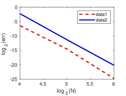
Refer to caption Refer to caption
(a) (b)
Figure 7: (a): Example 2; (b): Example 3.

Appendix

The Floquet-Bloch transform

The main tool used in this paper is the Floquet-Bloch transform. In this section, we will recall the definition and some basic properties of the Bloch transform in periodic domains in ℝd\mathbb{R}^{d} (for details see [Lec17]).

Suppose Ω⊂ℝd\Omega\subset\mathbb{R}^{d} is Λ\Lambda-periodic in x~\widetilde{x}-direction, i.e., for any x~⊤=(x~⊤,xd)∈Ω\widetilde{x}^{\top}=(\widetilde{x}^{\top},x_{d})\in\Omega, the translated point x+(Λ​j0)∈Ω,∀j∈ℤx+\left(\begin{smallmatrix}\Lambda j\\ 0\end{smallmatrix}\right)\in\Omega,\,\forall{j}\in\mathbb{Z}. Define one periodic cell by ΩΛ:=Ω∩[WΛ×ℝ]\Omega^{\Lambda}:=\Omega\cap\left[{W_{\hskip-1.0pt{\Lambda}}}\times\mathbb{R}\right]. For any φ∈C0∞​(Ω)\varphi\in C_{0}^{\infty}(\Omega), define the (partial) Bloch transform in Ω\Omega, i.e., 𝒥Ω\mathcal{J}_{\Omega}, of φ\varphi as

(𝒥Ωφ)(α,x)=CΛ∑j∈ℤd−1φ(x+(Λ​j0))e−iα⋅Λj,α∈ℝ,x∈ΩΛ\left(\mathcal{J}_{\Omega}\varphi\right)({\alpha},{x})=C_{\Lambda}\sum_{{j}\in\mathbb{Z}^{d-1}}\varphi\left({x}+\left(\begin{matrix}\Lambda{j}\\ 0\end{matrix}\right)\right)e^{-\mathrm{i}{\alpha}\cdot\Lambda{j}},\quad{\alpha}\in\mathbb{R},\,{x}\in\Omega^{\Lambda}

where CΛ=|Λ|2​πC_{\Lambda}=\sqrt{\frac{|\Lambda|}{2\pi}}. The Bloch transform is well-defined for any smooth function with compact support, and could be extended to more generalized Sobolev spaces.

Remark 26.

The periodic domain Ω\Omega is not required to be bounded in xdx_{d}-direction.

We can also define the weighted Sobolev space on the unbounded domain Ω\Omega by

Hrs​(Ω):={φ∈𝒟′​(Ω):(1+|x|2)r/2​φ​(x)∈Hs​(Ω)}.H_{r}^{s}(\Omega):=\left\{\varphi\in\mathcal{D}^{\prime}(\Omega):\,(1+|{x}|^{2})^{r/2}\varphi({x})\in H^{s}(\Omega)\right\}.

For any ℓ∈ℕ\ell\in\mathbb{N}, s∈ℝs\in\mathbb{R}, we can also define the following Hilbert space by

Hℓ​(WΛ∗,Hs​(ΩΛ)):={ψ∈𝒟′​(WΛ∗×ΩΛ):∑m=0ℓ∫WΛ∗‖∂αmψ⁡(α,⋅)‖​𝑑α<∞},H^{\ell}({W_{\hskip-1.0pt{\Lambda}^{\ast}}};H^{s}(\Omega^{\Lambda})):=\left\{\psi\in\mathcal{D}^{\prime}({W_{\hskip-1.0pt{\Lambda}^{\ast}}}\times\Omega^{\Lambda}):\,\sum_{m=0}^{\ell}\int_{W_{\hskip-1.0pt{\Lambda}^{\ast}}}\left\|\partial^{m}_{\alpha}\psi({\alpha},\cdot)\right\|\,\mathrm{d}\alpha\,<\infty\right\},

and extend the index ℓ∈ℕ\ell\in\mathbb{N} to any r∈ℝr\in\mathbb{R} by interpolation and duality arguments. The space H0r​(WΛ∗,Hαs​(ΩΛ))H_{0}^{r}({W_{\hskip-1.0pt{\Lambda}^{\ast}}};H_{\alpha}^{s}(\Omega^{\Lambda})) is the subspace of Hℓ​(WΛ∗,Hs​(ΩΛ))H^{\ell}({W_{\hskip-1.0pt{\Lambda}^{\ast}}};H^{s}(\Omega^{\Lambda})) such that all functions in the space is periodic with respect to α\alpha and quasi-periodic with respect to the second variable. The following properties for the dd-dimensional (partial) Bloch transform 𝒥Ω\mathcal{J}_{\Omega} is also proved in [Lec17].

Theorem 27.

The Bloch transform 𝒥Ω\mathcal{J}_{\Omega} extends to an isomorphism between Hrs​(Ω)H_{r}^{s}(\Omega) and H0r​(WΛ∗,Hαs​(ΩΛ))H_{0}^{r}({W_{\hskip-1.0pt{\Lambda}^{\ast}}};H_{\alpha}^{s}(\Omega^{\Lambda})) for any s,r∈ℝs,r\in\mathbb{R}. Its inverse has the form of

(𝒥Ω−1​ψ)​(x+(Λ​j0))=CΛ​∫WΛ∗ψ⁡(α,x)​ei​α⋅Λ​j​𝑑α,x1∈ΩΛ,j∈ℤ,(\mathcal{J}^{-1}_{\Omega}\psi)\left({x}+\left(\begin{matrix}\Lambda{j}\\ 0\end{matrix}\right)\right)=C_{\Lambda}\int_{W_{\hskip-1.0pt{\Lambda}^{\ast}}}\psi({\alpha},{x})e^{\mathrm{i}{\alpha}\cdot\Lambda{j}}\,\mathrm{d}\alpha\,,\quad x_{1}\in\Omega^{\Lambda},\,{j}\in\mathbb{Z},

and the adjoint operator 𝒥Ω∗\mathcal{J}^{*}_{\Omega} with respect to the scalar product in L2​(WΛ∗,L2​(ΩΛ))L^{2}({W_{\hskip-1.0pt{\Lambda}^{\ast}}};L^{2}(\Omega^{\Lambda})) equals to the inverse 𝒥Ω−1\mathcal{J}^{-1}_{\Omega}. Moreover, when r=s=0r=s=0, the Bloch transform 𝒥Ω\mathcal{J}_{\Omega} is an isometric isomorphism.

Another important property of the Bloch transform is the commutes with partial derivatives, see [Lec17]. If u∈Hrn​(Ω)u\in H_{r}^{n}(\Omega) for some n∈ℕn\in\mathbb{N}, then for any γ=(γ1,…,γd)∈ℕd{\gamma}=(\gamma_{1},\dots,\gamma_{d})\in\mathbb{N}^{d} with |γ|=≤N|\gamma|=\leq N,

∂xγ(𝒥Ω​u)​(α,x)=𝒥Ω​[∂γu]​(α,x).\partial^{\gamma}_{x}\left(\mathcal{J}_{\Omega}u\right)({\alpha},{x})=\mathcal{J}_{\Omega}[\partial^{\gamma}u]({\alpha},{x}).
Remark 28.

The definition of the partial Bloch transform could also be extended to other periodic domains, for example, periodic hyper-surfaces. If Γ\Gamma is a Λ\Lambda-periodic surface defined in ℝd\mathbb{R}^{d}, then we can define 𝒥Γ\mathcal{J}_{\Gamma} in the same way, and obtain similar properties. In this paper, we will denote the Bloch transform 𝒥X\mathcal{J}_{X} by the partial Bloch transform in the domain X⊂ℝdX\subset\mathbb{R}^{d}, which is periodic with respect to x~\widetilde{x}-direction.

Remark 29.

There is an alternative definition for the space H0r​(WΛ∗,Xα)H_{0}^{r}({W_{\hskip-1.0pt{\Lambda}^{\ast}}};X_{\alpha}), where XαX_{\alpha} is a family of Hilbert spaces that are α{\alpha}-quasi-periodic in x~\widetilde{x}. Let

φΛ∗(j)(α)=CΛe−iα⋅Λj,j∈ℤ\varphi_{\Lambda^{*}}^{({j})}({\alpha})=C_{\Lambda}e^{-\mathrm{i}{\alpha}\cdot\Lambda{j}},\,{j}\in\mathbb{Z}

be a complete orthonormal system in L2​(WΛ∗)L^{2}({W_{\hskip-1.0pt{\Lambda}^{\ast}}}), then any function ψ∈𝒟′​(WΛ∗×ΩΛ)\psi\in\mathcal{D}^{\prime}({W_{\hskip-1.0pt{\Lambda}^{\ast}}}\times\Omega^{\Lambda}) has a Fourier series

ψ(α,x)=CΛ∑ℓ∈ℤψ^Λ∗(ℓ,x)e−iα⋅Λℓ,\psi({\alpha},{x})=C_{\Lambda}\sum_{{\ell}\in\mathbb{Z}}\hat{\psi}_{\Lambda^{*}}({\ell},{x})e^{-\mathrm{i}{\alpha}\cdot\Lambda{\ell}},

where ψ^Λ∗​(ℓ,x)=<ψ⁡(⋅,x),φΛ∗(ℓ)>L2​(WΛ∗)\hat{\psi}_{\Lambda^{*}}({\ell},{x})=<\psi(\cdot,{x}),\varphi_{\Lambda^{*}}^{({\ell})}>_{L^{2}({W_{\hskip-1.0pt{\Lambda}^{\ast}}})}. Then the squared norm of any ψ∈H0r​(WΛ∗,Xα)\psi\in H_{0}^{r}({W_{\hskip-1.0pt{\Lambda}^{\ast}}};X_{\alpha}) equals to

‖ψ‖H0r​(WΛ∗,Xα)2=∑ℓ∈ℤ(1+|ℓ|2)r​‖ψ^Λ∗​(ℓ,⋅)‖Xα2.\|\psi\|^{2}_{H_{0}^{r}({W_{\hskip-1.0pt{\Lambda}^{\ast}}};X_{\alpha})}=\sum_{{\ell}\in\mathbb{Z}}(1+|{\ell}|^{2})^{r}\left\|\hat{\psi}_{\Lambda^{*}}({\ell},\cdot)\right\|^{2}_{X_{\alpha}}.

8.1 Cutoff functions

We look for a smooth cutoff functions gg in the interval [a,b][a,b] such that

g(a)=0,g(b)=1,g(j)(a)=g(j)(b)=0 for any j=1,2,…,n,g(a)=0,\,g(b)=1,\,g^{(j)}(a)=g^{(j)}(b)=0\text{ for any }j=1,2,\dots,n, (114)

where n∈ℕ+n\in\mathbb{N}^{+} is a positive integer. We can define the function by

g⁡(t)=c​∫at(τ−a)n+1​(b−τ)n+1​𝑑τ,g(t)=c\int_{a}^{t}(\tau-a)^{n+1}(b-\tau)^{n+1}\,\mathrm{d}\tau\,, (115)

where the constant cc is defined by

c=(∫ab(τ−a)n+1​(b−τ)n+1​𝑑τ)−1.c=\left(\int_{a}^{b}(\tau-a)^{n+1}(b-\tau)^{n+1}\,\mathrm{d}\tau\,\right)^{-1}. (116)

If the cutoff function satisfies

g(a)=0,g(b)=1,g(j)(a)=g(j)(b)=0 for any j=1,2,…,∞,g(a)=0,\,g(b)=1,\,g^{(j)}(a)=g^{(j)}(b)=0\text{ for any }j=1,2,\dots,\infty, (117)

we can define

g⁡(t)=c​∫atexp⁡[−1((a+b)/2)2−(τ−(b−a)/2)2]​𝑑τ,g(t)=c\int_{a}^{t}\exp\left[-\frac{1}{((a+b)/2)^{2}-(\tau-(b-a)/2)^{2}}\right]\,\mathrm{d}\tau\,, (118)

where

c=(∫abexp⁡[−1((a+b)/2)2−(τ−(b−a)/2)2]​𝑑τ)−1.c=\left(\int_{a}^{b}\exp\left[-\frac{1}{((a+b)/2)^{2}-(\tau-(b-a)/2)^{2}}\right]\,\mathrm{d}\tau\,\right)^{-1}. (119)

References

  • [CE10] S. N. Chandler-Wilde and J. Elschner. Variational approach in weighted Sobolev spaces to scattering by unbounded rough surfaces. SIAM. J. Math. Anal., 42:2554–2580, 2010.
  • [CM05] S. N. Chandler-Wilde and P. Monk. Existence, uniqueness, and variational methods for scattering by unbounded rough surfaces. SIAM. J. Math. Anal., 37:598–618, 2005.
  • [Coa12] J. Coatléven. Helmholtz equation in periodic media with a line defect. J. Comp. Phys., 231:1675–1704, 2012.
  • [CWHP06] S. N. Chandler-Wilde, E. Heinemeyer, and R. Potthast. A well-posed integral equation formulation for 3d rough surface scattering. Proceedings of the Royal Society of London, Series A 462:3683–3705, 2006.
  • [CWRZ99] S.N. Chandler-Wilde, C.R. Ross, and B. Zhang. Scattering by infinite one-dimensional rough surfaces. Proceedings of the Royal Society A, 455:3767–3787, 1999.
  • [CWZ96] S. N. Chandler-Wilde and B. Zhang. On the solvability of a class of second kind integral equations on unbounded domains. Journal of Mathematical Analysis and Applications, 241:482–502, 1996.
  • [HLP88] G. H. Hardy, J. E. Littlewood, and G. Pólya. Inequalities. Cambridge Mathematical Library. Cambridge University Press, 2nd edition, 1988.
  • [HN16] H. Haddar and T. P. Nguyen. A volume integral method for solving scattering problems from locally perturbed infinite periodic layers. Appl. Anal., 96(1):130–158, 2016.
  • [Lec17] A. Lechleiter. The Floquet-Bloch transform and scattering from locally perturbed periodic surfaces. J. Math. Anal. Appl., 446(1):605–627, 2017.
  • [LN15] A. Lechleiter and D.-L. Nguyen. Scattering of Herglotz waves from periodic structures and mapping properties of the Bloch transform. Proc. Roy. Soc. Edinburgh Sect. A, 231:1283–1311, 2015.
  • [LZ17a] A. Lechleiter and R. Zhang. A convergent numerical scheme for scattering of aperiodic waves from periodic surfaces based on the Floquet-Bloch transform. SIAM J. Numer. Anal, 55(2):713–736, 2017.
  • [LZ17b] A. Lechleiter and R. Zhang. A Floquet-Bloch transform based numerical method for scattering from locally perturbed periodic surfaces. SIAM J. Sci. Comput., 39(5):B819–B839, 2017.
  • [LZ17c] A. Lechleiter and R. Zhang. Non-periodic acoustic and electromagnetic scattering from periodic structures in 3d. Comput. Math. Appl., 74(11):2723–2738, 2017.
  • [MACK00] A. Meier, T. Arens, S. N. Chandler-Wilde, and A. Kirsch. A Nyström method for a class of integral equations on the real line with applications to scattering by diffraction gratings and rough surfaces. J. Int. Equ. Appl., 12:281–321, 2000.
  • [MC01] A. Meier and S. N. Chandler-Wilde. On the stability and convergence of the finite section method for integral equation formulations of rough surface scattering. Math. Methods. Appl. Sci., 24:209–232, 2001.
  • [SS07] S. Sauter and C. Schwab. Boundary Element Methods. Springer, Berlin-New York, 2007.
  • [ZCW03] B. Zhang and S. N. Chandler-Wilde. Integral equation methods for scattering by infinite rough surfaces. Math. Meth. Appl. Sci., 26:463–488, 2003.
  • [Zha18a] R. Zhang. A bloch transform based numerical method for the rough surface scattering problems. https://arxiv.org/pdf/1805.11484.pdf, 2018.
  • [Zha18b] R. Zhang. A high order numerical method for scattering from locally perturbed periodic surfaces. SIAM J. Sci. Comput., 40(4):A2286–A2314, 2018.
  • [Zha18c] R. Zhang. Scattering problems from multi-layers with different periodicities. https://arxiv.org/pdf/1806.05063.pdf, 2018.
  • [Zha18d] R. Zhang. Scattering problems from slightly perturbed periodic surfaces: Part i. 2018.